Fuzzy Logic Classification of Imaging Laser Desorption Fourier Transform Mass Spectrometry Data

Abstract

A fuzzy logic based classification engine has been developed for classifying mass spectra obtained with an imaging internal source Fourier transform mass spectrometer (I²LD-FTMS). Traditionally, an operator uses the relative abundance of ions with specific mass-to-charge (m/z) ratios to categorize spectra. An operator does this by comparing the spectrum of m/z versus abundance of an unknown sample against a library of spectra from known samples. Automated positioning and acquisition allow I²LD-FTMS to acquire data from very large grids, this would require classification of up to 3600 spectrum per hour to keep pace with the acquisition. The tedious job of classifying numerous spectra generated in an I²LD-FTMS imaging application can be replaced by a fuzzy rule base if the cues an operator uses can be encapsulated. We present the translation of linguistic rules to a fuzzy classifier for mineral phases in basalt. This paper also describes a method for gathering statistics on ions, which are not currently used in the rule base, but which may be candidates for making the rule base more accurate and complete or to form new rule bases based on data obtained from known samples. A spatial method for classifying spectra with low membership values, based on neighboring sample classifications, is also presented.

1 Introduction

The Idaho National Laboratory (INL) has produced an imaging internal laser desorption Fourier transform mass spectrometer (I²LD-FTMS) that provides the chemical imaging for the laser-based optical and chemical imager (LOCI). The I²LD-FTMS couples a unique laser-scanning device [Scott and Tremblay (2002)] with the mass analyzer operating commercial Finnigan FT/MS software (Bremen, Germany). It is capable of acquiring mass spectral data from numerous locations on a sample while tracking the x,y-positions. The positioning of the laser-scanning device and acquisition of mass spectral data has been fully automated [McJunkin et al. (2002)]. The I²LD-FTMS generates a plethora of data as up to 3600 files per hour can be acquired. Manual analysis of this data would be a daunting task; therefore, we have developed a data classifying agent to analyze the data and produce a classification map of the sample.

Automation of mass spectra interpretation has been reported for peptides and proteins [Horn et al. (2000)], pharmaceuticals [Korfmacher et al. (1999)], and glycerolipids [Kurvinen et al. (2002)]. Some researchers have applied all data points from a mass spectrum as inputs to a neural network with an output for each classification [Klawun and Wilkins (1996)]. This method works well for complex spectra where the number of inputs cannot be reduced. More complicated solution surfaces lead to more computation requirements and less transparency in the decision process. Training methods for the neural networks have been applied [Klawun and Wilkins (1996), Ingram et al. (1999)]. Others have defined branching decision trees to implement expert systems [Georgakopoulos et al. (1998)]. Still others have defined typical relative abundance of a set of key ions as a vector for each class [Ingram et al. (1999)]. They then chose the class with the minimum Euclidean distance to a given sample spectrum.

Manual basalt mineral phase classification using mass spectra is accomplished by analyzing the relative peak abundances versus mass-to-charge (m/z) ratios. Traditionally, an analyst builds a repertoire of spectral characteristics by inspecting spectra from known homogeneous mineral types. Assignment of spectra from unknown or heterogeneous samples is then accomplished by comparison with the reference spectra of the known mineral types. In the case of basalt phases, it was noticed that the relative magnitude of specific key peaks to each other are the primary cues for classifying the data. This handful of peaks corresponds to the ions whose relative abundance determines the appropriate mineral classification.

To classify basalt, Ingram et al. [Ingram et al. (1999)] used a neural network based vector quantization to group spectra and then assign a classification to each group, providing a way to find classification with a priori knowledge of only the significant ions. However, the Euclidean distance used in this method can result in incorrect assignment of class due to the arbitrary assignment of the average abundance of an ion that is unimportant to a particular classification. An abundance for such an ion could contribute to the Euclidean distance to the center of an incorrect class being shorter than to the center of the appropriate classification. Our method is similar in selecting a small group of ions as inputs to classify the spectra. However, a fuzzy logic [Zadeh (1965), Lee (1990a), Lee (1990b)] membership function approach is used in place of a Euclidean distance, which allows full membership to be assigned over a range of relative abundance rather than specifying a single exact value and also provides for exclusion of ions from specific classifications (i.e. a logical don’t care).

Section 2 describes the inference engine developed to classify mass spectra and is illustrated for mineral types found in basalt samples. The rules for the inference process were derived from analyzing the process that a human analyst used in classifying the mass spectra. The inference process was distilled to a concise set of rules that could be implemented with fuzzy logic. Subsequently, a method for building statistics, which assists in determining appropriate rules, was developed. This method, which also allows the identification of other key ions or subclassifications and may be a basis for future work on statistical classification methods, is described in Section 3. In Section 4, a useful method for classifying a mass spectrum, which is classified as unknown, based on the membership values in mineral sets and the classification of the location’s neighbors is discussed. Finally, results and conclusions are presented.Comparison of this fuzzy method to principle component analysis and K-means clustering has been reported in Yan, et.al. [Yan et al. (2006)].

2 Classification of Spectra with Fuzzy Thresholds

A mineral phase in a basalt sample can be identified by its chemical composition [Deer et al. (1992)]. In particular, the relative abundance of particular ions give the signature for a specific mineral type. The laser desorption process lifts both ions of elements and molecules from the surface of the rock sample. These ions are trapped in the Fourier transform mass spectrometer cell where they are excited with a chirped radio frequency field driven across a band from $50hz\rightarrow 4Mhz$ at a sweep rate of $3500hz/\mu S$. A Fourier transform (FT) is applied to the digitized signal received from the sense plates, which are orthogonal to the excite plates. The frequency scale of the FT has a one-to-one correspondence with the m/z of the ion whose excitation induced the frequency in the sense plates.

A natural fit for fuzzy logic was found when analytical chemist described the decision for classification as: “The basalt phase Augite has significant abundance of iron, large abundance of calcium and little or no titanium.” The linguistic description, void of explicit thresholds, provided a direct path to fuzzy logic expression of classification rules.

Another reason for using fuzzy membership functions in FTMS mineral identification is the magnitude of a particular peak is proportional to the abundance of ions with the corresponding m/z. However, for at least a couple of reasons, precise abundance results are not expected. For one, the efficiency of the laser desorption/ionization process varies for different elements and is also influenced by the matrix that entrains the element; therefore, the ion abundance is not strictly proportional to the elemental percent composition expected for a given mineral. Secondly, the finite spot size of the laser can desorb multiple mineral types at a single sample location. A fuzzy logic based decision can interpolate, with some success, between mineral types when ions from various mineral types are “blended”.

2.1 Fuzzification

Mass-to-charge peaks that affect the expert classification are converted to a fuzzy logic level based on their relative abundance. The truth level for a particular ion in a specific classification can be Boolean by setting a threshold: when the abundance is above the appropriate side of the threshold, the truth level is high. It is convenient to allow for a gray area with a piece-wise linear function mapping the abundance into a $[0,1]$ range, so that an abundance just outside the threshold can have a graduated approach in its affect on the classification.

A given mineral type will require that several ions be present or absent in a range of relative abundances. The requirement for a specific ion is encoded in a fuzzy membership function $\mu_{\gamma,\chi}(A)$ where $\gamma$ is the mineral classification, $\chi$ is a specific ion denoted as a chemical symbol or the m/z of the ion, and $A$ is the mass spectrum of the sample being classified. The spectrum, $A$, can be represented as the relative abundance as a function of m/z, $a(\phi)$, where $\phi$ is the m/z. The first step in finding $\mu_{\gamma,\chi}(A)$ is locating the maximum abundance, $p$, within the error bound, $\epsilon$, of $\chi$:

$$p(A,\chi)=\max_{\phi=\chi-\epsilon}^{\chi+\epsilon}(a(\phi)).$$ (1)

The error bound is required because of uncertainty due not only to drift in magnetic field strength between calibrations but to an electric space-charge effect depending on the number of ions desorbed [Marshall and Verdun (1990)] (pages 244-245).

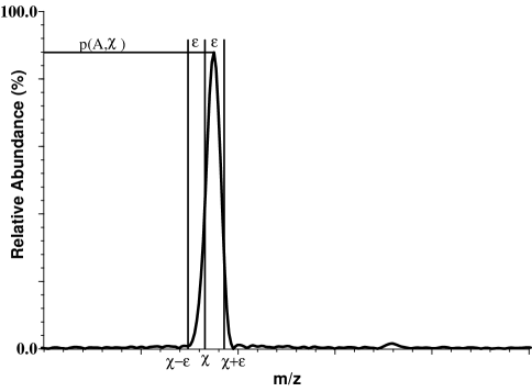
Figure 1: Illustration of maximum abundance within $\epsilon$ of $\chi$.

The membership value then becomes a function mapping $p$ onto a fuzzy logical level, $[0,1]$. The linguistic expression for whether an ion’s abundance is appropriate for a particular mineral composition can take a form similar to: “the relative abundance of iron should be small” or “the relative abundance of calcium (Ca) should be high.” The level at which the logic level is $100\%$ true or false is a judgement call, which can better be performed by allowing interpolation. Experts could conceivably compromise on levels of abundance that constitute an absolute true or false and allow a function to interpolate between those levels. For lack of apparent need for a more complex interpolation, we chose to implement a piece-wise linear function. In general we could have medium relative abundance functions; but, in practice, we have only found need to define functions for relative high or low abundances. The low (not) abundance function can be formed as the negative of a high abundance function. So, $\mu$ takes one of the two forms, shown in Fig. 2:

$$\mu_{\gamma,\chi}(p)=\left\{\begin{array}[]{ll}0&p<l\\ \frac{p-l}{h-l}&l\leq p<h\\ 1&p\geq h\end{array}\right.$$ (2)

for required high abundance, or for low abundance

$$\mu_{\gamma,\sim\chi}(p) = 1-\mu_{\gamma,\chi}(p)$$ (6)

$$= \left\{\begin{array}[]{ll}1&p<l\\ \frac{h-p}{h-l}&l\leq p<h\\ 0&p\geq h\end{array}\right.,$$

where $l$ is low hard logic threshold and $h$ is the high logic threshold, $l<h$, and the symbol ‘$\sim$’ indicates the negation (i.e. NOT $\chi$). The primary method for choosing $l$ and $h$ has an expert operator look at many spectra taken from various locations on a homogeneous “known.” From these observations thresholds can be set and the size of the “gray” area chosen.

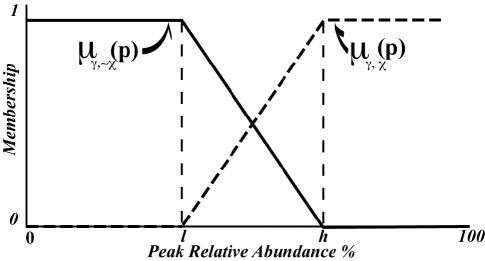
Figure 2: Examples of membership function for high and low abundance requirements.

2.2 Inference Rules

Inference rules are based on logical expressions of requirements. The fuzzy membership functions determine the truth value of each term in the expression. Logical operations are defined using the logic levels from the fuzzy membership values of an ion with respect to the mineral class. The “and” ($\wedge$) function is implemented with the product operation ($A\wedge B\rightarrow\mu_{A}\mu_{B}$), the “or” ($\vee$) function with the equivalent ($A\vee B\rightarrow\mu_{A}+\mu_{B}-\mu_{A}\mu_{B}$), and “not” ($\sim$) as negation, $1-\mu$. As an example, our rule for augite (AGT) has requirements on the ions of iron (Fe), titanium (Ti) and Ca. The expression for membership in the class AGT is the product of the result of the membership functions, $\mu_{{AGT},Fe}$, $\mu_{{AGT},\sim Ti}$, and $\mu_{{AGT},Ca}$ and can be written compactly as:

$$\mu_{AGT}(A)=\bigwedge_{\chi\in}^{\{Fe,\sim Ti,Ca\}}\mu_{{AGT},\chi}(A).$$ (7)

The benefit of using the product operation over minimums and maximums is the additive affect in the “or” terms. In particluar, ilmenite is defined as having one or more of the metals, Fe, magnesium (Mg), or manganese (Mn), above a certain accumulative abundance. This allows the membership function to be constructed such that appropriate combination of the metals will give a sufficiently high membership value. The product implementation for “and” terms also discounts membership of multiple terms below full membership, providing a more conservative approach (e.g. two terms of membership value $0.9$ “and”-ed together discounts the resulting membership value to $0.81$ instead of the minimum value $0.9$).

2.3 Hard Classification

Although leaving the result of the classification as the value of the fuzzy membership in each the mineral classes is useful in some applications, our current application requires discrete classifications. Defuzzification is accomplished by finding the mineral class with the maximum membership value. A threshold, $\nu$, is set at a minimum required membership. If the spectra does not have a maximum membership in one of the classes greater than $\nu$ then it is classified as unknown, UNK. The hard classification, $\Gamma$ is:

$$\Gamma(A)=\left\{\begin{array}[]{ll}(\gamma|\mu_{\gamma}=\displaystyle\max_{\chi}\mu_{\chi})&\mbox{for}\displaystyle\max_{\chi}\mu_{\chi}\geq\nu\\ \mbox{UNK}&\mbox{for}\displaystyle\max_{\chi}\mu_{\chi}<\nu\end{array}\right.$$ (8)

As a side note, the membership value in the set of UNK can be defined as the negation of the maximum membership value: $\mu_{\mbox{UNK}}=1-\max_{\chi}\mu_{\chi}$.

Unknown spectra are left for the instrument operator to classify or remain as ‘unknown.’ An unknown spectra may occur when the desorption laser spot covers more than one class of mineral or there is a problem with the desorption process or acquired signal. An automated method for assigning a value based on the membership values and the neighboring spots in the sample is presented in Section 4.

One item of note, some basalt samples from the INL site have the characteristic of an unusually high potassium abundance not noted in the mineral literature [Deer et al. (1992)]. This has been reported in other mass spectrometry literature for analysis of INL basalt [Ingram et al. (1999)]. To adjust for the high potassium abundance, spectra used by the inference engine are preprocessed to re-scale based on the highest peak excluding potassium. The software implementing the system allows particular ions to be rescaled in this way when required.

3 Ensemble Statistics for Generating and Refining Rulebases

In this section, a spectra statistical method is presented for determining or refining rules given a set of data. The method acts on a set of spectra that have been classified as the same type of mineral by the rule base, are from a known homogeneous sample, or from a diverse ensemble. Several statistics are accumulated across all sample data about the peaks in the spectra: sum, sum of squares, minimum and maximum of abundances, and count of non-zero abundances. The size of bins used to sort peaks into is determined by the mass accuracy of the FTMS.

Given a set of spectra, $F$, which have the same classification, composed of $\{A_{1},...,A_{n}\}$, we want to look for similarities in the mass spectra. A data base containing m/z, number of spectra with a peak of the m/z, the total relative abundance, and the sum of the square of the abundance is generated. A list of local maxima or “peak list” of a spectrum can be used to represent $A$, $\bar{a}=\{(\phi[1],\bar{a}[1]),...,(\phi[n],\bar{a}[n])\}$, where $n$ is the number of local maxima in $a(\phi)$ and the list is sorted on $\phi$. If two or more peaks have $\phi$ within $\epsilon$ of each other, we form a consolidated list ($\hat{a}$) of only the maximum abundance of these peaks.

A statistical data base element, $S[i]$, is created for each bin of $\phi$ within $\epsilon$ of each other. The fields of the data base will be noted with $S[i].field$. The first element is the m/z of the bin, $S[i].\phi$. We chose to calculate this as the mean of the $\phi$ in spectra with a peak in the $i^{\mbox{th}}$ bin, though there are many ways (weight average, $\phi$ of maximum abundance, etc.) which could be used. The total count of spectra containing a non-zero abundance peak within $\epsilon$ of $\phi$ is tabulated in $S[i].c$. The sum, sum of squares, max, and min of the abundance for the peaks with spectra fitting the same requirement are accumulated in $S[i].a_{tot}$, $S[i].a_{tot}^{2}$, $S[i].a_{max}$, and $S[i].a_{min}$, respectively. These are typical statistics for determining mean, standard deviation, and count for a given m/z peak.

Additional key ions that positively discriminate one class versus the remainder of the classifications can be determined using the statistics of spectra from that class versus the statistics of the ensemble of the diverse spectra from the other classes. By selecting the $S[i]$ with $S[i].c$ equal to the total count of spectra classified in the class, candidates for unique positive cues for the class are obtained. When the mean of the abundances $S[i].a_{tot}/S[i].c$ is compared to the mean of the abundances for data in all classifications, a ratio significantly larger than $1$ is motivation to investigate the peak as a possible key ion. Alternatively, a result of a small value for $S[i].a_{tot}$ divided by the total count of spectra in the classification, including the zero abundance spectra in the average, can be compared to the mean of the whole of the data. If the ratio of the class mean to the ensemble the peak may also provide a distinguishing characteristic of a low abundance compared to the entire set. An example is shown in Section 5.

This set of statistics can be utilized to locate distinct peaks to this classification, if a particular $S[i]$ is unique to the classification $F$. It can also be used to identify sub-classifications or contaminants, if a subset of $F$ all contain unique peaks compared to the rest of $F$. A bifurcation of the classification into subclassifications may be indicated by a count of abundances less than the total count of the spectra in the set. A further extension of this concept would be to look for separation(s) in the abundances for a given m/z into two or more clusters.

Finally if the spectra are from a homogeneous sample of material, which does not have a set of inference rules, a rule base can be derived from these statistics using key peaks. While not currently automated, the tools outlined in this section provide methods that are used to create and refine rules based on accumulated statistics.

4 Spatially Based Classification of Indeterminate Samples

Occasionally, a spectrum will be a combination of minerals types or be overwhelmed by an anomalous ion, such as potassium, or of low magnitude because of degraded vacuum. For cases where there are sporadic “unknown” spots, a method for filling in the unknowns based on the surrounding spots is desirable. Such a method is described in this section.

The membership value of a particular spot for a class, $\gamma$, is denoted by, $\mu_{\gamma}[i]$, where $i$ is an index for the spot. The index, $i$, maps to a Cartesian coordinate of the spot. Typical spot patterns are either rectangular grids or hexagonal (closest pack) grids, see Fig. 3 . For this method we identify the neighbors of the unknown spot and modify the membership value of the unknown spot based on the the membership values of the surrounding spots:

$${\bar{\mu}}_{\gamma}[i]=\mu_{\gamma}[i]+\displaystyle\sum_{j}^{\mbox{neighbors}}\frac{\mu_{\gamma}[j]}{N},$$ (9)

where $N$ is the number of neighboring spots. The membership value of spot $i$ is added to the average of the spots near it. The hard classification is made by finding the maximum membership value:

$$\Gamma[i]=\left\{\begin{array}[]{ll}(\gamma|\mu_{\gamma}[i]=\displaystyle\max_{\chi}\mu_{\chi}[i])&\mbox{for}\displaystyle\max_{\chi}\mu_{\chi}[i]\geq\nu\\ (\gamma|{\bar{\mu}}_{\gamma}[i]=\displaystyle\max_{\chi}{\bar{\mu}}_{\chi}[i])&\mbox{for}\displaystyle\max_{\chi}{\mu}_{\chi}[i]<\nu\par\end{array}\right..$$ (10)

Fig. 3 shows the neighboring spots which would be selected. If the spot is at an edge or corner of the data set $N$ would be reduced appropriately for missing spots.

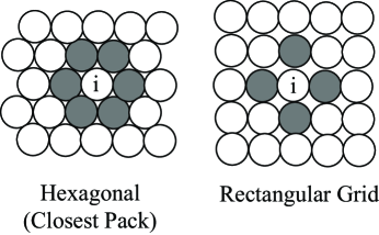
Figure 3: Neighbors used for classifying unknown are shown as gray for the two typical spot patterns.

5 Results and Discussion

The methods described in the previous sections have been applied to basalt samples. This section will describe the resulting rule base and the steps taken to arrive at the current solution. Finally, a set of results from a sample of basalt is given with discussion on the result.

The rules were developed in a progression: (1) FTMS operator observed spectra from homogeneous samples of the expected mineral phases; (2) additions and modifications to the rules where made based on survey of mineral reference literature [Deer et al. (1992)]; (3) the tool for grouping statistics was developed and used to identify additional ions and shape membership functions; and (4) a method for making a good guess at spots that were unknown to the inference engine was developed for data presentation requiring a complete map.

The use of fuzzy logic was prompted by the realization that the FTMS operator used phrases such as, “Ilmenite has a high abundance of Ti and Fe compared to other mineral phases.” Based on tabulated chemical composition data [Deer et al. (1992)] from various samples of the mineral phases of interest from around the world, the rules were refined. For example, the reference literature made clear that plagioclase should contain a significant abundance of Al. Aluminum was initially overlooked because its relative abundance is lower than that of the primary cue of Ca from the plagioclase samples. In fact, Ca is a don’t care ion because some varieties of plagioclase do not contain Ca. This emphasizes that a human can be fooled without the appropriate visualization tool.

Although the appropriate use of compiled reference data should not be undervalued, the tool for accumulating statistics also showed that Al was an important indicator in plagioclase. Fig. 4 displays the ratio of the average abundance of ions occurring in a homogeneous sample of plagioclase to the average abundance of the ions in an ensemble of all mineral phase samples tested. Only the ions which were present in all of the plagioclase spectra are shown. The only ions whose average abundance in plagioclase is significantly above the ensemble average are Al and Ca. Al is an important constituent that was initially overlooked because the relative magnitude of the abundance was small compared to the other ions. If one has confidence in the known samples, the visualization tool can be used to find the unique cues between types that will allow for classification rules to be generated.

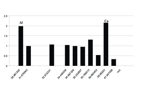
Figure 4: Average abundance of peaks in plagioclase samples spectra plagioclase relative to average abundance an ensemble of spectra from various “knowns.” Only ions which were contained in all plagioclase samples are displayed in the histogram. Note only Al and Ca are significantly above the average of the ensemble and Ca is known to be absent in some plagioclase from other geological areas.

Finally, there are circumstances where the spectrum from a spot are not identifiable. For example, in the case of degraded vacuum with the FTMS, the signals are too weak to generate a spectra above the noise level threshold set for the system. A more typical example is when a spot is too large to desorb only one mineral type. For applications where we need to classify all spots regardless of confidence in the data, we argue that proximity of like minerals should influence the decision. To this end, the method in Section 4 was created.

The result of this process has development of the rules listed in Table 1 for classification of the four basic types of minerals found in basalt in the Snake River vadose zone. Those types include: olivine (OLV), augite (AGT), ilmenite (ILM), and plagioclase (PLG).

Table 1: Definition of inference engine for classification of mineral types in basalt.

Ilmenite (ILM)
$\mu_{\mbox{ILM}}=\displaystyle\bigwedge_{\chi\in}^{\{Fe,Ti,\sim Al\}}\mu_{\mbox{ILM},\chi}$
$\chi$ (Chem/mz)	$l$	$h$
$\sim Al/26.982$	$0.5$	$15$
$Ti/47.95$	$1$	$17$
$Fe/55.954$	$1$	$40$
Augite (AGT)
$\mu_{\mbox{AGT}}=\displaystyle\bigwedge_{\chi\in}^{\{Fe,\sim Ti,Ca\}}\mu_{\mbox{AGT},\chi}$
$\chi$ (Chem/mz)	$l$	$h$
$Ca/39.95$	$50$	$80$
$\sim Ti/47.95$	$1$	$17$
$Fe/55.954$	$1$	$30$
Plagioclase (PLG)
$\mu_{\mbox{PLG}}=\displaystyle\bigwedge_{\chi\in}^{\{Al,\sim Fe,\sim Ti\}}\mu_{\mbox{PLG},\chi}$
$\chi$ (Chem/mz)	$l$	$h$
$Al/26.982$	$0.5$	$15$
$\sim Ti/47.95$	$1$	$17$
$\sim Fe/55.954$	$10$	$40$
Olivine (OLV)
$\mu_{\mbox{OLV}}=$	$(\mu_{\mbox{OLV},Mg}\vee\mu_{\mbox{OLV},Mn}\vee\mu_{\mbox{OLV},Fe})$
	$\wedge\sim\mu_{\mbox{OLV},Ti}\wedge\sim\mu_{\mbox{OLV},Al}$
$\chi$ (Chem/mz)	$l$	$h$
$Mg/24.312$	1	50
$\sim Al/26.982$	$0.5$	$15$
$\sim Ti/47.95$	$1$	$17$
$Mn/54.938$	$10$	$40$
$Fe/55.954$	$10$	$40$

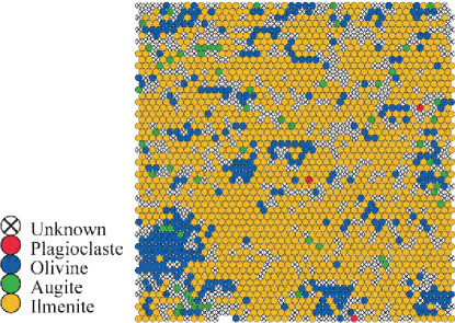
Figure 5: Classification mapping of an area of a sample of basalt from the Snake River vadose zone. Four graphs, b)-e), show the membership value of the spots. This is a hard classification map without applying the technique in Section 4. Spots are spaced $30\mu m$ apart (center to center).

The map in Fig. 5 shows an image of a section of basalt from the INL site. Without applying the technique described in Section 4 and choosing $\nu=0.5$, the hard classification in Fig. 5 shows some unknown spots. Membership values in individual classification is shown in Fig. 6. Fig. 7. shows the result of using the neighboring spots to help classify the unknowns. It is possible that the spot size used in this example was too large to be focused on individual mineral phases for some of the spots, where the two adjacent phases have a pair of mutually exclusive ion requirements and both are assigned a low membership value, resulting in the unknown classification. For example, the spot could contain both ilmenite and plagioclase, so the appearance of significant amounts of Ti and Al eliminate both classes from consideration. In another example, a high membership value of two classes indicates an overlap even though the hard classification chooses the highest level. Both of these cases would be resolved, except on the exact borders of mineral phases, by reducing the laser desorption spot size. However, there may always be cases where some of the mineral microcrystals are too small for the smallest laser spot size used. Therefore, using the nearest neighbor protocol will allow the unknown spots to be assigned and the membership value can be referenced to find a overlap of classes to a spot. Alternatively the hard classification can be adjusted to assign unknown to the case where we have multiple high membership value.

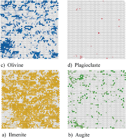
Figure 6: Fuzzy membership value for each classification.

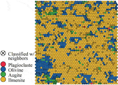
Figure 7: Classification mapping after applying near neighbors to unknowns.

6 Conclusion and Future Directions

The fuzzy logic inference engine described in the paper has been shown to accurately classify minerals in basalt. The automated classification system the inference engine provides is required to process the large amounts of data produced by an imaging FTMS. It has some advantages over other schemes used in the field. Specifically, it is simpler and more transparent in operation than neural networks. Also, the inference engine has flexibility to implement don’t care statements for the presence of specified ions, because Another important feature is the ability to leave a don’t care ion out of the logic expression, which avoids the problem of using an Euclidean measure. The output of the fuzzy logic inference engine provides a confidence level that can allow a human operator’s attention be drawn to the questionable and possibly interesting data in a large image. Additionally, a statistical visualization tool has been created to assist in developing rules for classification. Finally, a method for assigning indeterminate spots was described and illustrated.

In the future, rule bases for different types of materials will be created. For example, classification of soils will also be examined with the system. Additionally, the presence and type of microorganisms residing on basalt will be incorporated into the rule base. The input to the rule base will also be extended to the optical spectra that are also acquired as part of the overall LOCI instrument. Additionally automation of the methods discussed for generating and refining of rule bases will be investigated.

7 Acknowledgements

We thank Paul L. Tremblay for editorial suggestions to this paper and for being instrumental in the design and construction of the imaging FTMS. This work was supported by the U.S. Department of Energy under DOE/NE Idaho Operations Office Contract DE-AC07-05ID14517.

8 List of Symbols

For the readers convenience, the following is a list of symbols and variable notations used throughout the paper.

$A$	$\bullet$	FTMS spectrum to be analyzed.
$\gamma$	$\bullet$	variable to represent a mineral classification
$\chi$	$\bullet$	variable for a particular ion, indicated by either the chemical symbol or the m/z of the ion.
$\phi$	$\bullet$	variable for m/z.
$a(\phi)$	$\bullet$	a function representing $A$ as the abundance as a function of m/z.
$\hat{a}$	$\bullet$	peak list representation of $A$ as ordered pairs $(\bar{a},\phi)$ of local maxima of $a(\phi)$.
$p(A,\chi)$	$\bullet$	peak abundance of spectrum $A$ within $\epsilon$ of m/z for ion $\chi$
$\epsilon$	$\bullet$	error bound around the m/z for an ion $\chi$ for finding peak abundance.
$\mu_{\gamma}(A)$	$\bullet$	membership value for $A$ in the mineral classification, $\gamma$.
$\mu_{\gamma,\chi}(A)$	$\bullet$	membership value for a FTMS spectrum $A$ for mineral classification $\gamma$ and ion $\chi$.
$\mu_{\gamma,\chi}(p)$	$\bullet$	membership value requiring a high abundance for the peak, $p$, for mineral classification $\gamma$ and ion $\chi$.
$\mu_{\gamma,\sim\chi}(p)$	$\bullet$	membership value requiring a low abundance for the peak, $p$, for mineral classification $\gamma$ and ion $\chi$ (equivalent to $1-\mu_{\gamma,\chi}(p)$).
$\mu_{\gamma}[i]$	$\bullet$	membership value of the $i^{th}$ desorption spot in the class, $\gamma$.
${\bar{\mu}}_{\gamma}[i]$	$\bullet$	membership value of the $i^{th}$ desorption spot in the class, $\gamma$, biased by its neighboring spots.
$\wedge$	$\bullet$	fuzzy logic “and” operator defined for this paper as the product of the two operands, $\mu_{A}\mu_{B}$.
$\vee$	$\bullet$	fuzzy logic “or” operator defined as the logical inverse of the product of the two operands, $\mu_{A}+\mu_{B}-\mu_{A}\mu_{B}$.

$\nu$	$\bullet$	threshold value setting the minimum membership value to determine the “hard” classification
$\Gamma(A)$	$\bullet$	Defuzzification function returning the “hard” classification or “unknown.”
$\Gamma[i]$	$\bullet$	Defuzzification function returning the “hard” classification for the $i^{th}$ desorption spot.
$S[i].\phi$	$\bullet$	Center m/z of the $i^{\mbox{th}}$ bin
$S[i].a_{tot}$	$\bullet$	Total abundance from all spectra—used to compute the mean
$S[i].a_{tot}^{2}$	$\bullet$	Sum of the square of abundance—for calculation of standard deviation
$S[i].a_{max}$	$\bullet$	Maximum abundance for $i^{\mbox{th}}$ bin
$S[i].a_{min}$	$\bullet$	Minimum abundance
$S[i].c$	$\bullet$	Count of spectra with a non-zero peak in the $i^{\mbox{th}}$ bin.

References

- Deer et al. (1992) Deer, W., R. Howie, and J. Zussman: 1992, An Introduction to the Rock-Forming Minerals, Second Edition. Essex, England: Prentice Hall.
- Georgakopoulos et al. (1998) Georgakopoulos, C. G., M. Statheropoulos, and G. Montaudo: 1998, ‘An expert system for the interpretation of pyrolysis mass spectra of condensation polymers’. Analytica Chmica Acta 359, 213–225.
- Horn et al. (2000) Horn, D. M., R. A. Zubarev, and F. W. McLafferty: 2000, ‘Automated de novo sequencing of proteins by tandem high-resolution mass spectrometry’. In: Proceedings of the National Academy of Sciences of the United States of America, Vol. 97.
- Ingram et al. (1999) Ingram, J. C., G. S. Groenewold, J. E. Olson, and A. K. Gianotto: 1999, ‘Identification of Mineral Phases on Basalt Surfaces by Imaging SIMS’. Analytical Chemestry 71(9), 1712–1719.
- Klawun and Wilkins (1996) Klawun, C. and C. L. Wilkins: 1996, ‘Joint Neural Network Interpretation of Infrared and Mass Sepctra’. J. Chem. Inf. Comput. Sci. 36(2), 249–257.
- Korfmacher et al. (1999) Korfmacher, W. A., C. A. Palmer, C. Nardo, K. Dunn-Meynell, D. Gotz, K. Cox, C.-C. Lin, C. Elicone, C. Liu, and E. Duchoslav: 1999, ‘Development of an automated mass spectrometry system for the quantitative analysis of liver microsomal incubation samples: A tool for rapid screening of new compounds for metabolic stability’. Rapid Communications in Mass Spectrometry 13, 901–907.
- Kurvinen et al. (2002) Kurvinen, J.-P., J. Aaltonen, A. Kuksis, and H. Kallio: 2002, ‘Software algorithm for automatic interpretation of mass spectra of glycerolipids’. Rapid Communications in Mass Spectrometry 16, 1812–1820.
- Lee (1990a) Lee, C. C.: 1990a, ‘Fuzzy Logic Control Systems: Fuzzy Logic Controller—Part I’. IEEE Trans. Syst., Man, Cybern. 20(2), 404–418.
- Lee (1990b) Lee, C. C.: 1990b, ‘Fuzzy Logic Control Systems: Fuzzy Logic Controller—Part II’. IEEE Trans. Syst., Man, Cybern. 20(2), 419–435.
- Marshall and Verdun (1990) Marshall, A. G. and F. R. Verdun: 1990, Fourier Transforms in NMR, Optical, and Mass Spectrometry. Amsterdam, The Netherlands: Elsevier Science B.V.
- McJunkin et al. (2002) McJunkin, T. R., P. L. Tremblay, and J. R. Scott: 2002, ‘Automation and Control of an Imaging Internal Laser Desorption Fourier Transform Mass Spectrometer (-FTMS)’. Journal of the Association of Laboratory Automation 7(3), 76–83.
- Scott and Tremblay (2002) Scott, J. R. and P. L. Tremblay: 2002, ‘Highly Reproducible Laser Beam Scanning Device for an Internal Source Laser Desorption Microprobe Fourier Transform Mass Spectometer’. Review of Scientific Instruments 73(3), 1108–1116.
- Yan et al. (2006) Yan, B., T. R. McJunkin, D. L. Stoner, and J. R. Scott: 2006,in press, ‘Validation of Fuzzy Logic Method for Automated Mass Spectral Classification for Mineral Imaging’. Applied Surface Science.
- Zadeh (1965) Zadeh, L. A.: 1965, ‘Fuzzy Sets’. Information and Control 8, 338–353.