Nonlinear Estimators and Tail Bounds for Dimension Reduction in $l_{1}$ Using Cauchy Random Projections

Abstract

For dimension reduction in $l_{1}$, the method of Cauchy random projections multiplies the original data matrix $\mathbf{A}\in\mathbb{R}^{n\times D}$ with a random matrix $\mathbf{R}\in\mathbb{R}^{D\times k}$ ($k\ll\min(n,D)$) whose entries are i.i.d. samples of the standard Cauchy $C(0,1)$. Because of the impossibility results, one can not hope to recover the pairwise $l_{1}$ distances in $\mathbf{A}$ from $\mathbf{B}=\mathbf{AR}\in\mathbb{R}^{n\times k}$, using linear estimators without incurring large errors. However, nonlinear estimators are still useful for certain applications in data stream computation, information retrieval, learning, and data mining.

We propose three types of nonlinear estimators: the bias-corrected sample median estimator, the bias-corrected geometric mean estimator, and the bias-corrected maximum likelihood estimator. The sample median estimator and the geometric mean estimator are asymptotically (as $k\rightarrow\infty$) equivalent but the latter is more accurate at small $k$. We derive explicit tail bounds for the geometric mean estimator and establish an analog of the Johnson-Lindenstrauss (JL) lemma for dimension reduction in $l_{1}$, which is weaker than the classical JL lemma for dimension reduction in $l_{2}$.

Asymptotically, both the sample median estimator and the geometric mean estimators are about $80\%$ efficient compared to the maximum likelihood estimator (MLE). We analyze the moments of the MLE and propose approximating the distribution of the MLE by an inverse Gaussian.

Keywords: Dimension reduction, $l_{1}$ norm, Cauchy Random projections, JL bound

1 Introduction

This paper focuses on dimension reduction in $l_{1}$, in particular, on the method based on Cauchy random projections (Indyk, 2000), which is special case of linear random projections.

The idea of linear random projections is to multiply the original data matrix $\mathbf{A}\in\mathbb{R}^{n\times D}$ with a random projection matrix $\mathbf{R}\in\mathbb{R}^{D\times k}$, resulting in a projected matrix $\mathbf{B}=\mathbf{AR}\in\mathbb{R}^{n\times k}$. If $k\ll\min(n,D)$, then it should be much more efficient to compute certain summary statistics (e.g., pairwise distances) from $\mathbf{B}$ as opposed to $\mathbf{A}$. Moreover, $\mathbf{B}$ may be small enough to reside in physical memory while $\mathbf{A}$ is often too large to fit in the main memory.

The choice of the random projection matrix $\mathbf{R}$ depends on which norm we would like to work with. Indyk (2000) proposed constructing $\mathbf{R}$ from i.i.d. samples of $p$-stable distributions, for dimension reduction in $l_{p}$ ($0<p\leq 2$). In the stable distribution family (Zolotarev, 1986), normal is 2-stable and Cauchy is 1-stable. Thus, we will call random projections for $l_{2}$ and $l_{1}$, normal random projections and Cauchy random projections, respectively.

In normal random projections (Vempala, 2004), we can estimate the original pairwise $l_{2}$ distances of $\mathbf{A}$ directly using the corresponding $l_{2}$ distances of $\mathbf{B}$ (up to a normalizing constant). Furthermore, the Johnson-Lindenstrauss (JL) lemma (Johnson and Lindenstrauss, 1984) provides the performance guarantee. We will review normal random projections in more detail in Section 2.

For Cauchy random projections, we should not use the $l_{1}$ distance in $\mathbf{B}$ to approximate the original $l_{1}$ distance in $\mathbf{A}$, as the Cauchy distribution does not even have a finite first moment. The impossibility results (Brinkman and Charikar, 2003; Lee and Naor, 2004; Brinkman and Charikar, 2005) have proved that one can not hope to recover the $l_{1}$ distance using linear projections and linear estimators (e.g., sample mean), without incurring large errors. Fortunately, the impossibility results do not rule out nonlinear estimators, which may be still useful in certain applications in data stream computation, information retrieval, learning, and data mining.

Indyk (2000) proposed using the sample median (instead of the sample mean) in Cauchy random projections and described its application in data stream computation. In this study, we provide three types of nonlinear estimators: the bias-corrected sample median estimator, the bias-corrected geometric mean estimator, and the bias-corrected maximum likelihood estimator. The sample median estimator and the geometric mean estimator are asymptotically equivalent (i.e., both are about $80\%$ efficient as the maximum likelihood estimator), but the latter is more accurate at small sample size $k$. Furthermore, we derive explicit tail bounds for the bias-corrected geometric mean estimator and establish an analog of the JL Lemma for dimension reduction in $l_{1}$.

This analog of the JL Lemma for $l_{1}$ is weaker than the classical JL Lemma for $l_{2}$, as the geometric mean estimator is a non-convex norm and hence is not a metric. Many efficient algorithms, such as some sub-linear time (using super-linear memory) nearest neighbor algorithms (Shakhnarovich et al., 2005), rely on the metric properties (e.g., the triangle inequality). Nevertheless, nonlinear estimators may be still useful in important scenarios.

• Estimating $l_{1}$ distances online
  The original data matrix $\mathbf{A}\in\mathbb{R}^{n\times D}$ requires $O(nD)$ storage space; and hence it is often too large for physical memory. The storage cost of all pairwise distances is $O(n^{2})$, which may be also too large for the memory. For example, in information retrieval, $n$ could be the total number of word types or documents at Web scale. To avoid page fault, it may be more efficient to estimate the distances on the fly from the projected data matrix $\mathbf{B}$ in the memory.

• Computing all pairwise $l_{1}$ distances
  In distance-based clustering and classification applications, we need to compute all pairwise distances in $\mathbf{A}$, at the cost of time $O(n^{2}D)$. Using Cauchy random projections, the cost can be reduced to $O(nDk+n^{2}k)$. Because $k\ll\min(n,D)$, the savings could be enormous.

• Linear scan nearest neighbor searching
  We can always search for the nearest neighbors by linear scans. When working with the projected data matrix $\mathbf{B}$ (which is in the memory), the cost of searching for the nearest neighbor for one data point is time $O(nk)$, which may be still significantly faster than the sub-linear algorithms working with the original data matrix $\mathbf{A}$ (which is often on the disk).

We briefly comment on coordinate sampling, another strategy for dimension reduction. Given a data matrix $\mathbf{A}\in\mathbb{R}^{n\times D}$, one can randomly sample $k$ columns from $\mathbf{A}$ and estimate the summary statistics (including $l_{1}$ and $l_{2}$ distances). Despite its simplicity, there are two major disadvantages in coordinate sampling. First, there is no performance guarantee. For heavy-tailed data, we may have to choose $k$ very large in order to achieve sufficient accuracy. Second, large datasets are often highly sparse, for example, text data (Dhillon and Modha, 2001) and market-basket data (Aggarwal and Wolf, 1999; Strehl and Ghosh, 2000). Li and Church (2005) and Li et al. (2006a) provide an alternative coordinate sampling strategy, called Conditional Random Sampling (CRS), suitable for sparse data. For non-sparse data, however, methods based on linear random projections are superior.

The rest of the paper is organized as follows. Section 2 reviews linear random projections. Section 3 summarizes the main results for three types of nonlinear estimators. Section 4 presents the sample median estimators. Section 5 concerns the geometric mean estimators. Section 6 is devoted to the maximum likelihood estimators. Section 7 concludes the paper.

2 Introduction to Linear Random Projections

We give a review on linear random projections, including normal and Cauchy random projections.

Denote the original data matrix by $\mathbf{A}\in\mathbb{R}^{n\times D}$, i.e., $n$ data points in $D$ dimensions. Let $\{u_{i}^{\text{T}}\}_{i=1}^{n}\in\mathbb{R}^{D}$ be the $i$th row of $\mathbf{A}$. Let $\mathbf{R}\in\mathbb{R}^{D\times k}$ be a random matrix whose entries are i.i.d. samples of some random variable. The projected data matrix $\mathbf{B}=\mathbf{AR}\in\mathbb{R}^{n\times k}$. Denote the entries of $\mathbf{R}$ by $\{r_{ij}\}_{i=1}^{D}\ {}_{j=1}^{k}$ and let $\{v_{i}^{\text{T}}\}_{i=1}^{n}\in\mathbb{R}^{k}$ be the $i$th row of $\mathbf{B}$. Then $v_{i}=\mathbf{R}^{\text{T}}u_{i}$, with entries $v_{i,j}=\mathbf{R}^{\text{T}}_{j}u_{i}$, i.i.d. $j=1$ to $k$, where $\mathbf{R}_{j}$ is the $j$th column of $\mathbf{R}$.

For simplicity, we focus on the leading two rows, $u_{1}$ and $u_{2}$, in $\mathbf{A}$, and the leading two rows, $v_{1}$ and $v_{2}$, in $\mathbf{B}$. Define $\{x_{j}\}_{j=1}^{k}$ to be

$$x_{j}=v_{1,j}-v_{2,j}=\sum_{i=1}^{D}r_{ij}\left(u_{1,i}-u_{2,i}\right),\hskip 36.135ptj=1,2,...,k$$ (1)

If we sample $r_{ij}$ i.i.d. from a stable distribution (Zolotarev, 1986; Indyk, 2000), then $x_{j}$’s are also i.i.d. samples of the same stable distribution with a different scale parameter. In the family of stable distributions, normal and Cauchy are two important special cases.

2.1 Normal Random Projections

When $r_{ij}$ is sampled from the standard normal, i.e., $r_{ij}\sim N(0,1)$, i.i.d., then

$$x_{j}=v_{1,j}-v_{2,j}=\sum_{i=1}^{D}r_{ij}\left(u_{1,i}-u_{2,i}\right)\sim N\left(0,\sum_{i=1}^{D}|u_{1,i}-u_{2,i}|^{2}\right),\ \ \ j=1,2,...,k,$$ (2)

because a weighted sum of normals is also normal.

Denote the squared $l_{2}$ distance between $u_{1}$ and $u_{2}$ by $d_{l_{2}}=\|u_{1}-u_{2}\|^{2}_{2}=\sum_{i=1}^{D}|u_{1,i}-u_{2,i}|^{2}$. We can estimate $d_{l_{2}}$ from the sample squared $l_{2}$ distance:

$$\hat{d}_{l_{2}}=\frac{1}{k}\sum_{j=1}^{k}x_{j}^{2}.$$ (3)

It is easy to show that (e.g., (Vempala, 2004; Li et al., 2006b))

$$\text{E}\left(\hat{d}_{l_{2}}\right)=d_{l_{2}},\hskip 32.52127pt\text{Var}\left(\hat{d}_{l_{2}}\right)=\frac{2}{k}d^{2}_{l_{2}},$$ (4)

$$\mathbf{Pr}\left(\left|\hat{d}_{l_{2}}-d_{l_{2}}\right|\geq\epsilon d_{l_{2}}\right)\leq 2\exp\left(-\frac{k}{4}\epsilon^{2}+\frac{k}{6}\epsilon^{3}\right),\ \ \ \epsilon>0$$ (5)

We would like to bound the error probability $\mathbf{Pr}\left(\left|\hat{d}_{l_{2}}-d_{l_{2}}\right|\geq\epsilon d_{l_{2}}\right)$ by $\delta$. Since there are in total $\frac{n(n-1)}{2}<\frac{n^{2}}{2}$ pairs among $n$ data points, we need to bound the tail probabilities simultaneously for all pairs. By the Bonferroni union bound, it suffices if

$$\frac{n^{2}}{2}\mathbf{Pr}\left(\left|\hat{d}_{l_{2}}-d_{l_{2}}\right|\geq\epsilon d_{l_{2}}\right)\leq\delta.$$ (6)

Using (5), it suffices if

$$\frac{n^{2}}{2} 2\exp\left(-\frac{k}{4}\epsilon^{2}+\frac{k}{6}\epsilon^{3}\right)\leq\delta$$ (7)

$$\Longrightarrow k\geq\frac{2\log n-\log\delta}{\epsilon^{2}/4-\epsilon^{3}/6}.$$ (8)

Therefore, we obtain one version of the JL lemma:

If $k\geq\frac{2\log n-\log\delta}{\epsilon^{2}/4-\epsilon^{3}/6}$, then with probability at least $1-\delta$, the squared $l_{2}$ distance between any pair of data points (among $n$ data points) can be approximated within $1\pm\epsilon$ fraction of the truth, using the squared $l_{2}$ distance of the projected data after normal random projections.

Many versions of the JL lemma have been proved (Johnson and Lindenstrauss, 1984; Frankl and Maehara, 1987; Indyk and Motwani, 1998; Arriaga and Vempala, 1999; Dasgupta and Gupta, 2003; Indyk, 2000, 2001; Achlioptas, 2003; Arriaga and Vempala, 2006; Ailon and Chazelle, 2006).

Note that we do not have to use $r_{ij}\sim N(0,1)$ for dimension reduction in $l_{2}$. For example, we can sample $r_{ij}$ from some sub-Gaussian distributions (Indyk and Naor, 2006), in particular, the following sparse projection distribution:

$$r_{ij}=\sqrt{s}\left\{\begin{array}[]{rl}1&\text{ with prob. }\frac{1}{2s}\\ 0&\text{ with prob. }1-\frac{1}{s}\\ -1&\text{ with prob. }\frac{1}{2s}\end{array}\right..$$ (12)

When $1\leq s\leq 3$, Achlioptas (2003) proved the JL lemma for the above sparse projection, which can also be shown by sub-Gaussian analysis (Li et al., 2006c). Recently, Li et al. (2006d) proposed very sparse random projections using $s=\sqrt{D}$ in (12), based on two practical considerations:

• $D$ should be very large, otherwise there would be no need for dimension reduction.

• The original $l_{2}$ distance should make engineering sense, in that the second (or higher) moments should be bounded (otherwise various term-weighting schemes will be applied).

Based on these two practical assumptions, the projected data are asymptotically normal at a fast rate of convergence when $s=\sqrt{D}$. Of course, very sparse random projections do not have worst case performance guarantees.

2.2 Cauchy Random Projections

In Cauchy random projections, we sample $r_{ij}$ i.i.d. from the standard Cauchy distribution, i.e., $r_{ij}\sim C(0,1)$. By the 1-stability of Cauchy (Zolotarev, 1986), we know that

$$x_{j}=v_{1,j}-v_{2,j}\sim C\left(0,\sum_{i=1}^{D}|u_{1,i}-u_{2,i}|\right).$$ (13)

That is, the projected differences $x_{j}=v_{1,j}-v_{2,j}$ are also Cauchy random variables with the scale parameter being the $l_{1}$ distance, $d=|u_{1}-u_{2}|=\sum_{i=1}^{D}|u_{1,i}-u_{2,i}|$, in the original space.

Recall that a Cauchy random variable $z\sim C(0,\gamma)$ has the density

$$f(z)=\frac{\gamma}{\pi}\frac{1}{z^{2}+\gamma^{2}},\hskip 36.135pt\gamma>0,\hskip 14.45377pt-\infty<z<\infty$$ (14)

The easiest way to see the 1-stability is via the characteristic function,

$$\text{E}\left(\exp(\sqrt{-1}z_{1}t)\right)=\exp\left(-\gamma|t|\right),$$ (15)

$$\text{E}\left(\exp\left(\sqrt{-1}t\sum_{i=1}^{D}c_{i}z_{i}\right)\right)=\exp\left(-\gamma\sum_{i=1}^{D}|c_{i}|t\right),$$ (16)

for $z_{1}$, $z_{2}$, …, $z_{D}$, i.i.d. $C(0,\gamma)$, and any constants $c_{1}$, $c_{2}$, …, $c_{D}$.

Therefore, in Cauchy random projections, the problem boils down to estimating the Cauchy scale parameter of $C(0,d)$ from $k$ i.i.d. samples $x_{j}\sim C(0,d)$. Unfortunately, unlike in normal random projections, we can no longer estimate $d$ from the sample mean (i.e., $\frac{1}{k}\sum_{j=1}^{k}|x_{j}|$) because $\text{E}\left(x_{j}\right)=\infty$.

Although the impossibility results (Lee and Naor, 2004; Brinkman and Charikar, 2005) have ruled out estimators that are metrics, there is enough information to recover $d$ from $k$ samples $\{x_{j}\}_{j=1}^{k}$, with a high accuracy. For example, Indyk (2000) proposed using the sample median as an estimator. The problem with the sample median estimator is the inaccuracy at small $k$ and the difficulty in deriving explicit tail bounds needed for determining the sample size $k$.

This study focuses on deriving better estimators and explicit tail bounds for Cauchy random projections. Our main results are summarized in the next section, before we present the detailed derivations. Casual readers may skip these derivations after Section 3.

3 Main Results

We propose three types of nonlinear estimators: the bias-corrected sample median estimator ($\hat{d}_{me,c}$), the bias-corrected geometric mean estimator ($\hat{d}_{gm,c}$), and the bias-corrected maximum likelihood estimator ($\hat{d}_{MLE,c}$). $\hat{d}_{me,c}$ and $\hat{d}_{gm,c}$ are asymptotically equivalent but the latter is more accurate at small sample size $k$. In addition, we derive explicit tail bounds for $\hat{d}_{gm,c}$, from which an analog of the Johnson-Lindenstrauss (JL) lemma for dimension reduction in $l_{1}$ follows. Asymptotically, both $\hat{d}_{me,c}$ and $\hat{d}_{gm,c}$ are $\frac{8}{\pi^{2}}\approx 80\%$ efficient compared to the maximum likelihood estimator $\hat{d}_{MLE,c}$. We propose accurate approximations to the distribution and tail bounds of $\hat{d}_{MLE,c}$, while the exact closed-form answers are not attainable.

3.1 The Bias-corrected Sample Median Estimator

Denoted by $\hat{d}_{me,c}$, the bias-corrected sample median estimator is

$$\hat{d}_{me,c}=\frac{\hat{d}_{me}}{b_{me}},$$ (17)

where

$$\hat{d}_{me} =\text{median}(|x_{j}|,j=1,2,...,k)$$ (18)

$$b_{me} =\int_{0}^{1}\frac{(2m+1)!}{(m!)^{2}}\tan\left(\frac{\pi}{2}t\right)\left(t-t^{2}\right)^{m}dt,\ \ \ k=2m+1$$ (19)

Here, for convenience, we only consider $k=2m+1$, $m$ = 1, 2, 3, …

Some key properties of $\hat{d}_{me,c}$:

• $\text{E}\left(\hat{d}_{me,c}\right)=d$, i.e, $\hat{d}_{me,c}$ is unbiased.

• When $k\geq 5$, the variance of $\hat{d}_{me,c}$ is

  $$\text{Var}\left(\hat{d}_{me,c}\right)=d^{2}\left(\frac{(m!)^{2}}{(2m+1)!}\frac{\int_{0}^{1}\tan^{2}\left(\frac{\pi}{2}t\right)\left(t-t^{2}\right)^{m}dt}{\left(\int_{0}^{1}\tan\left(\frac{\pi}{2}t\right)\left(t-t^{2}\right)^{m}dt\right)^{2}}-1\right),\ \ \ \ k\geq 5$$ (20)

  $\text{Var}\left(\hat{d}_{me,c}\right)=\infty$ if $k=3$.

• As $k\rightarrow\infty$, $\hat{d}_{me,c}$ converges to a normal in distribution

  $$\sqrt{k}\left(\hat{d}_{me,c}-d\right)\overset{D}{\Longrightarrow}N\left(0,\frac{\pi^{2}}{4}d^{2}\right).$$ (21)

3.2 The Bias-corrected Geometric Mean Estimator

Denoted by $\hat{d}_{gm,c}$, the bias-corrected geometric mean estimator is defined as

$$\hat{d}_{gm,c}=\cos^{k}\left(\frac{\pi}{2k}\right)\prod_{j=1}^{k}|x_{j}|^{1/k},\hskip 7.22743ptk>1$$ (22)

Important properties of $\hat{d}_{gm,c}$ include:

• This estimator is a non-convex norm, i.e., the $l_{p}$ norm with $p\rightarrow 0$.

• It is unbiased, i.e., $\text{E}\left(\hat{d}_{gm,c}\right)=d$.

• Its variance is (for $k>2$)

  $$\text{Var}\left(\hat{d}_{gm,c}\right) =d^{2}\left(\frac{\cos^{2k}\left(\frac{\pi}{2k}\right)}{\cos^{k}\left(\frac{\pi}{k}\right)}-1\right)=\frac{\pi^{2}}{4}\frac{d^{2}}{k}+\frac{\pi^{4}}{32}\frac{d^{2}}{k^{2}}+O\left(\frac{1}{k^{3}}\right).$$ (23)

• For $0\leq\epsilon\leq 1$, its tail bounds can be represented in exponential forms

  $$\mathbf{Pr}\left(\hat{d}_{gm,c}-d>\epsilon d\right)\leq\exp\left(-k\left(\frac{\epsilon^{2}}{8(1+\epsilon)}\right)\right)$$ (24)

  $$\mathbf{Pr}\left(\hat{d}_{gm,c}-d<-\epsilon d\right)\leq\exp\left(-k\left(\frac{\epsilon^{2}}{8(1+\epsilon)}\right)\right),\ \ \ k\geq\frac{\pi^{2}}{1.5\epsilon}$$ (25)

• These exponential tail bounds yield an analog of the Johnson-Lindenstrauss (JL) lemma for dimension reduction in $l_{1}$:

  If $k\geq\frac{8\left(2\log n-\log\delta\right)}{\epsilon^{2}/(1+\epsilon)}\geq\frac{\pi^{2}}{1.5\epsilon}$, then with probability at least $1-\delta$, one can recover the original $l_{1}$ distance between any pair of data points (among all $n$ data points) within $1\pm\epsilon$ ($0\leq\epsilon\leq 1$) fraction of the truth, using $\hat{d}_{gm,c}$, i.e., $|\hat{d}_{gm,c}-d|\leq\epsilon d$.

3.3 The Bias-corrected Maximum Likelihood Estimator

Denoted by $\hat{d}_{MLE,c}$, the bias-corrected maximum likelihood estimator is

$$\hat{d}_{MLE,c}=\hat{d}_{MLE}\left(1-\frac{1}{k}\right),$$ (26)

where $\hat{d}_{MLE}$ solves a nonlinear MLE equation

$$-\frac{k}{\hat{d}_{MLE}}+\sum_{j=1}^{k}\frac{2\hat{d}_{MLE}}{x_{j}^{2}+\hat{d}_{MLE}^{2}}=0.$$ (27)

Some properties of $\hat{d}_{MLE,c}$:

• It is nearly unbiased, $\text{E}\left(\hat{d}_{MLE,c}\right)=d+O\left(\frac{1}{k^{2}}\right)$.

• Its asymptotic variance is

  $$\text{Var}\left(\hat{d}_{MLE,c}\right)=\frac{2d^{2}}{k}+\frac{3d^{2}}{k^{2}}+O\left(\frac{1}{k^{3}}\right),$$ (28)

  i.e., $\frac{\text{Var}\left(\hat{d}_{MLE,c}\right)}{\text{Var}\left(\hat{d}_{me,c}\right)}\rightarrow\frac{8}{\pi^{2}}$, $\frac{\text{Var}\left(\hat{d}_{MLE,c}\right)}{\text{Var}\left(\hat{d}_{gm,c}\right)}\rightarrow\frac{8}{\pi^{2}}$, as $k\rightarrow\infty$. ($\frac{8}{\pi^{2}}\approx 80\%$)

• Its distribution can be accurately approximated by an inverse Gaussian, at least in the small deviation range. Based on the inverse Gaussian approximation, we suggest the following approximate tail bound

  $$\mathbf{Pr}\left(|\hat{d}_{MLE,c}-d|\geq\epsilon d\right)\overset{\sim}{\leq}2\exp\left(-\frac{\epsilon^{2}/(1+\epsilon)}{2\left(\frac{2}{k}+\frac{3}{k^{2}}\right)}\right),\hskip 10.84006pt0\leq\epsilon\leq 1,$$ (29)

  which has been verified by simulations for the tail probability $\geq 10^{-10}$ range.

4 The Sample Median Estimators

Recall in Cauchy random projections, $\mathbf{B}=\mathbf{AR}$, we denote the leading two rows in $\mathbf{A}$ by $u_{1}$, $u_{2}$ $\in\mathbb{R}^{D}$, and the leading two rows in $\mathbf{B}$ by $v_{1}$, $v_{2}$ $\in\mathbb{R}^{k}$. Our goal is to estimate the $l_{1}$ distance $d=|u_{1}-u_{2}|=\sum_{i=1}^{D}|u_{1,i}-u_{2,i}|$ from $\{x_{j}\}_{j=1}^{k}$, $x_{j}=v_{1,j}-v_{2,j}\sim C(0,d)$, i.i.d.

It is easy to show (e.g., Indyk (2000)) that the population median of $|x_{j}|$ is $d$. Therefore, it is natural to consider estimating $d$ from the sample median,

$$\hat{d}_{me}=\text{median}\{|x_{j}|,j=1,2,...,k\}.$$ (30)

As illustrated in the following lemma (proved in Appendix A), the sample median estimator, $\hat{d}_{me}$, is asymptotically unbiased and normal. For small samples (e.g., $k\leq 20$), however, $\hat{d}_{me}$ is severely biased.

Lemma 1

The sample median estimator, $\hat{d}_{me}$, defined in (30), is asymptotically unbiased and normal

$$\sqrt{k}\left(\hat{d}_{me}-d\right)\overset{D}{\Longrightarrow}N\left(0,\frac{\pi^{2}}{4}d^{2}\right)$$ (31)

When $k=2m+1$, $m$ = 1, 2, 3, …, the $r^{th}$ moment of $\hat{d}_{me}$ can be represented as

$$\text{E}\left(\hat{d}_{me}\right)^{r}=d^{r}\left(\int_{0}^{1}\frac{(2m+1)!}{(m!)^{2}}\tan^{r}\left(\frac{\pi}{2}t\right)\left(t-t^{2}\right)^{m}dt\right),\ \ \ m\geq r$$ (32)

If $m<r$, then $\text{E}\left(\hat{d}_{me}\right)^{r}=\infty$.

For simplicity, we only consider $k=2m+1$ when evaluating $\text{E}\left(\hat{d}_{me}\right)^{r}$.

Once we know $\text{E}\left(\hat{d}_{me}\right)$, we can remove the bias of $\hat{d}_{me}$ using

$$\hat{d}_{me,c}=\frac{\hat{d}_{me}}{b_{me}},$$ (33)

where the bias correction factor $b_{me}$ is

$$b_{me}=\frac{\text{E}\left(\hat{d}_{me}\right)}{d}=\int_{0}^{1}\frac{(2m+1)!}{(m!)^{2}}\tan\left(\frac{\pi}{2}t\right)\left(t-t^{2}\right)^{m}dt.$$ (34)

$b_{me}$ can be numerically evaluated and tabulated, at least for small $k$.

Obviously, $\hat{d}_{me,c}$ is unbiased, i.e., $\text{E}\left(\hat{d}_{me,c}\right)=d$. Its variance would be

$$\text{Var}\left(\hat{d}_{me,c}\right)=d^{2}\left(\frac{(m!)^{2}}{(2m+1)!}\frac{\int_{0}^{1}\tan^{2}\left(\frac{\pi}{2}t\right)\left(t-t^{2}\right)^{m}dt}{\left(\int_{0}^{1}\tan\left(\frac{\pi}{2}t\right)\left(t-t^{2}\right)^{m}dt\right)^{2}}-1\right),\ \ \ \ k=2m+1\geq 5$$ (35)

Of course, $\hat{d}_{gm,c}$ and $\hat{d}_{gm}$ are asymptotically equivalent, i.e., $\sqrt{k}\left(\hat{d}_{me,c}-d\right)\overset{D}{\Longrightarrow}N\left(0,\frac{\pi^{2}}{4}d^{2}\right)$.

Figure 1 plots $b_{me}$ as a function of $k$, indicating that $\hat{d}_{me}$ is severely biased when $k\leq 20$. When $k>50$, the bias becomes negligible. Note that, because $b_{me}\geq 1$, the bias correction not only removes the bias of $\hat{d}_{me}$ but also reduces its variance.

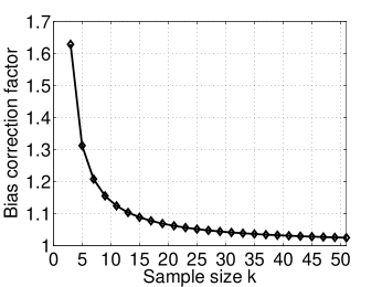
Figure 1: The bias correction factor, $b_{me}$ in (34), as a function of $k=2m+1$. After $k>50$, the bias is negligible. Note that $b_{me}=\infty$ when $k=1$.

The sample median is a special case of sample quantile estimators (Fama and Roll, 1968, 1971). For example, one version of the quantile estimators given by McCulloch (1986) would be

$$\hat{d}_{or}=\frac{\hat{|x|}_{.75}-\hat{|x|}_{.25}}{2.0},$$ (36)

where $\hat{|x|}_{.75}$ and $\hat{|x|}_{.25}$ are the .75 and .25 sample quantiles of $\{|x_{j}|\}_{j=1}^{k}$, respectively.

Our simulations indicate that $\hat{d}_{me}$ actually slightly outperforms $\hat{d}_{or}$. This is not surprising. $\hat{d}_{or}$ works for any Cauchy distribution whose location parameter does not have to be zero, while $\hat{d}_{me}$ takes advantage of the fact that the Cauchy location parameter is always zero in our case.

5 The Geometric Mean Estimators

This section derives estimators based on the geometric mean, which are more accurate than the sample median estimators. The geometric mean estimators allow us to derive tail bounds in explicit forms and (consequently) an analog of the Johnson-Lindenstrauss (JL) lemma for dimension reduction in $l_{1}$.

Recall, our goal is to estimate $d$ from $k$ i.i.d. samples $x_{j}\sim C(0,d)$. To help derive the geometric mean estimators, we first study two nonlinear estimators based on the fractional moment, i.e., $\text{E}(|x|^{\lambda})$ ($|\lambda|<1$) and the logarithmic moment, i.e, $\text{E}\left(\log(|x|)\right)$, respectively, as presented in Lemma 2. See the proof in Appendix B.

Lemma 2

Assume $x\sim C(0,d)$. Then

$$\text{E}\left(|x|^{\lambda}\right)=\frac{d^{\lambda}}{\cos(\lambda\pi/2)},\hskip 36.135pt|\lambda|<1$$ (37)

$$\text{E}\left(\log(|x|)\right)=\log(d),$$ (38)

$$\text{Var}\left(\log(|x|)\right)=\frac{\pi^{2}}{4},$$ (39)

from which we can derive two biased estimators of $d$ from $k$ i.i.d. samples $x_{j}\sim C(0,d)$:

$$\hat{d}_{\lambda}=\left(\frac{1}{k}\sum_{j=1}^{k}|x_{j}|^{\lambda}\cos(\lambda\pi/2)\right)^{1/\lambda},\hskip 14.45377pt|\lambda|<1,$$ (40)

$$\hat{d}_{log}=\exp\left(\frac{1}{k}\sum_{j=1}^{k}\log(|x_{j}|)\right),$$ (41)

whose variances are, respectively,

$$\text{Var}\left(\hat{d}_{\lambda}\right)=\frac{d^{2}}{k}\frac{\sin^{2}(\lambda\pi/2)}{\lambda^{2}\cos(\lambda\pi)}+O\left(\frac{1}{k^{2}}\right),\hskip 14.45377pt|\lambda|<1/2$$ (42)

$$\text{Var}\left(\hat{d}_{log}\right)=\frac{\pi^{2}d^{2}}{4k}+O\left(\frac{1}{k^{2}}\right).$$ (43)

The term $\frac{\sin^{2}(\lambda\pi/2)}{\lambda^{2}\cos(\lambda\pi)}$ decreases with decreasing $|\lambda|$, reaching a limit

$$\underset{\lambda\rightarrow 0}{\lim}\frac{\sin^{2}(\lambda\pi/2)}{\lambda^{2}\cos(\lambda\pi)}=\frac{\pi^{2}}{4}.$$ (44)

In other words, the variance of $\hat{d}_{\lambda}$ converges to that of $\hat{d}_{log}$ as $|\lambda|$ approaches zero.

Note that $\hat{d}_{log}$ can in fact be written as the geometric mean:

$$\hat{d}_{log}=\hat{d}_{gm}=\prod_{j=1}^{k}|x_{j}|^{1/k}.$$ (45)

$\hat{d}_{\lambda}$ is a non-convex norm ($l_{\lambda}$) because $\lambda<1$. $\hat{d}_{gm}$ is also a non-convex norm (the $l_{\lambda}$ norm as $\lambda\rightarrow 0$). Both $\hat{d}_{\lambda}$ and $\hat{d}_{gm}$ do not satisfy the triangle inequality.

We propose $\hat{d}_{gm,c}$, the bias-corrected geometric mean estimator. Lemma 3 derives the moments of $\hat{d}_{gm,c}$, proved in Appendix C.

Lemma 3

$$\hat{d}_{gm,c}=\cos^{k}\left(\frac{\pi}{2k}\right)\prod_{j=1}^{k}|x_{j}|^{1/k},\hskip 7.22743ptk>1$$ (46)

is unbiased, with the variance (valid when $k>2$)

$$\text{Var}\left(\hat{d}_{gm,c}\right) =d^{2}\left(\frac{\cos^{2k}\left(\frac{\pi}{2k}\right)}{\cos^{k}\left(\frac{\pi}{k}\right)}-1\right)=\frac{d^{2}}{k}\frac{\pi^{2}}{4}+\frac{\pi^{4}}{32}\frac{d^{2}}{k^{2}}+O\left(\frac{1}{k^{3}}\right).$$ (47)

The third and fourth central moments are (for $k>3$ and $k>4$, respectively)

$$\text{E}\left(\hat{d}_{gm,c}-\text{E}\left(\hat{d}_{gm,c}\right)\right)^{3}=\frac{3\pi^{4}}{16}\frac{d^{3}}{k^{2}}+O\left(\frac{1}{k^{3}}\right)$$ (48)

$$\text{E}\left(\hat{d}_{gm,c}-\text{E}\left(\hat{d}_{gm,c}\right)\right)^{4}=\frac{3\pi^{4}}{16}\frac{d^{4}}{k^{2}}+O\left(\frac{1}{k^{3}}\right).$$ (49)

The higher (third or fourth) moments may be useful for approximating the distribution of $\hat{d}_{gm,c}$. In Section 6, we will show how to approximate the distribution of the maximum likelihood estimator by matching the first four moments (in the leading terms). We could apply the similar technique to approximate $\hat{d}_{gm,c}$. Fortunately, we do not have to do so because we are able to derive the exact tail bounds of $\hat{d}_{gm,c}$ in Lemma 4, which is proved in Appendix D.

Lemma 4

$$\mathbf{Pr}\left(\hat{d}_{gm,c}\geq(1+\epsilon)d\right)\leq\frac{\cos^{kt_{1}^{*}}\left(\frac{\pi}{2k}\right)}{\cos^{k}\left(\frac{\pi t_{1}^{*}}{2k}\right)(1+\epsilon)^{t_{1}^{*}}},\hskip 18.06749pt\epsilon\geq 0$$ (50)

where

$$t_{1}^{*}=\frac{2k}{\pi}\tan^{-1}\left(\left(\log(1+\epsilon)-k\log\cos\left(\frac{\pi}{2k}\right)\right)\frac{2}{\pi}\right).$$ (51)

$$\mathbf{Pr}\left(\hat{d}_{gm,c}\leq(1-\epsilon)d\right)\leq\frac{(1-\epsilon)^{t_{2}^{*}}}{\cos^{k}\left(\frac{\pi t_{2}^{*}}{2k}\right)\cos^{kt_{2}^{*}}\left(\frac{\pi}{2k}\right)},\hskip 18.06749pt0\leq\epsilon\leq 1,\hskip 7.22743ptk\geq\frac{\pi^{2}}{8\epsilon}$$ (52)

where

$$t_{2}^{*}=\frac{2k}{\pi}\tan^{-1}\left(\left(-\log(1-\epsilon)+k\log\cos\left(\frac{\pi}{2k}\right)\right)\frac{2}{\pi}\right).$$ (53)

By restricting $0\leq\epsilon\leq 1$, the tail bounds can be written in exponential forms:

$$\mathbf{Pr}\left(\hat{d}_{gm,c}\geq(1+\epsilon)d\right)\leq\exp\left(-k\frac{\epsilon^{2}}{8(1+\epsilon)}\right)$$ (54)

$$\mathbf{Pr}\left(\hat{d}_{gm,c}\leq(1-\epsilon)d\right)\leq\exp\left(-k\frac{\epsilon^{2}}{8(1+\epsilon)}\right),\hskip 14.45377ptk\geq\frac{\pi^{2}}{1.5\epsilon}$$ (55)

An analog of the JL bound for $l_{1}$ follows from the exponential tail bounds (54) and (55).

Lemma 5

Using $\hat{d}_{gm,c}$ with $k\geq\frac{8\left(2\log n-\log\delta\right)}{\epsilon^{2}/(1+\epsilon)}\geq\frac{\pi^{2}}{1.5\epsilon}$, then with probability at least $1-\delta$, the $l_{1}$ distance, $d$, between any pair of data points (among $n$ data points), can be estimated with errors bounded by $\pm\epsilon d$, i.e., $|\hat{d}_{gm,c}-d|\leq\epsilon d$.

Remarks on Lemma 5: (1) We can replace the constant “8” in Lemma 5 with better (i.e., smaller) constants for specific values of $\epsilon$. For example, If $\epsilon=0.2$, we can replace “8” by “5”. See the proof of Lemma 4. (2) This Lemma is weaker than the classical JL Lemma for dimension reduction in $l_{2}$ as reviewed in Section 2.1. The classical JL Lemma for $l_{2}$ ensures that the $l_{2}$ inter-point distances of the projected data points are close enough to the original $l_{2}$ distances, while Lemma 5 merely says that the projected data points contain enough information to reconstruct the original $l_{1}$ distances. On the other hand, the geometric mean estimator is a non-convex norm; and therefore it does contain some information about the geometry. We leave it for future work to explore the possibility of developing efficient algorithms using the geometric mean estimator.

Figure 2 presents the simulated histograms of $\hat{d}_{gm,c}$ for $d=1$, with $k=5$ and $k=50$. The histograms reveal some characteristics shared by the maximum likelihood estimator we will discuss in the next section:

• Supported on $[0,\infty)$, $\hat{d}_{gm,c}$ is positively skewed.

• The distribution of $\hat{d}_{gm,c}$ is still “heavy-tailed.” However, in the region not too far from the mean, the distribution of $\hat{d}_{gm,c}$ may be well captured by a gamma (or a generalized gamma) distribution. For large $k$, even a normal approximation may suffice.

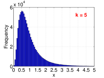
(a) $k=5$

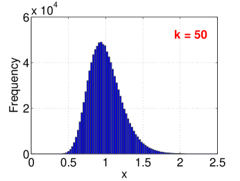
(b) $k=50$

Figure 2: Histograms of $\hat{d}_{gm,c}$, obtained from $10^{6}$ simulations. At least in the range not too far from the mean, the distribution of $\hat{d}_{gm,c}$ resembles a gamma and also resembles a normal when $k$ is large enough.

Figure 3 compares $\hat{d}_{gm,c}$ with the sample median estimators $\hat{d}_{me}$ and $\hat{d}_{me,c}$, in terms of the mean square errors. $\hat{d}_{gm,c}$ is considerably more accurate than $\hat{d}_{me}$ at small $k$. The bias correction significantly reduces the mean square errors of $\hat{d}_{me}$.

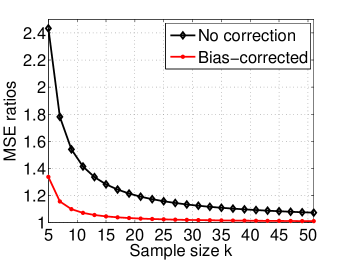
Figure 3: The ratios of the mean square errors (MSN), $\frac{\text{MSE}(\hat{d}_{me})}{\text{MSE}(\hat{d}_{gm,c})}$ and $\frac{\text{MSE}(\hat{d}_{me,c})}{\text{MSE}(\hat{d}_{gm,c})}$, demonstrate that the bias-corrected geometric mean estimator $\hat{d}_{gm,c}$ is considerably more accurate than the sample median estimator $\hat{d}_{me}$. The bias correction on $\hat{d}_{me}$ considerably reduces the MSE. Note that when $k=3$, the ratios are $\infty$.

6 The Maximum Likelihood Estimators

This section is devoted to analyzing the maximum likelihood estimators (MLE), which are “asymptotically optimum.” In comparisons, the sample median estimators and geometric mean estimators are not optimum. Our contribution in this section includes the higher-order analysis for the bias and moments and accurate closed-from approximations to the distribution of the MLE.

The method of maximum likelihood is widely used. For example, Li et al. (2006b) applied the maximum likelihood method to normal random projections and provided an improved estimator of the $l_{2}$ distance by taking advantage of the marginal information.

The Cauchy distribution is often considered a “challenging” example because of the “multiple roots” problem when estimating the location parameter (Barnett, 1966; Haas et al., 1970). In our case, since the location parameter is always zero, much of the difficulty is avoided.

Recall our goal is to estimate $d$ from $k$ i.i.d. samples $x_{j}\sim C(0,d),j=1,2,...,k$. The $\log$ joint likelihood of $\{x_{j}\}_{j=1}^{k}$ is

$$L(x_{1},x_{2},...x_{k};d)=k\log(d)-k\log(\pi)-\sum_{j=1}^{k}\log(x_{j}^{2}+d^{2}),$$ (56)

whose first and second derivatives (w.r.t. $d$) are

$$L^{\prime}(d)=\frac{k}{d}-\sum_{j=1}^{k}\frac{2d}{x_{j}^{2}+d^{2}},$$ (57)

$$L^{\prime\prime}(d)=-\frac{k}{d^{2}}-\sum_{j=1}^{k}\frac{2x_{j}^{2}-2d^{2}}{(x_{j}^{2}+d^{2})^{2}}=-\frac{L^{\prime}(d)}{d}-4\sum_{j=1}^{k}\frac{x_{j}^{2}}{(x_{j}^{2}+d^{2})^{2}}.$$ (58)

The maximum likelihood estimator of $d$, denoted by $\hat{d}_{MLE}$, is the solution to $L^{\prime}(d)=0$, i.e.,

$$-\frac{k}{\hat{d}_{MLE}}+\sum_{j=1}^{k}\frac{2\hat{d}_{MLE}}{x_{j}^{2}+\hat{d}_{MLE}^{2}}=0.$$ (59)

Because $L^{\prime\prime}(\hat{d}_{MLE})\leq 0$, $\hat{d}_{MLE}$ indeed maximizes the joint likelihood and is the only solution to the MLE equation (59). Solving (59) numerically is not difficult (e.g., a few iterations using the Newton’s method). For a better accuracy, we recommend the following bias-corrected estimator:

$$\hat{d}_{MLE,c}=\hat{d}_{MLE}\left(1-\frac{1}{k}\right).$$ (60)

Lemma 6 concerns the asymptotic moments of $\hat{d}_{MLE}$ and $\hat{d}_{MLE,c}$, proved in Appendix E.

Lemma 6

Both $\hat{d}_{MLE}$ and $\hat{d}_{MLE,c}$ are asymptotically unbiased and normal. The first four moments of $\hat{d}_{MLE}$ are

$$\text{E}\left(\hat{d}_{MLE}-d\right)=\frac{d}{k}+O\left(\frac{1}{k^{2}}\right)$$ (61)

$$\text{Var}\left(\hat{d}_{MLE}\right)=\frac{2d^{2}}{k}+\frac{7d^{2}}{k^{2}}+O\left(\frac{1}{k^{3}}\right)$$ (62)

$$\text{E}\left(\hat{d}_{MLE}-\text{E}(\hat{d}_{MLE})\right)^{3}=\frac{12d^{3}}{k^{2}}+O\left(\frac{1}{k^{3}}\right)$$ (63)

$$\text{E}\left(\hat{d}_{MLE}-\text{E}(\hat{d}_{MLE})\right)^{4}=\frac{12d^{4}}{k^{2}}+\frac{222d^{4}}{k^{3}}+O\left(\frac{1}{k^{4}}\right)$$ (64)

The first four moments of $\hat{d}_{MLE,c}$ are

$$\text{E}\left(\hat{d}_{MLE,c}-d\right)=O\left(\frac{1}{k^{2}}\right)$$ (65)

$$\text{Var}\left(\hat{d}_{MLE,c}\right)=\frac{2d^{2}}{k}+\frac{3d^{2}}{k^{2}}+O\left(\frac{1}{k^{3}}\right)$$ (66)

$$\text{E}\left(\hat{d}_{MLE,c}-\text{E}(\hat{d}_{MLE,c})\right)^{3}=\frac{12d^{3}}{k^{2}}+O\left(\frac{1}{k^{3}}\right)$$ (67)

$$\text{E}\left(\hat{d}_{MLE,c}-\text{E}(\hat{d}_{MLE,c})\right)^{4}=\frac{12d^{4}}{k^{2}}+\frac{186d^{4}}{k^{3}}+O\left(\frac{1}{k^{4}}\right)$$ (68)

The order $O\left(\frac{1}{k}\right)$ term of the variance, i.e., $\frac{2d^{2}}{k}$, is known, e.g., (Haas et al., 1970). We derive the bias-corrected estimator, $\hat{d}_{MLE,c}$, and the higher order moments using stochastic Taylor expansions (Bartlett, 1953; Shenton and Bowman, 1963; Ferrari et al., 1996; Cysneiros et al., 2001).

We will propose an inverse Gaussian distribution to approximate the distribution of $\hat{d}_{MLE,c}$, by matching the first four moments (at least in the leading terms).

6.1 A Numerical Example

The maximum likelihood estimators are tested on MSN Web crawl data, a term-by-document matrix with $D=2^{16}$ Web pages. We conduct Cauchy random projections and estimate the $l_{1}$ distances between words. In this experiment, we compare the empirical and (asymptotic) theoretical moments, using one pair of words. Figure 4 illustrates that the bias correction is effective and these (asymptotic) formulas for the first four moments of $\hat{d}_{MLE,c}$ in Lemma 6 are accurate, especially when $k\geq 20$.

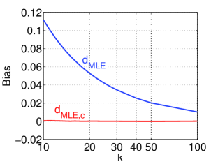
(a) $\text{E}(\hat{d}_{MLE}-d)/d$ v.s. $\text{E}(\hat{d}_{MLE,c}-d)/d$

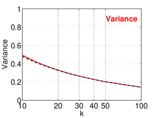
(b) $\left(\text{E}(\hat{d}_{MLE,c}-\text{E}(\hat{d}_{MLE,c}))^{2}/d^{2}\right)^{1/2}$

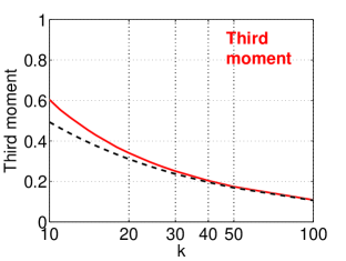
(c) $\left(\text{E}(\hat{d}_{MLE,c}-\text{E}(\hat{d}_{MLE,c}))^{3}/d^{3}\right)^{1/3}$

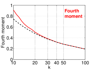
(d) $\left(\text{E}(\hat{d}_{MLE,c}-\text{E}(\hat{d}_{MLE,c}))^{4}/d^{4}\right)^{1/4}$

Figure 4: One pair of words are selected from an MSN term-by-document matrix with $D=2^{16}$ Web pages. We conduct Cauchy random projections and estimate the $l_{1}$ distance between one pair of words using the maximum likelihood estimator $\hat{d}_{MLE}$ and the bias-corrected version $\hat{d}_{MLE,c}$. Panel (a) plots the biases of $\hat{d}_{MLE}$ and $\hat{d}_{MLE,c}$, indicating that the bias correction is effective. Panels (b), (c), and (d) plot the variance, third moment, and fourth moment of $\hat{d}_{MLE,c}$, respectively. The dashed curves are the theoretical asymptotic moments. When $k\geq 20$, the theoretical asymptotic formulas for moments are accurate.

6.2 Approximation Distributions

Theoretical analysis on the exact distribution of a maximum likelihood estimator is difficult. In statistics, the standard approach is to assume normality, which, however, is quite inaccurate. The so-called Edgeworth expansion improves the normal approximation by matching higher moments (Feller, 1971; Bhattacharya and Ghosh, 1978; Severini, 2000). For example, if we approximate the distribution of $\hat{d}_{MLE,c}$ using an Edgeworth expansion by matching the first four moments of $\hat{d}_{MLE,c}$ derived in Lemma 6, then the errors will be on the order of $O\left(k^{-3/2}\right)$. However, Edgeworth expansions have some well-known drawbacks. The resultant expressions are quite sophisticated. They are not accurate at the tails. It is possible that the approximate probability has values below zero. Also, Edgeworth expansions consider the support is $(-\infty,\infty)$, while $\hat{d}_{MLE,c}$ is non-negative.

We propose approximating the distributions of $\hat{d}_{MLE,c}$ directly using some well-studied common distributions. We will first consider a gamma distribution with the same first two (asymptotic) moments of $\hat{d}_{MLE,c}$. That is, the gamma distribution will be asymptotically equivalent to the normal approximation. While a normal has zero third central moment, a gamma has nonzero third central moment. This, to an extent, speeds up the rate of convergence. Another important reason why a gamma is more accurate is because it has the same support as $\hat{d}_{MLE,c}$, i.e., $[0,\infty)$.

We will furthermore consider a generalized gamma distribution, which allows us to match the first three (asymptotic) moments of $\hat{d}_{MLE,c}$. Interestingly, in this case, the generalized gamma approximation turns out to be an inverse Gaussian distribution, which has a closed-form probability density. More interestingly, this inverse Gaussian distribution also matches the fourth central moment of $\hat{d}_{MLE,c}$ in the $O\left(\frac{1}{k^{2}}\right)$ term and almost in the $O\left(\frac{1}{k^{3}}\right)$ term. By simulations, the inverse Gaussian approximation is highly accurate.

Note that, since we are interested in the very small (e.g., $10^{-10}$) tail probability range, $O\left(k^{-3/2}\right)$ is not too meaningful. For example, $k^{-3/2}=10^{-3}$ if $k=100$. Therefore, we will have to rely on simulations to assess the accuracy of the approximations. On the other hand, an upper bound may hold exactly (verified by simulations) even if it is based on an approximate distribution.

As the related work, Li et al. (2006e) applied gamma and generalized gamma approximations to model the performance measure distribution in some wireless communication channels using random matrix theory and produced accurate results in evaluating the error probabilities.

6.2.1 The Gamma Approximation

The gamma approximation is an obvious improvement over the normal approximation. A gamma distribution, $G(\alpha,\beta)$, has two parameters, $\alpha$ and $\beta$, which can be determined by matching the first two (asymptotic) moments of $\hat{d}_{MLE,c}$. That is, we assume that $\hat{d}_{MLE,c}\sim G(\alpha,\beta)$, with

$$\alpha\beta=d,\hskip 18.06749pt\alpha\beta^{2}=\frac{2d^{2}}{k}+\frac{3d^{2}}{k^{2}},\ \ \ \Longrightarrow\ \ \alpha=\frac{1}{\frac{2}{k}+\frac{3}{k^{2}}},\hskip 18.06749pt\beta=\frac{2d}{k}+\frac{3d}{k^{2}}.$$ (69)

Assuming a gamma distribution, it is easy to obtain the following Chernoff bounds:

$$\mathbf{Pr}\left(\hat{d}_{MLE,c}\geq(1+\epsilon)d\right)\overset{\sim}{\leq}\exp\left(-\alpha\left(\epsilon-\log(1+\epsilon)\right)\right),\hskip 14.45377pt\epsilon\geq 0$$ (70)

$$\mathbf{Pr}\left(\hat{d}_{MLE,c}\leq(1-\epsilon)d\right)\overset{\sim}{\leq}\exp\left(-\alpha\left(-\epsilon-\log(1-\epsilon)\right)\right),\hskip 14.45377pt0\leq\epsilon<1,$$ (71)

where we use $\overset{\sim}{\leq}$ to indicate that these inequalities are based on an approximate distribution.

Note that the distribution of $\hat{d}_{MLE}/d$ (and hence $\hat{d}_{MLE,c}/d$) is only a function of $k$ as shown in (Antle and Bain, 1969; Haas et al., 1970). Therefore, we can evaluate the accuracy of the gamma approximation by simulations with $d=1$, as presented in Figure 5.

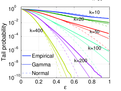
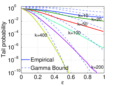
Figure 5: We consider $k$ = 10, 20, 50, 100, 200, and 400. For each $k$, we simulate standard Cauchy samples, from which we estimate the Cauchy parameter by the MLE $\hat{d}_{MLE,c}$ and compute the tail probabilities. Panel (a) compares the empirical tail probabilities (thick solid) with the gamma tail probabilities (thin solid), indicating that the gamma distribution is better than the normal (dashed) for approximating the distribution of $\hat{d}_{MLE,c}$. Panel (b) compares the empirical tail probabilities with the gamma upper bound (70)+(71).

Figure 5(a) shows that both the gamma and normal approximations are fairly accurate when the tail probability $\geq 10^{-2}\sim 10^{-3}$; and the gamma approximation is obviously better.

Figure 5(b) compares the empirical tail probabilities with the gamma Chernoff upper bound (70)+(71), indicating that these bounds are reliable, when the tail probability $\geq 10^{-5}\sim 10^{-6}$.

6.2.2 The Inverse Gaussian (Generalized Gamma) Approximation

The distribution of $\hat{d}_{MLE,c}$ can be well approximated by an inverse Gaussian distribution, which is a special case of the three-parameter generalized gamma distribution (Hougaard, 1986; Gerber, 1991), denoted by $GG(\alpha,\beta,\eta)$. Note that the usual gamma distribution is a special case with $\eta=1$.

If $z\sim GG(\alpha,\beta,\eta)$, then the first three moments are

$$\text{E}(z)=\alpha\beta,\hskip 14.45377pt\text{Var}(z)=\alpha\beta^{2},\hskip 14.45377pt\text{E}\left(z-\text{E}(z)\right)^{3}=\alpha\beta^{3}(1+\eta).$$ (72)

We can approximate the distribution of $\hat{d}_{MLE,c}$ by matching the first three moments, i.e.,

$$\alpha\beta=d,\hskip 14.45377pt\alpha\beta^{2}=\frac{2d^{2}}{k}+\frac{3d^{2}}{k^{2}},\hskip 14.45377pt\alpha\beta^{3}(1+\eta)=\frac{12d^{3}}{k^{2}},$$ (73)

from which we obtain

$$\alpha=\frac{1}{\frac{2}{k}+\frac{3}{k^{2}}},\hskip 14.45377pt\beta=\frac{2d}{k}+\frac{3d}{k^{2}},\hskip 14.45377pt\eta=2+O\left(\frac{1}{k}\right).$$ (74)

Taking only the leading term for $\eta$, the generalized gamma approximation of $\hat{d}_{MLE,c}$ would be

$$GG\left(\frac{1}{\frac{2}{k}+\frac{3}{k^{2}}},\frac{2d}{k}+\frac{3d}{k^{2}},2\right).$$ (75)

In general, a generalized gamma distribution does not have a closed-form density function although it always has a closed-from moment generating function. In our case, (75) is actually an inverse Gaussian distribution, which has a closed-form density function. Assuming $\hat{d}_{MLE,c}\sim IG(\alpha,\beta)$, with parameters $\alpha$ and $\beta$ defined in (74), the moment generating function (MGF), the probability density function (PDF), and cumulative density function (CDF) would be (Seshadri, 1993, Chapter 2) (Tweedie, 1957a, b)

$$\text{E}\left(\exp(\hat{d}_{MLE,c}t)\right)\overset{\sim}{=}\exp\left(\alpha\left(1-(1-2\beta t)^{1/2}\right)\right),$$ (76)

$$\mathbf{Pr}(\hat{d}_{MLE,c}=y)\overset{\sim}{=}\frac{\alpha\sqrt{\beta}}{\sqrt{2\pi}}y^{-\frac{3}{2}}\exp\left(-\frac{\left(y/\beta-\alpha\right)^{2}}{2y/\beta}\right)=\sqrt{\frac{\alpha d}{2\pi}}y^{-\frac{3}{2}}\exp\left(-\frac{\left(y-d\right)^{2}}{2y\beta}\right),$$ (77)

$$\mathbf{Pr}\left(\hat{d}_{MLE,c}\leq y\right)\overset{\sim}{=}\Phi\left(\sqrt{\frac{\alpha^{2}\beta}{y}}\left(\frac{y}{\alpha\beta}-1\right)\right)+e^{2\alpha}\Phi\left(-\sqrt{\frac{\alpha^{2}\beta}{y}}\left(\frac{y}{\alpha\beta}+1\right)\right)$$

$$\hskip 79.49744pt=\Phi\left(\sqrt{\frac{\alpha d}{y}}\left(\frac{y}{d}-1\right)\right)+e^{2\alpha}\Phi\left(-\sqrt{\frac{\alpha d}{y}}\left(\frac{y}{d}+1\right)\right),$$ (78)

where $\Phi(.)$ is the standard normal CDF, i.e., $\Phi(z)=\int_{-\infty}^{z}\frac{1}{\sqrt{2\pi}}e^{-\frac{t^{2}}{2}}dt$. Here we use $\overset{\sim}{=}$ to indicate that these equalities are based on an approximate distribution.

Assuming $\hat{d}_{MLE,c}\sim IG(\alpha,\beta)$, then the fourth central moment should be

$$\text{E}\left(\hat{d}_{MLE,c}-\text{E}\left(\hat{d}_{MLE,c}\right)\right)^{4} \overset{\sim}{=}15\alpha\beta^{4}+3\left(\alpha\beta^{2}\right)^{2}$$

$$=15d\left(\frac{2d}{k}+\frac{3d}{k^{2}}\right)^{3}+3\left(\frac{2d^{2}}{k}+\frac{3d^{2}}{k^{2}}\right)^{2}$$

$$=\frac{12d^{4}}{k^{2}}+\frac{156d^{4}}{k^{3}}+O\left(\frac{1}{k^{4}}\right).$$ (79)

Lemma 6 has shown the true asymptotic fourth central moment:

$$\text{E}\left(\hat{d}_{MLE,c}-\text{E}\left(\hat{d}_{MLE,c}\right)\right)^{4}=\frac{12d^{4}}{k^{2}}+\frac{186d^{4}}{k^{3}}+O\left(\frac{1}{k^{4}}\right).$$ (80)

That is, the inverse Gaussian approximation matches not only the leading term, $\frac{12d^{4}}{k^{2}}$, but also almost the higher order term, $\frac{186d^{4}}{k^{3}}$, of the true asymptotic fourth moment of $\hat{d}_{MLE,c}$.

Assuming $\hat{d}_{MLE,c}\sim IG(\alpha,\beta)$, the tail probability of $\hat{d}_{MLE,c}$ can be expressed as

$$\mathbf{Pr}\left(\hat{d}_{MLE,c}\geq(1+\epsilon)d\right)\overset{\sim}{=}\Phi\left(-\epsilon\sqrt{\frac{\alpha}{1+\epsilon}}\right)-e^{2\alpha}\Phi\left(-(2+\epsilon)\sqrt{\frac{\alpha}{1+\epsilon}}\right),\hskip 7.22743pt\epsilon\geq 0$$ (81)

$$\mathbf{Pr}\left(\hat{d}_{MLE,c}\leq(1-\epsilon)d\right)\overset{\sim}{=}\Phi\left(-\epsilon\sqrt{\frac{\alpha}{1-\epsilon}}\right)+e^{2\alpha}\Phi\left(-(2-\epsilon)\sqrt{\frac{\alpha}{1-\epsilon}}\right),\hskip 7.22743pt0\leq\epsilon<1.$$ (82)

Assuming $\hat{d}_{MLE,c}\sim IG(\alpha,\beta)$, it is easy to show the following Chernoff bounds:

$$\mathbf{Pr}\left(\hat{d}_{MLE,c}\geq(1+\epsilon)d\right)\overset{\sim}{\leq}\exp\left(-\frac{\alpha\epsilon^{2}}{2(1+\epsilon)}\right),\hskip 14.45377pt\epsilon\geq 0$$ (83)

$$\mathbf{Pr}\left(\hat{d}_{MLE,c}\leq(1-\epsilon)d\right)\overset{\sim}{\leq}\exp\left(-\frac{\alpha\epsilon^{2}}{2(1-\epsilon)}\right),\hskip 14.45377pt0\leq\epsilon<1.$$ (84)

To see (83). Assume $z\sim IG(\alpha,\beta)$. Then, using the Chernoff inequality:

$$\mathbf{Pr}\left(z\geq(1+\epsilon)d\right)\leq \text{E}\left(zt\right)\exp(-(1+\epsilon)dt)$$

$$= \exp\left(\alpha\left(1-(1-2\beta t)^{1/2}\right)-(1+\epsilon)dt\right),$$

whose minimum is $\exp\left(-\frac{\alpha\epsilon^{2}}{2(1+\epsilon)}\right)$, attained at $t=\left(1-\frac{1}{(1+\epsilon)^{2}}\right)\frac{1}{2\beta}$. We can similarly show (84).

Combining (83) and (84) yields a symmetric bound

$$\mathbf{Pr}\left(|\hat{d}_{MLE,c}-d|\geq\epsilon d\right)\overset{\sim}{\leq}2\exp\left(-\frac{\epsilon^{2}/(1+\epsilon)}{2\left(\frac{2}{k}+\frac{3}{k^{2}}\right)}\right),\hskip 10.84006pt0\leq\epsilon\leq 1$$ (85)

Figure 6 compares the inverse Gaussian approximation with the same simulations as presented in Figure 5, indicating that the inverse Gaussian approximation is highly accurate. When the tail probability $\geq 10^{-4}\sim 10^{-6}$, we can treat the inverse Gaussian as the exact distribution of $\hat{d}_{MLE,c}$. The Chernoff upper bounds for the inverse Gaussian are always reliable in our simulation range (the tail probability $\geq 10^{-10}$).

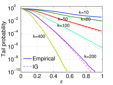
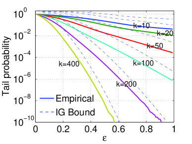
Figure 6: We compare the inverse Gaussian approximation with the same simulations as presented in Figure 5. Panel (a) compares the empirical tail probabilities with the inverse Gaussian tail probabilities, indicating that the approximation is highly accurate. Panel (b) compares the empirical tail probabilities with the inverse Gaussian upper bound (83)+(84). The upper bounds are all above the corresponding empirical curves, indicating that our proposed bounds are reliable at least in our simulation range.

7 Conclusion

It is well-known that the $l_{1}$ distance is far more robust than the $l_{2}$ distance against “outliers.” There are numerous success stories of using the $l_{1}$ distance, e.g., Lasso (Tibshirani, 1996), LARS (Efron et al., 2004), 1-norm SVM (Zhu et al., 2003), and Laplacian radial basis kernel (Chapelle et al., 1999; Ferecatu et al., 2004).

Dimension reduction in the $l_{1}$ norm, however, has been proved impossible if we use linear random projections and linear estimators. In this study, we propose three types of nonlinear estimators for Cauchy random projections: the bias-corrected sample median estimator, the bias-corrected geometric mean estimator, and the bias-corrected maximum likelihood estimator. Our theoretical analysis has shown that these nonlinear estimators can accurately recover the original $l_{1}$ distance, even though none of them can be a metric.

The bias-corrected sample median estimator and the bias-corrected geometric mean estimator are asymptotically equivalent but the latter is more accurate at small sample size. We have derived explicit tail bounds for the bias-corrected geometric mean estimator and have expressed the tail bounds in exponential forms. Using these tail bounds, we have established an analog of the Johnson-Lindenstrauss (JL) lemma for dimension reduction in $l_{1}$, which is weaker than the classical JL lemma for dimension reduction in $l_{2}$.

We conduct theoretic analysis on the bias-corrected maximum likelihood estimator (MLE), which is “asymptotically optimum.” Both the sample median estimator and the geometric mean estimator are about $80\%$ efficient as the MLE. We propose approximating its distribution by an inverse Gaussian, which has the same support and matches the leading terms of the first four moments of the proposed estimator. Approximate tail bounds have been provide based on the inverse Gaussian approximation. Verified by simulations, these approximate tail bounds hold at least in the $\geq 10^{-10}$ tail probability range.

Although these nonlinear estimators are not metrics, they are still useful for certain applications in (e.g.,) data stream computation, information retrieval, learning and data mining, whenever the goal is to compute the $l_{1}$ distances efficiently using a small storage space.

The geometric mean estimator is a non-convex norm (i.e., the $l_{p}$ norm as $p\rightarrow 0$); and therefore it does contain some information about the geometry. It may be still possible to develop certain efficient algorithms using the geometric mean estimator by avoiding the non-convexity. We leave this for future work.

A Proof of Lemma 1

Assume $x\sim C(0,d)$. The probability density function (PDF) and the cumulative density function (CDF) of $|x|$ would be

$$\mathbf{Pr}(|x|=z)=\frac{2d}{\pi}\frac{1}{z^{2}+d^{2}},\hskip 14.45377ptz\geq 0$$ (86)

$$\mathbf{Pr}(|x|\leq z)=\frac{2}{\pi}\tan^{-1}\frac{z}{d},\hskip 14.45377ptz\geq 0$$ (87)

The asymptotic normality of $\hat{d}_{me}$ follows from the asymptotic results on sample quantiles (Shao, 2003, Theorem 5.10).

$$\sqrt{k}\left(\hat{d}_{me}-d\right)\overset{D}{\Longrightarrow}N\left(0,\frac{1}{2}\left(1-\frac{1}{2}\right)/\left(\left.\mathbf{Pr}(|x|=z)\right|_{z=d}\right)^{2}\right)=N\left(0,\frac{\pi^{2}}{4}d^{2}\right)$$ (88)

The probability density of $\hat{d}_{me}$ can be derived from the probability density of order statistics (Shao, 2003, Example 2.9). For simplicity, we only consider $k=2m+1$, $m=1,2,...,$

$$\mathbf{Pr}(\hat{d}_{me}=z) =\frac{(2m+1)!}{(m!)^{2}}\left(\mathbf{Pr}(|x|\leq z)\right)^{m}\left(1-\mathbf{Pr}(|x|\leq z)\right)^{m}\mathbf{Pr}(|x|=z)$$

$$=\frac{(2m+1)!}{(m!)^{2}}\left(\frac{2}{\pi}\tan^{-1}\frac{z}{d}\right)^{m}\left(1-\frac{2}{\pi}\tan^{-1}\frac{z}{d}\right)^{m}\frac{2d}{\pi}\frac{1}{z^{2}+d^{2}}.$$ (89)

The $r^{th}$ moment of $\hat{d}_{me}$ would be

$$\text{E}\left(\hat{d}_{me}\right)^{r} =\int_{0}^{\infty}z^{r}\frac{(2m+1)!}{(m!)^{2}}\left(\frac{2}{\pi}\tan^{-1}\frac{z}{d}\right)^{m}\left(1-\frac{2}{\pi}\tan^{-1}\frac{z}{d}\right)^{m}\frac{2d}{\pi}\frac{1}{z^{2}+d^{2}}dz$$

$$=d^{r}\int_{0}^{1}\frac{(2m+1)!}{(m!)^{2}}\tan^{r}\left(\frac{\pi}{2}t\right)\left(t-t^{2}\right)^{m}dt,$$ (90)

by substituting $t=\frac{2}{\pi}\tan^{-1}\frac{z}{d}$.

When $t\rightarrow 1-0$, $\tan\left(\frac{\pi}{2}t\right)\rightarrow\infty$, but $t-t^{2}=t(1-t)\rightarrow 0$. Around $t=1-0$, $\tan\left(\frac{\pi}{2}t\right)=\frac{1}{\tan\left(\frac{\pi}{2}(1-t)\right)}=\frac{2}{\pi}\frac{1}{1-t}+...$, by the Taylor expansion. Therefore, in order for $\text{E}\left(\hat{d}_{me}\right)^{r}<\infty$, we must have $m\geq r$.

We complete the proof of Lemma 1.

B Proof of Lemma 2

Assume $x\sim C(0,d)$. The first moment of $\log(|x|)$ would be

$$\text{E}\left(\log(|x|)\right) =\frac{2d}{\pi}\int_{0}^{\infty}\frac{\log(y)}{y^{2}+d^{2}}dy$$

$$=\frac{1}{\pi}\int_{0}^{\infty}\frac{\log(d)y^{-1/2}}{y+1}+\frac{1/2\log(y)y^{-1/2}}{y+1}dy$$

$$=\log(d),$$ (91)

with the help of the integral tables (Gradshteyn and Ryzhik, 1994, 3.221.1, 4.251.1).

Thus, given i.i.d. samples $x_{j}\sim C(0,d)$, $j=1,2,...,k$, a nonlinear estimator of $d$ would be

$$\hat{d}_{log}=\exp\left(\frac{1}{k}\sum_{j=1}^{k}\log(|x_{j}|)\right).$$ (92)

We can derive another nonlinear estimator from $\text{E}\left(|x|^{\lambda}\right)$, $|\lambda|<1$. Using the integral tables (Gradshteyn and Ryzhik, 1994, 3.221.1), we obtain

$$\text{E}\left(|x|^{\lambda}\right) =\frac{2d}{\pi}\int_{0}^{\infty}\frac{y^{\lambda}}{y^{2}+d^{2}}dy$$

$$=\frac{d^{\lambda}}{\pi}\int_{0}^{\infty}\frac{y^{\frac{\lambda-1}{2}}}{y+1}dy$$

$$=\frac{d^{\lambda}}{\cos(\lambda\pi/2)},$$ (93)

from which a nonlinear estimator follows immediately

$$\hat{d}_{\lambda}=\left(\frac{1}{k}\sum_{j=1}^{k}|x_{j}|^{\lambda}\cos(\lambda\pi/2)\right)^{1/\lambda},\hskip 14.45377pt|\lambda|<1$$ (94)

Both nonlinear estimators $\hat{d}_{log}$ and $\hat{d}_{\lambda}$ are biased. The leading terms of their variances can be obtained by the Delta Method (Shao, 2003, Corollary 1.1).

With the help of (Gradshteyn and Ryzhik, 1994, 4.261.10), we obtain

$$\text{E}\left(\log^{2}(|x|)\right)=\log^{2}(d)+\frac{\pi^{2}}{4},\hskip 14.45377pt\text{i.e., }\ \ \text{Var}\left(\log^{2}(|x|)\right)=\frac{\pi^{2}}{4}.$$ (95)

Thus,

$$\text{E}\left(\frac{1}{k}\sum_{j=1}^{k}\log(|x_{j}|)\right)=\log d,\hskip 36.135pt\text{Var}\left(\frac{1}{k}\sum_{j=1}^{k}\log(|x_{j}|)\right)=\frac{1}{k}\frac{\pi^{2}}{4}.$$ (96)

By the Delta Method, the asymptotic variance of $\hat{d}_{log}$ should be

$$\text{Var}\left(\hat{d}_{log}\right)=\frac{1}{k}\frac{\pi^{2}}{4}\exp^{2}\left(\log(d)\right)+O\left(\frac{1}{k^{2}}\right)=\frac{\pi^{2}d^{2}}{4k}+O\left(\frac{1}{k^{2}}\right).$$ (97)

Similarly, the asymptotic variance of $\hat{d}_{\lambda}$ is

$$\text{Var}\left(\hat{d}_{\lambda}\right)=\frac{d^{2}}{k}\frac{\sin^{2}(\lambda\pi/2)}{\lambda^{2}\cos(\lambda\pi)}+O\left(\frac{1}{k^{2}}\right),\hskip 14.45377pt|\lambda|<1/2$$ (98)

$\text{Var}\left(\hat{d}_{\lambda}\right)\rightarrow\infty$ as $|\lambda|\rightarrow\frac{1}{2}$. $\text{Var}\left(\hat{d}_{\lambda}\right)$ converges to $\text{Var}\left(\hat{d}_{log}\right)$ as $\lambda\rightarrow 0$, because

$$\underset{\lambda\rightarrow 0}{\lim}\frac{\sin^{2}(\lambda\pi/2)}{\lambda^{2}\cos(\lambda\pi)}=\frac{\pi^{2}}{4}.$$ (99)

This completes the proof of Lemma 2.

C Proof of Lemma 3

Assume that $x_{1}$, $x_{2}$, …, $x_{k}$, are i.i.d. $C(0,d)$. The estimator, $\hat{d}_{gm,c}$, expressed as

$$\hat{d}_{gm,c}=\cos^{k}\left(\frac{\pi}{2k}\right)\prod_{j=1}^{k}|x_{j}|^{1/k},$$ (100)

is unbiased, because, from Lemma 2,

$$\text{E}\left(\hat{d}_{gm,c}\right) =\cos^{k}\left(\frac{\pi}{2k}\right)\prod_{j=1}^{k}\text{E}\left(|x_{j}|^{1/k}\right)$$

$$=\cos^{k}\left(\frac{\pi}{2k}\right)\prod_{j=1}^{k}\left(\frac{d^{1/k}}{\cos\left(\frac{\pi}{2k}\right)}\right)$$

$$=d.$$ (101)

The variance is

$$\text{Var}\left(\hat{d}_{gm,c}\right) =\cos^{2k}\left(\frac{\pi}{2k}\right)\prod_{j=1}^{k}\text{E}\left(|x_{j}|^{2/k}\right)-d^{2}$$

$$=d^{2}\left(\frac{\cos^{2k}\left(\frac{\pi}{2k}\right)}{\cos^{k}\left(\frac{\pi}{k}\right)}-1\right)$$ (102)

$$=\frac{\pi^{2}}{4}\frac{d^{2}}{k}+\frac{\pi^{4}}{32}\frac{d^{2}}{k^{2}}+O\left(\frac{1}{k^{3}}\right),$$ (103)

because

$$\frac{\cos^{2k}\left(\frac{\pi}{2k}\right)}{\cos^{k}\left(\frac{\pi}{k}\right)} =\left(\frac{1}{2}+\frac{1}{2}\left(\frac{1}{\cos(\pi/k)}\right)\right)^{k}$$

$$=\left(1+\frac{1}{4}\frac{\pi^{2}}{k^{2}}+\frac{5}{48}\frac{\pi^{4}}{k^{4}}+O\left(\frac{1}{k^{6}}\right)\right)^{k}$$

$$=1+k\left(\frac{1}{4}\frac{\pi^{2}}{k^{2}}+\frac{5}{48}\frac{\pi^{4}}{k^{4}}\right)+\frac{k(k-1)}{2}\left(\frac{1}{4}\frac{\pi^{2}}{k^{2}}+\frac{5}{48}\frac{\pi^{4}}{k^{4}}\right)^{2}+...$$

$$=1+\frac{\pi^{2}}{4}\frac{1}{k}+\frac{\pi^{4}}{32}\frac{1}{k^{2}}+O\left(\frac{1}{k^{3}}\right).$$ (104)

Some more algebra can similarly show the third and fourth central moments:

$$\text{E}\left(\hat{d}_{gm,c}-\text{E}\left(\hat{d}_{gm,c}\right)\right)^{3}=\frac{3\pi^{4}}{16}\frac{d^{3}}{k^{2}}+O\left(\frac{1}{k^{3}}\right)$$ (105)

$$\text{E}\left(\hat{d}_{gm,c}-\text{E}\left(\hat{d}_{gm,c}\right)\right)^{4}=\frac{3\pi^{4}}{16}\frac{d^{4}}{k^{2}}+O\left(\frac{1}{k^{3}}\right).$$ (106)

Therefore, we have completed the proof of Lemma 3.

D Proof of Lemma 4

This section proves the tail bounds for $\hat{d}_{gm,c}$. Note that $\hat{d}_{gm,c}$ does not have a moment generating function because $\text{E}\left(\hat{d}_{gm,c}\right)^{t}=\infty$ if $t\geq k$. However, we can still use the Markov moment bound.

For any $\epsilon\geq 0$ and $0\leq t<k$, the Markov inequality says

$$\mathbf{Pr}\left(\hat{d}_{gm,c}\geq(1+\epsilon)d\right)\leq\frac{\text{E}\left(\hat{d}_{gm,c}\right)^{t}}{(1+\epsilon)^{t}d^{t}}=\frac{\cos^{kt}\left(\frac{\pi}{2k}\right)}{\cos^{k}\left(\frac{\pi t}{2k}\right)(1+\epsilon)^{t}},$$ (107)

which can be minimized by choosing the optimum $t=t_{1}^{*}$, where

$$t_{1}^{*}=\frac{2k}{\pi}\tan^{-1}\left(\left(\log(1+\epsilon)-k\log\cos\left(\frac{\pi}{2k}\right)\right)\frac{2}{\pi}\right).$$ (108)

We need to make sure that $0\leq t_{1}^{*}<k$. $t_{1}^{*}\geq 0$ because $\log\cos(.)\leq 0$; and $t_{1}^{*}<k$ because $\tan^{-1}(.)\leq\frac{\pi}{2}$, with equality holding only when $k\rightarrow\infty$.

For $0\leq\epsilon\leq 1$, we can prove an exponential bound for $\mathbf{Pr}\left(\hat{d}_{gm,c}\geq(1+\epsilon)d\right)$. First of all, note that we do not have to choose the optimum $t=t_{1}^{*}$. By the Taylor expansion, for small $\epsilon$, $t_{1}^{*}$ can be well approximated by

$$t_{1}^{*}\approx\frac{4k\epsilon}{\pi^{2}}+\frac{1}{2}\approx\frac{4k\epsilon}{\pi^{2}}=t_{1}^{**}.$$ (109)

Therefore, taking $t=t_{1}^{**}=\frac{4k\epsilon}{\pi^{2}}$, the tail bound becomes

$$\mathbf{Pr}\left(\hat{d}_{gm,c}\geq(1+\epsilon)d\right) \leq\frac{\cos^{kt_{1}^{**}}\left(\frac{\pi}{2k}\right)}{\cos^{k}\left(\frac{\pi t_{1}^{**}}{2k}\right)(1+\epsilon)^{t_{1}^{**}}}$$

$$=\left(\frac{\cos^{t_{1}^{**}}\left(\frac{\pi}{2k}\right)}{\cos\left(\frac{2\epsilon}{\pi}\right)(1+\epsilon)^{4\epsilon/\pi^{2}}}\right)^{k}$$

$$\leq\left(\frac{1}{\cos\left(\frac{2\epsilon}{\pi}\right)(1+\epsilon)^{4\epsilon/\pi^{2}}}\right)^{k}$$

$$=\exp\left(-k\left(\log\left(\cos\left(\frac{2\epsilon}{\pi}\right)\right)+\frac{4\epsilon}{\pi^{2}}\log(1+\epsilon)\right)\right)$$

$$\leq\exp\left(-k\frac{\epsilon^{2}}{8(1+\epsilon)}\right),\hskip 7.22743pt0\leq\epsilon\leq 1$$ (110)

The last step in (110) needs some explanations. First, by the Taylor expansion,

$$\log\left(\cos\left(\frac{2\epsilon}{\pi}\right)\right)+\frac{4\epsilon}{\pi^{2}}\log(1+\epsilon)$$

$$= \left(-\frac{2\epsilon^{2}}{\pi^{2}}-\frac{4}{3}\frac{\epsilon^{4}}{\pi^{4}}+...\right)+\frac{4\epsilon}{\pi^{2}}\left(\epsilon-\frac{1}{2}\epsilon^{2}+...\right)$$

$$= \frac{2\epsilon^{2}}{\pi^{2}}\left(1-\epsilon+...\right)$$ (111)

Therefore, we can seek the smallest constant $\gamma_{1}$ so that

$$\log\left(\cos\left(\frac{2\epsilon}{\pi}\right)\right)+\frac{4\epsilon}{\pi^{2}}\log(1+\epsilon)\geq\frac{\epsilon^{2}}{\gamma_{1}(1+\epsilon)}=\frac{\epsilon^{2}}{\gamma_{1}}(1-\epsilon+...)$$ (112)

It is easy to see that as $\epsilon\rightarrow 0$, $\gamma_{1}\rightarrow\frac{\pi^{2}}{2}$. Figure 7(a) illustrates that it suffices to let $\gamma_{1}=8$, which can be numerically verified. This is why the last step in (110) holds. Of course, we can get a better constant if (e.g.,) $\epsilon=0.5$.

Now we need to show the other tail bound $\mathbf{Pr}\left(\hat{d}_{gm,c}\leq(1-\epsilon)d\right)$:

$$\mathbf{Pr}\left(\hat{d}_{gm,c}\leq(1-\epsilon)d\right)=\mathbf{Pr}\left(\cos\left(\frac{\pi}{2k}\right)^{k}\prod_{j=1}^{k}|x_{j}|^{1/k}\leq(1-\epsilon)d\right)$$

$$= \mathbf{Pr}\left(\sum_{j=1}^{k}\log\left(|x_{j}|^{1/k}\right)\leq\log\left(\frac{(1-\epsilon)d}{\cos^{k}\left(\frac{\pi}{2k}\right)}\right)\right)$$

$$= \mathbf{Pr}\left(\exp\left(\sum_{j=1}^{k}\log\left(|x_{j}|^{-t/k}\right)\right)\geq\exp\left(-t\log\left(\frac{(1-\epsilon)d}{\cos^{k}\left(\frac{\pi}{2k}\right)}\right)\right)\right),\hskip 14.45377pt0\leq t<k$$

$$\leq \left(\frac{(1-\epsilon)}{\cos^{k}\left(\frac{\pi}{2k}\right)}\right)^{t}\frac{1}{\cos^{k}\left(\frac{\pi t}{2k}\right)},\hskip 14.45377pt\text{(Chernoff bound)}$$ (113)

which is minimized at $t=t_{2}^{*}$

$$t_{2}^{*}=\frac{2k}{\pi}\tan^{-1}\left(\left(-\log(1-\epsilon)+k\log\cos\left(\frac{\pi}{2k}\right)\right)\frac{2}{\pi}\right),$$ (114)

provided $k\geq\frac{\pi^{2}}{8\epsilon}$, otherwise $t_{2}^{*}$ may be less than 0.

Again, $t_{2}^{*}$ can be replaced by its approximation

$$t_{2}^{*}\approx t_{2}^{**}=\frac{4k\epsilon}{\pi^{2}},$$ (115)

provided $k\geq\frac{\pi^{2}}{4\epsilon}$, otherwise the probability upper bound may exceed one. Therefore,

$$\mathbf{Pr}\left(\hat{d}_{gm,c}\leq(1-\epsilon)d\right)\leq \left(\frac{(1-\epsilon)}{\cos^{k}\left(\frac{\pi}{2k}\right)}\right)^{t_{2}^{**}}\frac{1}{\cos^{k}\left(\frac{\pi t_{2}^{**}}{2k}\right)}$$

$$= \exp\left(-k\left(\log\left(\cos\frac{2\epsilon}{\pi}\right)-\frac{4\epsilon}{\pi^{2}}\log(1-\epsilon)+\frac{4k\epsilon}{\pi^{2}}\log\left(\cos\frac{\pi}{2k}\right)\right)\right).$$

We can bound $\frac{4k\epsilon}{\pi^{2}}\log\left(\cos\frac{\pi}{2k}\right)$ by restricting $k$.

In order to attain $\mathbf{Pr}\left(\hat{d}_{gm,c}\leq(1-\epsilon)d\right)\leq\exp\left(-k\left(\frac{\epsilon^{2}}{8(1+\epsilon)}\right)\right)$, we have to restrict $k$ to be larger than a certain value. For no particular reason, we like to express the restriction as $k\geq\frac{\pi^{2}}{\gamma_{2}\epsilon}$, for some constant $\gamma_{2}$. We find $k\geq\frac{\pi^{2}}{1.5\epsilon}$ suffices, although readers can verify that a slightly better (smaller) restriction would be $k\geq\frac{1}{4/\pi^{2}-1/4}\frac{1}{\epsilon}=\frac{\pi^{2}}{1.5326\epsilon}$.

If $k\geq\frac{\pi^{2}}{1.5\epsilon}$, then $\frac{4k\epsilon}{\pi^{2}}\log\left(\cos\frac{\pi}{2k}\right)\geq\frac{8}{3}\log\left(\cos\frac{\epsilon}{3\pi}\right)$. Therefore,

$$\mathbf{Pr}\left(\hat{d}_{gm,c}\leq(1-\epsilon)d\right)\leq \exp\left(-k\left(\log\left(\cos\frac{2\epsilon}{\pi}\right)-\frac{4\epsilon}{\pi^{2}}\log(1-\epsilon)+\frac{8}{3}\log\left(\cos\frac{\epsilon}{3\pi}\right)\right)\right)$$

$$\leq \exp\left(-k\frac{\epsilon^{2}}{8(1+\epsilon)}\right),\hskip 14.45377ptk\geq\frac{\pi^{2}}{1.5\epsilon}$$ (116)

           

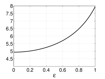
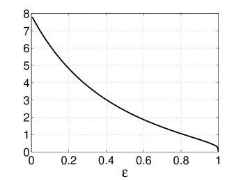
Figure 7: (a): $\frac{\epsilon^{2}/(1+\epsilon)}{\log\left(\cos\left(\frac{2\epsilon}{\pi}\right)\right)+\frac{4\epsilon}{\pi^{2}}\log(1+\epsilon)}$ as a function of $\epsilon$. (b): $\frac{\epsilon^{2}/(1+\epsilon)}{\log\left(\cos\frac{2\epsilon}{\pi}\right)-\frac{4\epsilon}{\pi^{2}}\log(1-\epsilon)+\frac{8}{3}\log\left(\cos\frac{\epsilon}{3\pi}\right)}$ as a function of $\epsilon$. Graphically, we know that it suffices to use a constant 8 in (110) and (116). The optimal constant will be different for different $\epsilon$. For example, if $\epsilon=0.2$, we could replace the constant 8 by a constant 5.

This completes the proof of Lemma 4.

E Proof of Lemma 6

Assume $x\sim C(0,d)$. The $\log$ likelihood ($l(x;d)$) and first three derivatives are

$$l(x;d)=\log(d)-\log(\pi)-\log(x^{2}+d^{2}),$$ (117)

$$l^{\prime}(d)=\frac{1}{d}-\frac{2d}{x^{2}+d^{2}}$$ (118)

$$l^{\prime\prime}(d)=-\frac{1}{d^{2}}-\frac{2x^{2}-2d^{2}}{(x^{2}+d^{2})^{2}}$$ (119)

$$l^{\prime\prime\prime}(d)=\frac{2}{d^{3}}+\frac{4d}{(x^{2}+d^{2})^{2}}+\frac{8d(x^{2}-d^{2})}{(x^{2}+d^{2})^{3}}$$ (120)

The MLE $\hat{d}_{MLE}$ is asymptotically normal with mean $d$ and variance $\frac{1}{k\text{I}(d)}$, where $\text{I}(d)$, the expected Fisher Information, is

$$\text{I}=\text{I}(d)=\text{E}\left(-l^{\prime\prime}(d)\right)=\frac{1}{d^{2}}+2\text{E}\left(\frac{x^{2}-d^{2}}{(x^{2}+d^{2})^{2}}\right)=\frac{1}{2d^{2}},$$ (121)

because

$$\text{E}\left(\frac{x^{2}-d^{2}}{(x^{2}+d^{2})^{2}}\right) =\frac{d}{\pi}\int_{-\infty}^{\infty}\frac{x^{2}-d^{2}}{(x^{2}+d^{2})^{3}}dx$$

$$=\frac{d}{\pi}\int_{-\pi/2}^{\pi/2}\frac{d^{2}(\tan^{2}(t)-1)}{d^{6}/\cos^{6}(t)}\frac{d}{\cos^{2}(t)}dt$$

$$=\frac{1}{d^{2}\pi}\int_{-\pi/2}^{\pi/2}\cos^{2}(t)-2\cos^{4}(t)dt$$

$$=\frac{1}{d^{2}\pi}\left(\frac{\pi}{2}-2\frac{3}{8}\pi\right)=-\frac{1}{4d^{2}}$$ (122)

Therefore, we obtain

$$\text{Var}\left(\hat{d}_{MLE}\right)=\frac{2d^{2}}{k}+O\left(\frac{1}{k^{2}}\right).$$ (123)

General formulas for the bias and higher moments of the MLE are available in (Bartlett, 1953; Shenton and Bowman, 1963). We need to evaluate the expressions in (Shenton and Bowman, 1963, 16a-16d), involving tedious algebra:

$$\text{E}\left(\hat{d}_{MLE}\right)=d-\frac{[12]}{2k\text{I}^{2}}+O\left(\frac{1}{k^{2}}\right)$$ (124)

$$\text{Var}\left(\hat{d}_{MLE}\right)=\frac{1}{k\text{I}}+\frac{1}{k^{2}}\left(-\frac{1}{\text{I}}+\frac{[1^{4}]-[1^{2}2]-[13]}{\text{I}^{3}}+\frac{3.5[12]^{2}-[1^{3}]^{2}}{\text{I}^{4}}\right)+O\left(\frac{1}{k^{3}}\right)$$ (125)

$$\text{E}\left(\hat{d}_{MLE}-\text{E}\left(\hat{d}_{MLE}\right)\right)^{3}=\frac{[1^{3}]-3[12]}{k^{2}\text{I}^{2}}+O\left(\frac{1}{k^{3}}\right)$$ (126)

$$\text{E}\left(\hat{d}_{MLE}-\text{E}\left(\hat{d}_{MLE}\right)\right)^{4}=\frac{3}{k^{2}\text{I}^{2}}+\frac{1}{k^{3}}\left(-\frac{9}{\text{I}^{2}}+\frac{7[1^{4}]-6[1^{2}2]-10[13]}{\text{I}^{4}}\right)$$

$$\hskip 122.85876pt+\frac{1}{k^{3}}\left(\frac{-6[1^{3}]^{2}-12[1^{3}][12]+45[12]^{2}}{\text{I}^{5}}\right)+O\left(\frac{1}{k^{4}}\right),$$ (127)

where, after re-formatting,

$$[12]=\text{E}(l^{\prime})^{3}+\text{E}(l^{\prime}l^{\prime\prime}),\hskip 21.68121pt[1^{4}]=\text{E}(l^{\prime})^{4},\hskip 21.68121pt[1^{2}2]=\text{E}(l^{\prime\prime}(l^{\prime})^{2})+\text{E}(l^{\prime})^{4},$$

$$[13]=\text{E}(l^{\prime})^{4}+3\text{E}(l^{\prime\prime}(l^{\prime})^{2})+\text{E}(l^{\prime}l^{\prime\prime\prime}),\hskip 21.68121pt[1^{3}]=\text{E}(l^{\prime})^{3}.$$ (128)

We will neglect most of the algebra. To help readers verifying the results, the following formula we derive may be useful:

$$\text{E}\left(\frac{1}{x^{2}+d^{2}}\right)^{m}=\frac{1\times 3\times 5\times...\times(2m-1)}{2\times 4\times 6\times...\times(2m)}\frac{1}{d^{2m}},\hskip 14.45377ptm=1,2,3,...$$ (129)

Without giving the detail, we report

$$\text{E}\left(l^{\prime}\right)^{3}=0,\hskip 21.68121pt\text{E}\left(l^{\prime}l^{\prime\prime}\right)=-\frac{1}{2}\frac{1}{d^{3}},\hskip 21.68121pt\text{E}\left(l^{\prime}\right)^{4}=\frac{3}{8}\frac{1}{d^{4}},$$

$$\text{E}(l^{\prime\prime}(l^{\prime})^{2})=-\frac{1}{8}\frac{1}{d^{4}},\hskip 21.68121pt\text{E}\left(l^{\prime}l^{\prime\prime\prime}\right)=\frac{3}{4}\frac{1}{d^{4}}.$$ (130)

Hence

$$[12]=-\frac{1}{2}\frac{1}{d^{3}},\hskip 18.06749pt[1^{4}]=\frac{3}{8}\frac{1}{d^{4}},\hskip 18.06749pt[1^{2}2]=\frac{1}{4}\frac{1}{d^{4}},\hskip 18.06749pt[13]=\frac{3}{4}\frac{1}{d^{4}},\hskip 18.06749pt[1^{3}]=0.$$ (131)

Thus, we obtain

$$\text{E}\left(\hat{d}_{MLE}\right)=d+\frac{d}{k}+O\left(\frac{1}{k^{2}}\right)$$ (132)

$$\text{Var}\left(\hat{d}_{MLE}\right)=\frac{2d^{2}}{k}+\frac{7d^{2}}{k^{2}}+O\left(\frac{1}{k^{3}}\right)$$ (133)

$$\text{E}\left(\hat{d}_{MLE}-\text{E}\left(\hat{d}_{MLE}\right)\right)^{3}=\frac{12d^{3}}{k^{2}}+O\left(\frac{1}{k^{3}}\right)$$ (134)

$$\text{E}\left(\hat{d}_{MLE}-\text{E}\left(\hat{d}_{MLE}\right)\right)^{4}=\frac{12d^{4}}{k^{2}}+\frac{222d^{4}}{k^{3}}+O\left(\frac{1}{k^{4}}\right).$$ (135)

Because $\hat{d}_{MLE}$ has $O\left(\frac{1}{k}\right)$ bias, we recommend the bias-corrected estimator

$$\hat{d}_{MLE,c}=\hat{d}_{MLE}\left(1-\frac{1}{k}\right),$$ (136)

whose first four moments are

$$\text{E}\left(\hat{d}_{MLE,c}\right)=d+O\left(\frac{1}{k^{2}}\right)$$ (137)

$$\text{Var}\left(\hat{d}_{MLE,c}\right)=\frac{2d^{2}}{k}+\frac{3d^{2}}{k^{2}}+O\left(\frac{1}{k^{3}}\right)$$ (138)

$$\text{E}\left(\hat{d}_{MLE,c}-\text{E}\left(\hat{d}_{MLE,c}\right)\right)^{3}=\frac{12d^{3}}{k^{2}}+O\left(\frac{1}{k^{3}}\right)$$ (139)

$$\text{E}\left(\hat{d}_{MLE,c}-\text{E}\left(\hat{d}_{MLE,c}\right)\right)^{4}=\frac{12d^{4}}{k^{2}}+\frac{186d^{4}}{k^{3}}+O\left(\frac{1}{k^{4}}\right),$$ (140)

by brute-force algebra. First, it is obvious that

$$\text{E}\left(\hat{d}_{MLE}-d\right)^{2}=\frac{2d^{2}}{k}+\frac{8d^{2}}{k^{2}}+O\left(\frac{1}{k^{3}}\right).$$ (141)

Then

$$\text{Var}\left(\hat{d}_{MLE,c}\right) =\text{E}\left(\hat{d}_{MLE,c}-\text{E}(\hat{d}_{MLE,c})\right)^{2}$$

$$=\text{E}\left(\hat{d}_{MLE}\left(1-\frac{1}{k}\right)-d+O\left(\frac{1}{k^{2}}\right)\right)^{2}$$

$$=\text{E}\left(\left(\hat{d}_{MLE}-d\right)\left(1-\frac{1}{k}\right)-\frac{d}{k}+O\left(\frac{1}{k^{2}}\right)\right)^{2}$$

$$=\text{E}\left(\hat{d}_{MLE}-d\right)^{2}\left(1-\frac{2}{k}\right)+\frac{d^{2}}{k^{2}}-2\frac{d}{k}\left(1-\frac{1}{k}\right)+O\left(\frac{1}{k^{3}}\right)$$

$$=\frac{2d^{2}}{k}+\frac{3d^{2}}{k^{2}}+O\left(\frac{1}{k^{3}}\right).$$ (142)

We can evaluate the higher central moments of $\hat{d}_{MLE,c}$ similarly, but we skip the algebra.

Therefore, we have completed the proof for Lemma 6.

References

- Achlioptas (2003) Dimitris Achlioptas. Database-friendly random projections: Johnson-Lindenstrauss with binary coins. Journal of Computer and System Sciences, 66(4):671–687, 2003.
- Aggarwal and Wolf (1999) Charu C. Aggarwal and Joel L. Wolf. A new method for similarity indexing of market basket data. In Proc. of SIGMOD, pages 407–418, Philadelphia, PA, 1999.
- Ailon and Chazelle (2006) Nir Ailon and Bernard Chazelle. Approximate nearest neighbors and the fast Johnson-Lindenstrauss transform. In Proc. of STOC, pages 557–563, Seattle, WA, 2006.
- Antle and Bain (1969) Charles Antle and Lee Bain. A property of maximum likelihood estimators of location and scale parameters. SIAM Review, 11(2):251–253, 1969.
- Arriaga and Vempala (1999) Rosa Arriaga and Santosh Vempala. An algorithmic theory of learning: Robust concepts and random projection. In Proc. of FOCS, pages 616–623, New York, 1999.
- Arriaga and Vempala (2006) Rosa Arriaga and Santosh Vempala. An algorithmic theory of learning: Robust concepts and random projection. Machine Learning, 63(2):161–182, 2006.
- Barnett (1966) V. D. Barnett. Evaluation of the maximum-likelihood estimator where the likelihood equation has multiple roots. Biometrika, 53(1/2):151–165, 1966.
- Bartlett (1953) M. S. Bartlett. Approximate confidence intervals, II. Biometrika, 40(3/4):306–317, 1953.
- Bhattacharya and Ghosh (1978) R. N. Bhattacharya and J. K. Ghosh. On the validity of the formal Edgeworth expansion. The Annals of Statistics, 6(2):434–451, 1978.
- Brinkman and Charikar (2003) Bo Brinkman and Mose Charikar. On the impossibility of dimension reduction in . In Proc. of FOCS, pages 514–523, Cambridge, MA, 2003.
- Brinkman and Charikar (2005) Bo Brinkman and Mose Charikar. On the impossibility of dimension reduction in . Journal of ACM, 52(2):766–788, 2005.
- Chapelle et al. (1999) Olivier Chapelle, Patrick Haffner, and Vladimir N. Vapnik. Support vector machines for histogram-based image classification. IEEE Trans. Neural Networks, 10(5):1055–1064, 1999.
- Chernoff (1952) Herman Chernoff. A measure of asymptotic efficiency for tests of a hypothesis based on the sum of observations. The Annals of Mathematical Statistics, 23(4):493–507, 1952.
- Chhikara and Folks (1989) Raj S. Chhikara and J. Leroy Folks. The Inverse Gaussian Distribution: Theory, Methodology, and Applications. Marcel Dekker, Inc, New York, 1989.
- Cysneiros et al. (2001) Francisco Jose De. A. Cysneiros, Sylvio Jose P. dos Santos, and Gass M. Cordeiro. Skewness and kurtosis for maximum likelihood estimator in one-parameter exponential family models. Brazilian Journal of Probability and Statistics, 15(1):85–105, 2001.
- Dasgupta and Gupta (2003) Sanjoy Dasgupta and Anupam Gupta. An elementary proof of a theorem of Johnson and Lindenstrauss. Random Structures and Algorithms, 22(1):60 – 65, 2003.
- Dhillon and Modha (2001) Inderjit S. Dhillon and Dharmendra S. Modha. Concept decompositions for large sparse text data using clustering. Machine Learning, 42(1-2):143–175, 2001.
- Efron et al. (2004) Bradley Efron, Trevor Hastie, Iain Johnstone, and Robert Tibshirani. Least angle regression. The Annals of Statistics, 32(2):407–499, 2004.
- Fama and Roll (1968) Eugene F. Fama and Richard Roll. Some properties of symmetric stable distributions. Journal of the American Statistical Association, 63(323):817–836, 1968.
- Fama and Roll (1971) Eugene F. Fama and Richard Roll. Parameter estimates for symmetric stable distributions. Journal of the American Statistical Association, 66(334):331–338, 1971.
- Feller (1971) William Feller. An Introduction to Probability Theory and Its Applications (Volume II). John Wiley & Sons, New York, NY, second edition, 1971.
- Ferecatu et al. (2004) Marin Ferecatu, Michel Crucianu, and Nozha Boujemaa. Retrieval of difficult image classes using SVD-based relevance feedback. In Prof. of Multimedia Information Retrieval, pages 23–30, New York, NY, 2004.
- Ferrari et al. (1996) Silvia L. P. Ferrari, Denise A. Botter, Gauss M. Cordeiro, and Francisco Cribari-Neto. Second and third order bias reduction for one-parameter family models. Stat. and Prob. Letters, 30:339–345, 1996.
- Fisher (1934) R. A. Fisher. Two new properties of mathematical likelihood. Proceedings of the Royal Society of London, 144(852):285–307, 1934.
- Frankl and Maehara (1987) P. Frankl and H. Maehara. The Johnson-Lindenstrauss lemma and the sphericity of some graphs. Journal of Combinatorial Theory A, 44(3):355–362, 1987.
- Gerber (1991) Hans U. Gerber. From the generalized gamma to the generalized negative binomial distribution. Insurance:Mathematics and Economics, 10(4):303–309, 1991.
- Gradshteyn and Ryzhik (1994) I. S. Gradshteyn and I. M. Ryzhik. Table of Integrals, Series, and Products. Academic Press, New York, fifth edition, 1994.
- Haas et al. (1970) Gerald Haas, Lee Bain, and Charles Antle. Inferences for the Cauchy distribution based on maximum likelihood estimation. Biometrika, 57(2):403–408, 1970.
- Hinkley (1978) David V. Hinkley. Likelihood inference about location and scale parameters. Biometrika, 65(2):253–261, 1978.
- Hougaard (1986) P. Hougaard. Survival models for heterogeneous populations derived from stable distributions. Biometrika, 73(2):387–396, 1986.
- Indyk (2000) Piotr Indyk. Stable distributions, pseudorandom generators, embeddings and data stream computation. In FOCS, pages 189–197, Redondo Beach,CA, 2000.
- Indyk (2001) Piotr Indyk. Algorithmic applications of low-distortion geometric embeddings. In Proc. of FOCS, pages 10–33, Las Vegas, NV, 2001.
- Indyk and Motwani (1998) Piotr Indyk and Rajeev Motwani. Approximate nearest neighbors: Towards removing the curse of dimensionality. In Proc. of STOC, pages 604–613, Dallas, TX, 1998.
- Indyk and Naor (2006) Piotr Indyk and Assaf Naor. Nearest neighbor preserving embeddings. ACM Transactions on Algorithms (to appear), 2006.
- Jensen (1995) Jens Ledet Jensen. Saddlepoint approximations. Oxford University Press, New York, 1995.
- Johnson and Lindenstrauss (1984) W. B. Johnson and J. Lindenstrauss. Extensions of Lipschitz mapping into Hilbert space. Contemporary Mathematics, 26:189–206, 1984.
- Lawless (1972) J. F. Lawless. Conditional confidence interval procedures for the location and scale parameters of the Cauchy and logistic distributions. Biometrika, 59(2):377–386, 1972.
- Lee and Naor (2004) James R. Lee and Assaf Naor. Embedding the diamond graph in and dimension reduction in . Geometric And Functional Analysis, 14(4):745–747, 2004.
- Li and Church (2005) Ping Li and Kenneth W. Church. Using sketches to estimate two-way and multi-way associations. Technical Report TR-2005-115, Microsoft Research, (A shorter version is available at www.stanford.edu/∼pingli98/publications/Report_Sketch.pdf), Redmond, WA, September 2005.
- Li et al. (2006a) Ping Li, Kenneth W. Church, and Trevor J. Hastie. Conditional random sampling: A sketched-based sampling technique for sparse data. Technical report, Department of Statistics, Stanford University (www.stanford.edu/~pingli98/publications/CRS_tr.pdf), 2006a.
- Li et al. (2006b) Ping Li, Trevor J. Hastie, and Kenneth W. Church. Improving random projections using marginal information. In Proc. of COLT, Pittsburgh, PA, 2006b.
- Li et al. (2006c) Ping Li, Trevor J. Hastie, and Kenneth W. Church. Sub-Gaussian random projections. Technical report, Department of Statistics, Stanford University (www.stanford.edu/~pingli98/report/subg_rp.pdf), 2006c.
- Li et al. (2006d) Ping Li, Trevor J. Hastie, and Kenneth W. Church. Very sparse random projections. In Proc. of KDD, Philadelphia, PA, 2006d.
- Li et al. (2006e) Ping Li, Debashis Paul, Ravi Narasimhan, and John Cioffi. On the distribution of SINR for the MMSE MIMO receiver and performance analysis. IEEE Trans. Inform. Theory, 52(1):271–286, 2006e.
- Lugosi (2004) Gabor Lugosi. Concentration-of-measure inequalities. Lecture Notes, 2004.
- McCulloch (1986) J. Huston McCulloch. Simple consistent estimators of stable distribution parameters. Communications on Statistics-Simulation, 15(4):1109–1136, 1986.
- Philips and Nelson (1995) Thomas K. Philips and Randolph Nelson. The moment bound is tighter than Chernoff’s bound for positive tail probabilities. The American Statistician, 49(2):175–178, 1995.
- Seshadri (1993) V. Seshadri. The Inverse Gaussian Distribution: A Case Study in Exponential Families. Oxford University Press Inc., New York, 1993.
- Severini (2000) Thomas A. Severini. Likelihood Methods in Statistics. Oxford University Press, New York, 2000.
- Shakhnarovich et al. (2005) Gregory Shakhnarovich, Trevor Darrell, and Piotr Indyk, editors. Nearest-Neighbor Methods in Learning and Vision, Theory and Practice. The MIT Press, Cambridge, MA, 2005.
- Shao (2003) Jun Shao. Mathematical Statistics. Springer, New York, NY, second edition, 2003.
- Shenton and Bowman (1963) L. R. Shenton and K. Bowman. Higher moments of a maximum-likelihood estimate. Journal of Royal Statistical Society B, 25(2):305–317, 1963.
- Strehl and Ghosh (2000) Alexander Strehl and Joydeep Ghosh. A scalable approach to balanced, high-dimensional clustering of market-baskets. In Proc. of HiPC, pages 525–536, Bangalore, India, 2000.
- Tibshirani (1996) Robert Tibshirani. Regression shrinkage and selection via the lasso. Journal of Royal Statistical Society B, 58(1):267–288, 1996.
- Tweedie (1957a) M. C. K. Tweedie. Statistical properties of inverse Gaussian distributions. I. The Annals of Mathematical Statistics, 28(2):362–377, 1957a.
- Tweedie (1957b) M. C. K. Tweedie. Statistical properties of inverse Gaussian distributions. II. The Annals of Mathematical Statistics, 28(3):696–705, 1957b.
- Vempala (2004) Santosh Vempala. The Random Projection Method. American Mathematical Society, Providence, RI, 2004.
- Zhu et al. (2003) Ji Zhu, Saharon Rosset, Trevor Hastie, and Robert Tibshirani. 1-norm support vector machines. In NIPS, 2003.
- Zolotarev (1986) V. M. Zolotarev. One-dimensional Stable Distributions. American Mathematical Society, Providence, RI, 1986.