Anytime coding on the infinite bandwidth AWGN channel:
A sequential semi-orthogonal optimal code

Abstract

It is well known that orthogonal coding can be used to approach the Shannon capacity of the power-constrained AWGN channel without a bandwidth constraint. This correspondence describes a semi-orthogonal variation of pulse position modulation that is sequential in nature — bits can be “streamed across” without having to buffer up blocks of bits at the transmitter. ML decoding results in an exponentially small probability of error as a function of tolerated receiver delay and thus eventually a zero probability of error on every transmitted bit. In the high-rate regime, a matching upper bound is given on the delay error exponent. We close with some comments on the case with feedback and the connections to the capacity per unit cost problem.

I Introduction

Shannon’s capacity theorem is arguably the greatest accomplishment in communications theory. Unfortunately, the random coding proof is non-constructive in that does not give a construction for any explicit code. This has led to the proverb: “Almost all codes are ”good” codes except for the the ones that we can think of.”[1] However, there is a channel for which explicit non-random constructions for capacity-achieving codes exist: the continuous-time AWGN channel with an input power constraint and no bandwidth constraint. (See, e.g. [2]) For such channels, it is further known that orthogonal signaling can be used to achieve data rates arbitrarily close to capacity. Orthogonality of the codewords plays the role of codeword independence in the discrete case. Recently, Liu and Viswanath have shown in [3] how to extend orthogonal coding to the “writing on dirty paper” scenario while continuing to preserve the interference-free infinite bandwidth error exponents. This correspondence extends orthogonal coding in a different direction to deal with “streaming data.”

I-A Model and block-coding review

The noise process is modeled as white with intensity $\frac{N_{0}}{2}$. The capacity of the channel is most naturally expressed in terms of energy per bit and is given by:

$$E_{b}>N_{0}\ln 2$$ (1)

which means that reliable communication is possible if the normalized energy per-bit exceeds $\ln 2$. When viewed in terms of bits per unit time, it means that reliable communication requires:

$$R<C_{\infty}=\frac{P}{N_{0}}\log_{2}e$$ (2)

where $P$ represents the allowed power per unit time.

One orthogonal signaling scheme is pulse position modulation (PPM) as depicted in Figure 1. Suppose there are $M$ possible messages to distinguish during one time slot of duration $T$. To communicate message $0\leq m\leq M-1$, the transmitter sends out a burst of its allocated transmit power during the time slot $[\frac{m}{M}T,\frac{m+1}{M}T]$ and is silent during the rest of the time slots. Since the time-slots are disjoint, the waveforms $x_{m}(t)$ corresponding to different messages $m$ are necessarily orthogonal over the interval $[0,T]$.

Figure 1: Pulse position modulation illustrated in the block coding framework.

Another set of orthogonal waveforms, more suitable for channels with amplitude-limits at the input, is depicted in Figure 2. These are sinusoids of different frequencies. If there are only amplitude-constraints but no binding power constraints, then “bang-bang” versions (square-waves) can also give orthogonal waveforms that have maximal energy given the amplitude constraint.

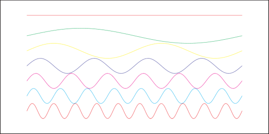
Figure 2: Another set of orthogonal waveforms: sinusoids of differing frequencies.

The receiver can do simple maximum-likelihood detection by having a bank of $M$ matched-filters that correlate the received signal $Y(t)$ with the $M$ orthogonal waveforms. The result of this correlation can be considered as $Z_{i}$ for message $i$ and due to the AWGN assumption, can be modeled as:

$$Z_{i}=\left\{\begin{array}[]{ll}N_{i}&\mbox{if }i\neq m\\ \sqrt{2E_{b}\log_{2}M}+N_{m}&\mbox{if }i=m\end{array}\right.$$ (3)

where the $N_{i}$ are iid standard zero-mean unit-variance Gaussian random variables, $E_{b}$ represents the normalized energy per bit, and $m$ represents the true message sent. $\log_{2}M$ represents the number of bits to be communicated.

In this case, ML decoding consists of finding the waveform with the highest $Z_{i}$. Classical analysis of this channel (see, e.g. [2]) shows that the orthogonal code with maximum-likelihood (ML) decoding has a probability of block error that goes to zero exponentially with block duration:

$$P_{e}\leq Ke^{-TE_{orth}(R)}$$ (4)

where $K$ is a rate dependent constant and

$$E_{orth}(R)=\left\{\begin{array}[]{rl}(\frac{C_{\infty}}{2}-R)\ln 2&\mbox{if }0\leq R\leq\frac{C_{\infty}}{4}\\ (\sqrt{C_{\infty}}-\sqrt{R})^{2}\ln 2&\mbox{if }\frac{C_{\infty}}{4}<R<C_{\infty}\\ 0&\mbox{otherwise}\end{array}\right.$$ (5)

Wyner showed in [4] that $E_{orth}(R)$ is also the best possible error exponent for this block-coding problem.

I-B Non-block coding

For a situation in which bits arrive from the source at regular intervals, the traditional view involves buffering up a block of $\log_{2}M$ bits, and then sending out the block of data using orthogonal signaling while waiting for the next block of data bits to arrive at the encoder. If there is only an energy constraint, then because there is no bandwidth constraint, the duration of signaling can be made as small as desired and hence essentially all the end-to-end delay can be attributed to the buffering at the encoder.

Figure 3: One block after another where each block uses an orthogonal code.

For DMCs and finite-bandwidth channels, convolutional codes and tree-codes provide an alternative to using block-codes. These codes have no buffering delay at the encoder and instead delay is incurred at the receiver. For DMCs, in principle random convolutional or tree codes eventually allow every bit to be decoded correctly, with a probability of error that converges to zero exponentially in delay at a rate given by the random coding error exponent [5]. Furthermore, at high rates for symmetric channels, it is known that no faster convergence is possible without feedback [6, 7].

There are also efficient decoding algorithms that work very well at low rates [8, 9] assuming oracle access to the code. Random convolutional codes can also be implemented using a computational cost that is linear in the constraint-length if the constraint is bounded, and linearly increasing with time if the constraint-length is infinite. If perfect tentative decision feedback is available, [7] also gives a scheme that gives infinite-constraint-length performance using only bounded expected computation per unit time.

To our knowledge, the infinite-bandwidth Gaussian counterparts to these ideas have not been developed in the literature. While clearly impractical, the codes in this paper have pedagogic value since they are explicit and so in many ways simpler than the random coding constructions for DMCs.

II The semi-orthogonal code

II-A Motivation: zero-rate coding by repetition

Consider a binary symmetric channel. The repetition code is an excellent code at zero-rate. To achieve a target reliability, just repeat a bit as many times as needed. To achieve perfect reliability, just repeat it infinitely often. Now, suppose that bits were arriving at the encoder regularly, but we neither cared about the delay in decoding them at the decoder nor about any increase in this delay with bit position. One strategy to communicate reliably would be as follows:

1. Initialize $i=1$

2. Output every bit $B_{1}^{i}$

3. Increment $i$

4. goto step 2.

This would result in an output stream $B_{1};B_{1},B_{2};B_{1},B_{2},B_{3};B_{1},B_{2},B_{3},B_{4};\ldots$ where the semicolons are used to denote the points of time at which we start repeating bits again and the commas mark off the channel uses. It is clear that if the decoder waits long enough, it will get enough repetitions of any individual bit to achieve its target reliability.

While this code has zero rate and has increasing required delay with time, it is possible to modify this scheme for use on the infinite bandwidth AWGN channel with finite rate, finite energy per bit, and fixed delays.

II-B Repeated/refined pulse position modulation

Suppose that bits are arriving every $\tau$ seconds and the encoder is allowed $E_{b}$ energy per bit. Rather than waiting to build up a buffer of $\log_{2}M$ bits and then signaling, suppose the encoder instead spent the $E_{b}$ energy immediately and used it to “repeat” the value of every bit received so far as in the scheme of Section II-A. The scheme is illustrated in Figure 4. It “refines” the information as time goes one.

Figure 4: Repeated pulse position modulation illustrated. The time slots are on the top and the possible sub-slots are on the bottom.

Lemma II.1

The repeated pulse position modulation code is semi-orthogonal.

If $x$ is the waveform corresponding to the bitstream $b$, and $x^{\prime}$ is the waveform corresponding to the bitstream $b^{\prime}$, then $x([(j-1)\tau,T]$ is orthogonal to $x^{\prime}([(j-1)\tau,T]$ whenever there exists a bit position $i\leq j$ for which $b_{i}\neq b^{\prime}_{i}$.

Proof: This is a simple consequence of the orthogonality of traditional pulse-position modulation. Since the underlying data bits differ somewhere at or before $j$, then over each time-slot after $(j-1)\tau$ the signals $x$ and $x^{\prime}$ have disjoint support. $\Box$

The time slot $[(k-1)\tau,k\tau]$ is divided into $2^{k}$ disjoint sub-slots and all the energy ($E_{b}$) is put into the sub-slot that corresponds to the realization of $B_{1}^{k}$ that has been seen so far at the encoder. If the target rate is $R=\frac{1}{\tau}$ and the target average power per unit time is $P$, then by using $E_{b}=\frac{P}{R}$, it is clear that this scheme meets the target power constraint — not just when we average over the realizations of the incoming bits $B$, but for every possible sequence of bits. Figure 5 illustrates the natural tree structure of this code.

Figure 5: The sub-slots in each time-slot are refinements of the sub-slots in the previous time-slot. This gives rise to a natural tree structure and the semi-orthogonality property of the code.

The decoder is assumed to have a target delay of $d\tau$ seconds and to be interested in estimating the value of the bits with that delay. In order to study asymptotic behavior, the interest is in the case of $d$ large but finite.

III Analysis of achievable $P_{e}$ with delay

Because this is a sequential encoding scheme that is going to be used with finite delay, the relevant error-event is a bit-error, not a block error. The goal is for the probability of bit-error to go to zero with delay. A code is considered to achieve reliability $E_{a}(R)$ if there exists a rate-dependent constant $K^{\prime}$ so that

$$P(\hat{B}_{i}\neq B_{i})\leq K^{\prime}e^{-d\tau E_{a}(R)}$$

for every $i>0,d>0$.

Our focus is on ML decoding. To get $\hat{B}_{i}$, the decoder has access to the received waveform $Y(t)$ over the interval $t\in[0,(i+d)\tau]$. Since no prior distribution over the $B_{i}$ is assumed, the following ML strategy is used:

• For every possible bit-sequence $\check{b}_{1}^{i+d}$, compute the log-likelihood $\ln p(Y([0,(i+d)\tau])=y([0,(i+d)\tau])|B_{1}^{i+d}=\check{b}_{1}^{i+d})$. By the white nature of the noise:

  $$\ln p(Y([0,(i+d)\tau])=y([0,(i+d)\tau])|B_{1}^{i+d}=\check{b}_{1}^{i+d})$$

  $$=\sum_{j=1}^{i+d}\ln p_{Y}(y([(j-1)\tau,j\tau])|B_{1}^{j}=\check{b}_{1}^{j})$$ (6)

• Pick the most likely sequence $\tilde{B}_{1}^{i+d}$ and emit its $i$-th position. In the white-Gaussian case, this will reduce to a picking the bit-sequence that results in the minimum Euclidean distance between waveforms.

It is important to note that the decisions are not remembered in this decoder. In principle, it recomputes the ML path each time.

III-A Suffix-error analysis

Suppose that a genie gave the decoder access to the correct value of the bits $B_{1}^{i-1}$. Since it knows the truth before time $(i-1)\tau$ and (• ‣ III) tells us that the log-likelihood is additive across time, the decoder only needs to consider $\ln p(Y([(i-1)\tau,(i+d)\tau])=y([(i-1)\tau,(i+d)\tau])|B_{1}^{i+d}=\check{b}_{1}^{i+d})$. The total duration of the relevant signal is thus $(d+1)\tau$.

The only way an error can occur is if one of the $2^{d}$ bitstreams with $\check{b}_{i}\neq b_{i}$ has a larger likelihood than the true stream. By Lemma II.1, the true waveform is orthogonal to all the false waveforms under consideration. Recalling that the block error probability analysis in Chap. 8 of [2] uses only the union bound and the fact that the true waveform is orthogonal to each of the false ones, we can immediately apply (4) to see that

$$P(\hat{B}_{i}\neq B_{i}\mbox{ at delay }d|B_{1}^{i-1}\mbox{ known})\leq Ke^{-(d+1)\tau E_{orth}(R)}$$ (7)

III-B Dealing with the uncertain prefix

The actual decoder does not know $B_{1}^{i-1}$. However, the error probability can be bounded as follows:

$$P(\hat{B}_{i}\neq B_{i}\mbox{ at delay }d)$$ (8)

$$\leq \sum_{j=0}^{i-1}P(\hat{B}_{i-j}\neq B_{i-j}\mbox{ at delay }d+j|B_{1}^{i-1-j}\mbox{ known})$$

since to make an error at bit $i$ the most likely sequence has to differ from the true sequence at $i$ or earlier. The regular union bound then gives us (8) with the earlier positions having correspondingly increased delays.

Combining (8) with (7) gives us:

$$P(\hat{B}_{i}\neq B_{i}\mbox{ with delay }d)$$

$$\leq \sum_{j=0}^{i-1}Ke^{-(d+1+j)\tau E_{orth}(R)}$$

$$< K(\sum_{j=0}^{\infty}e^{-(j+1)\tau E_{orth}(R)})e^{-d\tau E_{orth}(R)}$$

$$= \frac{K}{e^{\tau E_{orth}(R)}-1}e^{-d\tau E_{orth}(R)}$$

which gives the desired result with $E_{a}(R)=E_{orth}(R)$ and no dependence on either the bit position $i$ and delay $d$.

Theorem III.1

The repeated pulse position modulation code under maximum-likelihood decoding for individual bits with delay $d\tau$ achieves the orthogonal coding error exponent for every delay and bit position.

$$P(\hat{B}_{i}\neq B_{i}\mbox{ with delay }d)\leq K^{\prime}e^{-d\tau E_{orth}(R)}$$ (9)

An immediate consequence of theorem III.1 is that this code achieves zero probability of error on every bit in the limit of large delays. The limit here is purely at the decoder rather than being over encoder-decoder pairs. Consequently, it shows more clearly what the nature of reliable communication can be over the infinite-bandwidth channel. Using the language of anytime reliability [10, 11, 12], Theorem III.1 establishes a lower bound on the anytime reliability of the infinite-bandwidth AWGN channel without feedback.

The code as described is a pulse-position modulation variation that ends up requiring unboundedly large peak amplitudes while meeting a hard power constraint on the $\tau$ timescale. Because all that is required is orthogonality on each time slot, any other orthogonal signaling could be used. In particular, the code could use signals that have constant amplitude and just change abruptly in phase.

IV Upper bound on the error exponent with delay

In [6], Pinsker gave an derivation for the BSC showing that non-block codes without feedback could not beat the Sphere-Packing bound for how fast the probability of bit-error decays with end-to-end delay. This argument was given a more careful exposition and generalized to all DMCs without feedback in [7] with the Haroutunian bound [13] playing the role of the Sphere-Packing bound.

Here, we quickly show how to generalize Wyner’s block-coding converse result from [4] to the delay setting. Since Wyner’s argument was very block-specific (involving solid-angles, etc.), this is done by extending the argument of Section IV of [7] to the continuous-time AWGN case with a hard amplitude constraint. Let us examine the core steps of the proof from [7]:

1. Use a rate $R$ code with fixed-delay $d\tau$ to construct a hypothetical long block-code with rate $R-\delta$: this step is unchanged.

2. Consider “feedforward decoders” that have genie access to the truth about past bits. This step is also unchanged and so the error-event on a bit can be restricted to what the channel is like for the $d\tau$ time steps between when the bit entered the encoder and when its estimate emerges from the decoder.

3. Run the code over a “nearby” channel whose capacity is only sufficient to sustain a rate of $R-2\delta$. The data-processing inequality then forces the bit-error process to have an entropy rate of at least $\delta$. This step is unchanged in spirit, but the key here is not to consider a channel with increased noise but rather a channel that attenuates the input before adding the same noise as before. The attenuation factor $\sqrt{\frac{R-2\delta}{C_{\infty}}}$ chosen is such that the post-attenuation power can barely sustain a rate of $R-2\delta$ and thus cannot sustain $R-\delta$.

4. Fano’s inequality applied to the bit-error sequence reveals that the probability of bit-error under this channel’s induced probability measure is at least $\delta^{\prime}$. This step is also unchanged.

5. The feedforward nature of the decoder tells us that the error events only depend on the white noise realization for a duration of $d\tau$. This is also unchanged from [7]. Here, Wyner’s argument from [4] also enters and it is clear that since the decoder knows the true bits from the past, there are only $2^{d}$ possible waveforms that could have been transmitted. Expanding the white noise in the appropriately aligned basis means that only $2^{d}$ dimensions of noise are relevant. Without loss of generality, assume that one of these dimensions is exactly aligned with the waveform that was actually transmitted during this duration.

6. The probability of the error event has to be evaluated under the true channel law rather than the “nearby” law. Here, the story is considerably simpler than the DMC case. This is because the “nearby” channel behaves exactly the same as the original channel in the $2^{d}-1$ directions other than the true direction. Within the one true direction, typicality dictates that the nearby-channel noise is certainly going to be within $\pm Q^{-1}(\delta^{\prime})\sqrt{N_{0}}$ where $Q^{-1}$ just appropriately inverts the CDF for a standard Gaussian.

Thus, under the original channel law, the noise only has to push the $\sqrt{d\tau P}$ signal down to around:

$$\sqrt{d\tau P}(\sqrt{\frac{R-2\delta}{C_{\infty}}})\pm Q^{-1}(\delta^{\prime})\sqrt{N_{0}}$$

$$= \sqrt{\frac{d\tau P(R-2\delta)}{(P/N_{0})\log_{2}e}}\pm Q^{-1}(\delta^{\prime})\sqrt{N_{0}}$$

$$= \sqrt{\frac{d\tau(R-2\delta)N_{0}}{\log_{2}e}}\pm Q^{-1}(\delta^{\prime})\sqrt{N_{0}}$$

$$= \sqrt{N_{0}}(\sqrt{\frac{d\tau(R-2\delta)}{\log_{2}e}}\pm Q^{-1}(\delta^{\prime})$$

to cause an error. This means a noise for the original channel in this direction of around

$$-\sqrt{d\tau P}+\sqrt{N_{0}}(\sqrt{\frac{d\tau(R-2\delta)}{\log_{2}e}}\pm Q^{-1}(\delta^{\prime})$$

$$= -\sqrt{\frac{d\tau C_{\infty}N_{0}}{\log_{2}e}}+\sqrt{N_{0}}(\sqrt{\frac{d\tau(R-2\delta)}{\log_{2}e}}\pm Q^{-1}(\delta^{\prime})$$

$$= -\sqrt{d\tau N_{0}\ln 2}(\sqrt{C_{\infty}}-\sqrt{R-2\delta}\pm\frac{Q^{-1}(\delta^{\prime})}{d\tau\ln 2})$$

Thus the probability of error under the original channel law is at least

$$\frac{\delta^{\prime}}{2}\exp(-\frac{(\sqrt{d\tau N_{0}\ln 2}(\sqrt{C_{\infty}}-\sqrt{R-2\delta}+\frac{Q^{-1}(\delta^{\prime})}{d\tau\ln 2}))^{2}}{N_{0}}) = \frac{\delta^{\prime}}{2}\exp(-d\tau\ln 2(\sqrt{C_{\infty}}-\sqrt{R-2\delta}+\frac{Q^{-1}(\delta^{\prime})}{d\tau\ln 2})^{2}$$

Since $\frac{Q^{-1}(\delta^{\prime})}{d\tau\ln 2}$ is as small as desired when $d$ is large enough and $\delta,\delta^{\prime}$ were arbitrary, this essentially shows that the high rate expression for $E_{orth}(R)$ in (5) cannot be beaten with delay. Thus the semi-orthogonal code has essentially asymptotically optimal performance with delay.

V Interpretations and extensions

Is this a practical tool for data communication? It seems likely that the answer to this question is negative. Orthogonal signaling can be very wasteful of bandwidth and the semi-orthogonal scheme given here actually uses $\infty$ bandwidth which is never available in practice. The goal here is rather to refine our understanding of the role of delay in reliable communication and the tradeoffs possible between the encoder and decoder. It provides another extreme point balancing block-codes on the other side. Consequently, it is best to consider its theoretical rather than practical implications.

V-A Feedback

Without feedback, running an infinite-constraint-length random convolutional code would require performing an growing number of computations per unit time at the encoder just to generate the next channel input. Section II.C of [7] gives a way to use perfect tentative decision feedback to allow infinite-constraint-length convolutional codes to run using only bounded expected computation per time. Rather than convolving with the data from time zero till now to generate the channel inputs, the idea is to convolve against the current error sequence instead. The error sequence and the data bits are in one-to-one correspondence given knowledge of the current tentative estimates. Thus all the distance properties of the random infinite-constraint-length code are preserved along with all the expected probabilities of error. The encoding complexity is reduced dramatically since all bit-estimates from the distant past are almost always correct due to the exponential convergence of bit-estimates to true values.

In the infinite-bandwidth case here, this same trick can be used to reduce the bandwidth consumption in some similar “expected” sense. Consider the family of orthogonal waveforms from Figure 2. If both sine and cosine signals are used, then waveform $i$ has a frequency of about $\frac{i}{2\tau}$. Instead of transmitting a packet of energy $E_{b}$ that corresponds to all the bits sent so far, the packet can correspond to the current error-signal if the tentative decoder decisions are available at the transmitter. Once again, this does not change the semi-orthogonality property of the code because conditioned on the known tentative decisions, all suffixes in the codebook are still orthogonal to each other.

Figure 6: If tentative decision feedback is available, then ridiculously high frequencies are used only rarely as time goes on. Most of the time, the code will use low frequencies. The slope of the curve depends on the data rate: the higher the data rate, the more often high frequencies end up getting used.

Because of the exponential convergence of the probability of bit error, most of the early bits are correct and the errors are concentrated in the most recent bits. This gives rise to a bandwidth usage that is depicted in Figure 6. If the earliest current error is $d$ bits ago, then a frequency of at most $2^{\frac{d}{2}}$ needs to be used during this transmission. However the probability of that scales proportional to $2^{-E_{orth}(R)d}$. The two exponents fight each other to a power-law.

Note, while this seems to make the bandwidth requirements more reasonable, it does not make this a practical coding idea. The rolloff at high frequencies in traditional communication systems is not just a matter of not causing undue interference to users in adjacent bands. It is also about making the code itself robust to the behavior of users in those adjacent bands. Even when its transmissions are kept to low frequencies, the decoder remains very sensitive to the noise at all frequencies.

V-B Capacity per unit cost

Verdu’s capacity per unit cost framework [14] is the natural generalization of the infinite-bandwidth power-constrained AWGN channel. To see how the main result of this paper translates, the error calculation can be reinterpreted as a function of the number of bits intervening rather than in terms of the time delay and rate. Apply the substitutions $E_{b}=\frac{P}{R}$, $\tau=\frac{1}{R}$ to (2), (9), and (5) to get:

$$P(\hat{B}_{i}\neq B_{i}\mbox{ with }d\mbox{ bits intervening})\leq K^{\prime}e^{-dE_{orth}(\frac{E_{b}}{N_{0}})}$$ (10)

where $E_{orth}(\frac{E_{b}}{N_{0}})=$

$$\left\{\begin{array}[]{rl}(\frac{E_{b}}{N_{0}}(\frac{1}{2\ln 2})-1)\ln 2&\mbox{if }\frac{E_{b}}{N_{0}}>4\ln 2\\ (\sqrt{\frac{E_{b}}{N_{0}}(\frac{1}{\ln 2})}-1)^{2}\ln 2&\mbox{if }\ln 2<\frac{E_{b}}{N_{0}}\leq 4\ln 2\\ 0&\mbox{otherwise}\end{array}\right.$$ (11)

With this done, the infinite-bandwidth assumption can be dropped as long as the interest is only in the probability of error going to zero as a function of intervening energy. This gives rise to the natural “sequential” version of Verdu’s capacity per unit cost framework:

• There is a zero-cost channel input available.

• The encoder gets access to the bits one at a time and can use any number of channel uses it likes.

• The total cost of the channel uses so far must be less than $E_{b}$ times the number of bits the encoder has received.

• The decoder wants to estimate the values of all the bits, but is willing to wait until the encoder has spent a certain extra amount $dE_{b}$ more than it had when it first got access to the desired bit.

As the encoding strategy in [14] is a kind of pulse position modulation, the repeated pulse-position-modulation strategy described here translates directly into that framework. Interpret the sub-slots depicted in figure 4 as individual channel uses. The semi-orthogonality property of Lemma II.1 translates directly into a semi-disjoint support property. If the ML detector in the natural form is used, then (• ‣ III) continues to apply as appropriately interpreted. For error analysis analogous to (7), the ML performance can be bounded by the suboptimal, yet simple, hypothesis-testing based decoder in [14]. Since the error analysis in [14] relies only on the disjointness of the true codeword to each false one individually, all the arguments given here extend directly. All that is required for the prefix-argument of Section III-B to work is that the probability of error go to zero exponentially in $d$. Although this is not explicit in the stated proof in [14], it does indeed hold.

There is only one new consideration: integer effects. In the continuous amplitude situation, the transmitter could measure out any desired energy and pour it into a disjoint time period. For a DMC with an input cost constraint, there might be no way to hit the desired cost with a single input and so some way of time-sharing between inputs is essential.

It is here that we can see a role for a finite additional “delay” being imposed at the encoder. If the encoder decides to “burst” its output, it can do so by buffering up bits (spending no channel cost) until it has $L$ of them ready to go, and is willing to spend $LE_{b}$ cost to do the incremental encoding. By letting $L$ get large, $LE_{b}$ gets big enough to smooth out any integer constraint. However, the probability of error analysis given earlier continues to hold and the probability of $L$-burst error will go to zero exponentially at the correct rate with respect to cost increments.

In the capacity per unit cost formulation, this scheme or finitely truncated versions of it might actually have practical consequences. Consider a sensor network with very little energy available for long-range communication, but also very little data to send. If the data is going to be used by some application, the sensor may not know what the acceptable “delay” is. By using an anytime or delay-universal scheme like the one presented here, a sensor might be able to leave that choice to the decoder.

VI Conclusions and open problems

This correspondence shows how to communicate over the infinite-bandwidth AWGN channel in the non-block setting where bit-errors and end-to-end delays are important. An explicit semi-orthogonal coding scheme was developed and analyzed to show that the block-coding $E_{orth}(R)$ exponents are achievable with end-to-end delay. In the high-rate regime, a tight upper bound was given showing that the code is essentially optimal. While the basic semi-orthogonal coding strategy uses an increasing amount of bandwidth with time, if noiseless tentative decision feedback is available, the bandwidth usage can be made softer with high frequencies used only rarely.

The ideas here are taken only one-step toward the capacity-per-unit-cost formulation. It remains open to see what the optimal error exponents are with incremental cost and how to achieve them. In addition, the semi-orthogonal coding strategy for the capacity-per-unit-cost problem has a time-rate that tends to zero very rapidly as time advances. It is not clear if tricks similar to this paper can be used to combat this problem even if tentative decision feedback was available at the transmitter.

References

- [1] J. Wolf, “An introduction to turbo codes: The quintessential channel coding technique,” Tech. Rep., Mar. 2000.
- [2] R. G. Gallager, Information Theory and Reliable Communication. New York, NY: John Wiley, 1971.
- [3] T. Liu and P. Viswanath, “Opportunistic orthogonal writing on dirty paper,” IEEE Trans. Inform. Theory, vol. 52, no. 5, pp. 1828–1846, May 2006.
- [4] A. D. Wyner, “On the probability of error for communication in white Gaussian noise,” IEEE Trans. Inform. Theory, vol. 13, no. 1, pp. 86–90, Jan. 1967.
- [5] G. D. Forney, “Convolutional codes II. maximum-likelihood decoding,” Information and Control, vol. 25, no. 3, pp. 222–266, July 1974.
- [6] M. S. Pinsker, “Bounds on the probability and of the number of correctable errors for nonblock codes,” Problemy Peredachi Informatsii, vol. 3, no. 4, pp. 44–55, Oct./Dec. 1967.
- [7] A. Sahai, “Why block length and delay are not the same thing,” IEEE Trans. Inform. Theory, submitted. [Online]. Available: http://www.eecs.berkeley.edu/~sahai/Papers/FocusingBound.pdf
- [8] F. Jelinek, “Upper bounds on sequential decoding performance parameters,” IEEE Trans. Inform. Theory, vol. 20, no. 2, pp. 227–239, Mar. 1974.
- [9] G. D. Forney, “Convolutional codes III. sequential decoding,” Information and Control, vol. 25, no. 3, pp. 267–297, July 1974.
- [10] A. Sahai, “Any-time information theory,” Ph.D. dissertation, Massachusetts Institute of Technology, Cambridge, MA, 2001.
- [11] A. Sahai and S. K. Mitter, “The necessity and sufficiency of anytime capacity for stabilization of a linear system over a noisy communication link. part I: scalar systems,” IEEE Trans. Inform. Theory, vol. 52, no. 8, pp. 3369–3395, Aug. 2006.
- [12] ——, “Source coding and channel requirements for unstable processes,” IEEE Trans. Inform. Theory, Submitted, 2006. [Online]. Available: http://www.eecs.berkeley.edu/~sahai/Papers/anytime.pdf
- [13] E. A. Haroutunian, “Lower bound for error probability in channels with feedback,” Problemy Peredachi Informatsii, vol. 13, no. 2, pp. 36–44, 1977.
- [14] S. Verdú, “On channel capacity per unit cost,” IEEE Trans. Inform. Theory, vol. 36, no. 9, pp. 1019–1030, Sept. 1990.