The necessity and sufficiency of anytime capacity for stabilization of a linear system over a noisy communication link
Part II: vector systems

Abstract

In part I, we reviewed how Shannon’s classical notion of capacity is not sufficient to characterize a noisy communication channel if the channel is intended to be used as part of a feedback loop to stabilize an unstable scalar linear system. While classical capacity is not enough, a sense of capacity (parametrized by reliability) called “anytime capacity” is both necessary and sufficient for channel evaluation in this context. The rate required is the log of the open-loop system gain and the required reliability comes from the desired sense of stability. Sufficiency is maintained even in cases with noisy observations and without any explicit feedback between the observer and the controller. This established the asymptotic equivalence between scalar stabilization problems and delay-universal communication problems with feedback.

Here in part II, the vector-state generalizations are established and it is the magnitudes of the unstable eigenvalues that play an essential role. To deal with such systems, the concept of the anytime rate-region is introduced. This is the region of rates that the channel can support while still meeting potentially different anytime reliability targets for parallel message streams. All the scalar results generalize on an eigenvalue by eigenvalue basis. When there is no explicit feedback of the noisy channel outputs, the intrinsic delay of the unstable system tells us what the feedback delay needs to be while evaluating the anytime-rate-region for the channel. An example involving a binary erasure channel is used to illustrate how differentiated service is required in any separation-based control architecture.

I Introduction

One of Shannon’s key contributions was the idea that bits could be used as a single universal currency for communication. For a vast class of point-to-point applications, the communication aspect of the problem can be reduced to transporting bits reliably from one point to another where the required sense of reliability does not depend on the application. The classical source/channel separation theorems justify a layered communication architecture with an interface that focuses primarily on the message rate. Rate has the advantage of being additive in nature and so multiple applications can be supported over a single link by simple multiplexing of the message streams. This paradigm has been so successful in practice that researchers often assume that it is always valid.

Interactive applications pose a challenge to this separation based paradigm because long delays are costly. Part I of this paper [1] studies the requirements for the scalar version of the interactive application illustrated in Figure 1: stabilization of an unstable linear system with feedback that must go through a noisy communication channel. It turns out that message rate is not the only relevant parameter since the underlying noisy channel must also support enough anytime-reliability to meet the targeted sense of stability. However, the architectural implications of this result are unclear in the scalar case since there is only one message stream.

To better understand the architectural requirements for interactivity in a well defined mathematical setting, this correspondence considers the stabilization of linear systems with a vector-valued state. Prior work on communication-limited stabilization problems had also considered such vector problems from a source coding perspective. [2] showed that the minimum rate required is the sum of the logs of the magnitudes of the unstable eigenvalues and [3] extends the result to certain classes of unbounded driving disturbances. The multiparty case has begun to be addressed in the control community under the assumption of noiseless channels [4, 5]. The sequential rate-distortion bounds calculate the best possible control performance using a noisy channel that is perfectly matched to the unstable open-loop system while being restricted to having a specified Shannon capacity [6, 7]. Thus, the prior necessary conditions on stabilization are only in terms of Shannon capacity and the prior sufficient conditions required noiseless channels.

Figure 1: Control over a noisy communication channel. The unstable system is persistently disturbed by $\vec{W}_{t}$ and must be kept stable in closed-loop through the actions of ${\cal O,C}$.

The model of vector valued linear control systems is introduced in Section II and the main results are stated. Before going into the proofs, the significance of these results is demonstrated through an extended example in Section VI involving the stabilization of a vector-valued plant over a binary erasure channel. For this example, stabilization is impossible unless different bits are treated differently when it comes to transporting them across the noisy channel. These results establish that in interactive settings, a single “application” can fundamentally require different senses of reliability for its message streams. No single number can adequately summarize the channel and any layered architecture for reliable communication should allow applications to individually adjust the reliabilities on message streams. Recently, Pradhan has investigated block-coding reliability regions for distributed channel coding without feedback [8, 9]. This correspondence shows that reliability regions are interesting even in the point-to-point case in that they are both useful and nontrivial.

Section VI illustrates by example both the implications of the results as well as how to generalize the scalar results to vector systems with diagonalizable dynamics. The remaining ideas involved in proving the key results are given in Section VII for sufficiency and in Section VIII for necessity. Many aspects of the results here are straightforward generalizations from [1] using standard linear control theory tools. To avoid unnecessarily lengthening this correspondence, the details of these straightforward aspects are omitted. The reader familiar with [1, 10] should not have any difficulty in filling in the omitted details.

II The model and main results

The model is the same as in [1] except that everything is vector-valued. It is depicted in Figure 1. For convenience, all parts operate in discrete time with a common clock for stepping through time $t$.

The $n$-dimensional state of the control system at time $t$ is denoted $\vec{X}_{t}$ and evolves by

$$\vec{X}_{t+1}=A\vec{X}_{t}+B_{u}\vec{U}_{t}+B_{w}\vec{W}_{t},\ \ t\geq 0.$$ (1)

To be interesting, the matrix $A$ should have some unstable eigenvalues that lie strictly outside the unit circle. For the initial condition, depending on the context we assume either a known zero initial condition $\vec{X}_{0}=\vec{0}$ or a bounded initial condition $\|\vec{X}_{t}\|\leq\frac{\Omega_{0}}{2}$.

Any convenient finite-dimensional norm can be used since they are all equivalent. Consequently, this correspondence mostly assumes the $\infty-$norm $\|\vec{X}\|=\max_{i}|X(i)|$ for convenience. Throughout, subscripts are used to denote time indices, and the $i$-th component of of the vectors is selected using $X(i)$.

The noisy channel is a probabilistic system with an input and an output. At every time step $t$, it takes an input $a_{t}\in{\cal A}$ and produces an output $z_{t}\in{\cal Z}$ with probability $p(Z_{t}=z_{t}|a_{1}^{t},z_{1}^{t-1})$ where the notation $a_{1}^{t}$ is shorthand for the sequence $a_{1},a_{2},\ldots,a_{t}$. In general, the current channel output is allowed to depend on all inputs so far as well as on past outputs.

The $m_{y}$ dimensional input $\vec{Y}_{t}$ to the observer/encoder ${\cal O}$ is a linear function of the state corrupted by bounded additive noise.

$$\vec{Y}_{t}=C_{y}\vec{X}_{t}+\vec{N}_{t}.$$ (2)

The observer maps ${\cal O}_{t}:(I\!\!R^{m_{y}})^{t}\rightarrow{\cal A}$ take the observations $\vec{Y}_{1}^{t}$ and emit a channel input $a_{t}$.

The channel outputs $Z_{1}^{t}$ enter the controller maps ${\cal C}_{t}:{\cal Z}^{t}\rightarrow I\!\!R^{m_{u}}$ and result in the $m_{u}$-dimensional control signal $\vec{U}_{t}$.

The $\{\vec{W}_{t}\}$ is a bounded noise/disturbance sequence taking values in $I\!\!R^{m_{w}}$ s.t. $\|\vec{W}_{t}\|\leq\frac{\Omega}{2}$. Similarly, the observation noise $\{\vec{N}_{t}\}$ is only assumed to be bounded so that $\|\vec{N}_{t}\|\leq\frac{\Gamma}{2}$.

As in [1], the results in this correspondence impose no restrictions on the individual sequences $\{\vec{w}_{t}\},\{\vec{n}_{t}\}$ other than remaining bounded by $\Omega$ and $\Gamma$. In particular, no distribution is assumed for these disturbances. All distributions with bounded support are already covered by the sufficiency result here while the techniques of [11] can be applied to generalize the necessity result with suitable technical conditions.

All the randomness comes from the noisy channel and any randomization performed within the observer/encoder and controller/decoder. To be precise, the underlying sample space $\Omega_{\mbox{sample}}=\Omega_{\mbox{channel}}\times\Omega_{\mbox{code}}$. The channel’s randomness and the randomness available to the encoder/decoder are assumed to be independent of each other and this is reflected in the underlying sigma field ${\cal F}$ and probability map ${\cal P}$. However, once all the boxes in Figure 1 are connected together and the individual sequences $\{\vec{n}_{t}\},\{\vec{w}_{i}\}$ are specified, the $\{\vec{U}_{t},\vec{X}_{t},\vec{Y}_{t}\}$ become a well defined joint random process on the underlying probability space.

Definition III

(Parallels Definition 2.2 in [1]) A closed-loop dynamic system with state $\vec{X}_{t}$ is $\eta$-stable if there exists a constant $K$ s.t. for every $\{\vec{n}_{t}\},\{\vec{w}_{i}\}$ satisfying their bounds, the expectation $E[\|\vec{X}_{t}\|^{\eta}]\leq K$ for all $t\geq 0$.

The expectation is taken over all the randomness in the system, including the noisy channel and any randomness that the controller and observer can access. The constant $K$ may depend on the parameters of the system including the constants $\Omega,\Gamma$, but the bound on the $\eta$-th moment must hold for all times $t$ and uniformly over all individual sequences for both the driving disturbance and observation noise.

The equivalence of finite-dimensional norms guarantees that a bounded $\eta$-moment of the $\infty-$norm of $\vec{X}$ implies a bounded $\eta$-moment of any other norm and vice versa. This also implies that if the $\eta$-moment is bounded in one coordinate system it is also bounded in another coordinate system. Thus we will choose the coordinate system best matched to the system dynamics.

The goal is to design observers ${\cal O}_{t}$ and controllers ${\cal C}_{t}$ that $\eta$-stabilize the system.

III-A Dimensionality mismatches and intrinsic delay

Unlike the scalar case, the dimensions of $\vec{X},\vec{U},\vec{W},\vec{Y}$ can all be different. So even without a communication constraint, stabilizing the system in closed-loop requires $(A,C_{y})$ to be an observable pair. A pair of matrices $(A,C)$ is observable if the matrix $[C,CA,CA^{2},\ldots,CA^{n-1}]^{T}$ is of full rank [10]. This condition assures that by combining enough raw observations, all the modes of the linear dynamical system can be observed. The corresponding conditions on $(A,B_{u})$ and $(A,B_{w})$ is that they be reachable pairs. A pair of matrices $(A,B)$ is reachable if the matrix $[B,AB,A^{2}B,\ldots,A^{n-1}B]$ is of full rank [10]. This condition assures that by appropriate choice of inputs, all the modes of the linear dynamical system can be driven to a desired state.

Definition IV

The intrinsic delay $\Theta(A,B_{u},C_{y})$ of a linear system is the amount of time it takes the input to become visible at the output. It is the minimum integer $i\geq 0$ for which $C_{y}A^{i}B_{u}\neq 0$.

For single-input single-output (SISO) systems, this is just the position of the first nonzero entry in the impulse response.

IV-A Anytime capacity regions

Anytime capacity is introduced in [1] and related to traditional channel-coding reliability functions in [12]. In order to state the results for systems with vector-valued state, it is convenient to introduce the notion of an anytime rate region. Throughout this correspondence, rates $R$ are measured in units of bits per time step.

Definition V

A rate-tuple $(R_{1},R_{2},\ldots)$ sequential communication system over a noisy channel is a channel encoder ${\cal E}$ and channel decoder ${\cal D}$ pair such that:

• Messages $M_{i,t}$ enter the encoder at time $t$. Message $M_{i,t}=S_{i,\lfloor(t-1)R_{i}\rfloor+1}^{\lfloor tR_{i}\rfloor}$ corresponds to the $t$-th $R_{i}$-bit message sent in the $i$-th message stream and $M_{i,1}^{t-d}$ is shorthand for the sequence $(M_{i,1},M_{i,2},\ldots,M_{i,t-d})$. At the bit level, the $j$-th bit $S_{i,j}$ arrives at encoder $i$ at time $\frac{j}{R_{i}}$.

• The encoders ${\cal E}_{t}:{\cal Z}^{t-\theta}\times\{0,1\}^{\sum_{i=1}^{n}\lfloor R_{i}t\rfloor}\rightarrow{\cal A}$ with delay-$\theta$ feedback have access to past channel outputs $Z_{1}^{t-\theta}$ in addition to the message bits, and produce a channel input at times $t$ based on everything it has seen so far.

• The decoder ${\cal D}_{t}:{\cal Z}^{t}\rightarrow\{0,1\}^{\sum_{i=1}^{n}\lfloor R_{i}t\rfloor}$ produces updated estimates $\widehat{M}_{i,j}(t)$ for all $j\leq t$ based on all channel outputs observed till time $t$.

The anytime rate region ${\cal R}_{\mbox{any}}(\vec{\alpha})$ of a channel is the set of rate-tuples $(R_{1},R_{2},\ldots)$ that the channel can support using sequential communication. There has to exist a uniform constant $K$ so that for each $i$, all delays $d$, all times $t$, and all possible message sequences $\{M_{i,j}\}$,

$${\cal P}\left(\widehat{M}_{i,1}^{t-d}(t)\neq M_{i,1}^{t-d}(t)\right)<K2^{-\alpha_{i}d}.$$

No distribution is assumed for the bits $S_{i,j}$ and so this is essentially a requirement on the maximum probability of error. If common randomness is allowed, this is equivalent to assuming a uniform distribution over the bits and an average probability of error since the common randomness can be used to make the input look uniform by XORing each message bit with an iid fair coin toss known to both encoder and decoder.

The $\theta$-feedback anytime rate region refers to the rate region when noiseless channel output feedback is available to the encoder ${\cal E}$ with a delay of $\theta$ time units. If $\theta$ is omitted, it is to be understood as being one.

This generalizes the notion of a single feedback anytime capacity $C_{\mbox{any}}(\alpha)$ to a rate region ${\cal R}_{\mbox{any}}(\vec{\alpha})$ corresponding to a vector $\vec{\alpha}$ of anytime-reliabilities specifying how fast the probabilities of error tend to zero with delay for the different message streams.

Because all the message streams could simply be multiplexed together into a single stream in which everyone has the same reliability, it is obvious that ${\cal R}_{\mbox{any}}(\vec{\alpha})$ must contain the convex region defined by

$$R_{i} \geq 0,$$

$$\sum_{j}R_{j} < C_{\mbox{any}}(\max_{j}\alpha_{j}).$$ (3)

Similarly, if $\vec{R}^{\prime}\in{\cal R}_{\mbox{any}}(\vec{\alpha})$, then any rate vector obtained by stealing rate from higher reliability message streams and distributing it among lower reliability streams is also going to be within the rate region.

To get a simple outer bound, just notice that any single stream could be demultiplexed into parallel message streams and thereby achieve the anytime reliability of at least the minimum of the parallel anytime reliabilities. For convenience, assume that $\vec{\alpha}$ is sorted so that $\alpha_{1}\geq\alpha_{2}\geq\cdots\geq\alpha_{n}$. This means that ${\cal R}_{\mbox{any}}(\vec{\alpha})$ must be contained within the region defined by the intersection of the following regions:

$$R_{i} \geq 0$$

$$\sum_{j=1}^{k}R_{j} \leq C_{\mbox{any}}(\alpha_{k})$$ (4)

as $i,k$ range over all the message stream indices.

V-A Main results

Since the vector $\vec{\lambda}$ of unstable eigenvalues (if an eigenvalue has multiplicity, then it should appear in $\vec{\lambda}$ multiple times) plays an important role in these results, some shorthand notation is useful. $\vec{\lambda}_{||}$ is used to denote the component-wise magnitudes of the $\vec{\lambda}$. $\log_{2}(\vec{\lambda_{||}})$ is used to denote the component-wise logarithms of those magnitudes.

Theorem V.1

For some $\vec{\epsilon}>0$, assume a noisy finite-output-alphabet channel such that the $(\theta+1)$-feedback anytime rate region ${\cal R}_{\mbox{any}}(\eta\log_{2}\vec{\lambda}_{||}+\vec{\epsilon})$ contains the rate vector $(\log_{2}(\vec{\lambda_{||}})+\vec{\epsilon})$. Also assume an unknown initial condition $\vec{X}_{0}$ that is bounded $\|\vec{X}_{t}\|\leq\frac{\Omega_{0}}{2}$.

If the observer has access to the observations $\vec{Y}_{t}$ corrupted by bounded additive noise, then any linear system with dynamics described by (1) with unstable eigenvalues $\vec{\lambda}$, reachable $(A,B_{u})$, observable $(A,C_{y})$, intrinsic delay $\Theta(A,B_{u},C_{y})\leq\theta$ can be $\eta$-stabilized by constructing an observer ${\cal O}$ and controller ${\cal C}$ for the unstable vector system that together achieve $E[\|\vec{X}_{t}\|^{\eta}]<K$ for all sequences of bounded driving noise $\|\vec{W}_{t}\|\leq\frac{\Omega}{2}$ and all sequences of bounded observation noise $\|\vec{N}_{t}\|\leq\frac{\Gamma}{2}$.

If the observer maps ${\cal O}_{t}$ are also allowed direct access to the past channel outputs with delay $\theta^{\prime}\geq 1$, then it suffices to just consider the $\min(\theta^{\prime},\theta+1)$-feedback anytime rate region.

By applying (3) to Theorem V.1, one immediately gets the following easier to check corollary:

Corollary V.1

If the sum of the logarithms of the magnitudes of the unstable eigenvalues of a system matching the conditions of Theorem V.1 is less than the $(\theta+1)$-delayed feedback anytime capacity $C_{\mbox{any}}(\eta\max_{i}\log_{2}|\lambda_{i}|)$, then it is possible to $\eta$-stabilize the system over the noisy channel in the same sense as in Theorem V.1.

For the necessity direction, the requirements are relaxed and we only assume that a control system exists that works with a known $\vec{0}$ initial condition and without noise in the observations since these make the task of the observer and controller easier.

Theorem V.2

Assume that for a given noisy channel, system dynamics described by (1) with reachable $(A,B_{W})$, observable $(A,C_{y})$, zero initial condition $\vec{X}_{0}=\vec{0}$, eigenvalues $\vec{\lambda}$ and $\eta>0$, that there exists an observer ${\cal O}$ and controller ${\cal C}$ for the unstable vector system that achieves $E[\|\vec{X}_{t}\|^{\eta}]<K$ for all sequences of bounded driving noise $\|\vec{W}_{t}\|\leq\frac{\Omega}{2}$ and all $t$.

Let $|\lambda_{i}|>1$ for $i=1\ldots l$, and let $\vec{\lambda}$ be the $l$-dimensional vector consisting of only the exponentially unstable eigenvalues of $A$. Then for every $\vec{\epsilon_{1}},\vec{\epsilon_{2}}>0$ the rate vector $(\log_{2}\vec{\lambda}_{||}-\vec{\epsilon_{1}})$ is contained within the $(\Theta(A,B_{u},C_{y})+1)$-feedback anytime rate region ${\cal R}_{\mbox{any}}(\eta\log_{2}\vec{\lambda}_{||}-\vec{\epsilon_{2}})$ for this same noisy channel.

This theorem reveals that each unstable eigenvalue, no matter whether it has its own eigenvector or not, induces a demand that the channel be able to reliably transport a message stream. The sufficient conditions of Theorem V.1 and the necessary conditions of Theorem V.2 match each other $\pm\vec{\epsilon}$.

VI Differentiated Service Example

This section studies a simple numeric example of a vector valued unstable plant. An explicit self-contained five-dimensional example was given in [13] for the binary erasure channel, but here a simpler two-dimensional example is given that leverages the results from [12].

$$A=\left[\begin{array}[]{cc}2^{0.34}&0\\ 0&2^{0.05}\end{array}\right]$$ (5)

where the observer has noiseless access to both the state $\vec{X}$ and the applied control signals $\vec{U}$. The controller can apply any $2$-dimensional input that it wishes. Assume that the disturbance $\vec{W}$ satisfies $\|\vec{W}_{t}\|_{\infty}\leq\frac{1}{2}$ for all times $t$. Thus, this example consists of two independent scalar systems that must share a single communication channel.

Section VI-A reviews how it is possible to hold this system’s state within a finite box over a noiseless channel using total rate $R=0.392$ consisting of one bitstream at rate $0.341$ and another bitstream of rate $0.051$. Section VI-B considers a particular binary erasure channel and shows that if it is used without distinguishing between the bitstreams, then third-moment stability cannot be achieved. Section VI-C shows how a simple priority based system can distinguish between the bitstreams and achieve third-moment stability while essentially using the observer/controller originally designed for the noiseless link. Finally, Section VI-D discusses how this diagonal example can be transformed into a single-input single-output control problem that suffers from the same limitations.

VI-A Design for a noiseless channel

The system defined by (5) consists of two independent scalar systems and so each of these falls under [1]. Since

$$0.341 > 0.34$$

$$0.051 > 0.05,$$

Theorem 4.1 in [1] guarantees that it is sufficient to use two parallel bitstreams of rates $R_{1}=0.341$ (for the first subsystem) and $R_{2}=0.051$ (for the second subsystem) to stabilize the system over a noiseless channel. The total rate is $0.392$ bits per channel use.

VI-B Treating all bits alike

A strict layering-oriented design attempts to use a virtual bit-pipe interface to connect the observers and controllers from the previous section. Consider a binary erasure channel with erasure probability $\beta=0.4$ and noiseless feedback available to the encoder. There is clearly enough Shannon capacity since $1-0.4=0.6>0.392$. To minimize latency, the natural choice of coding scheme is a single FIFO queue in which bits are retransmitted until they get through correctly. The system is illustrated in Figure 2.

Figure 2: Forcing all the bitstreams to get the same treatment for reliable communication

If a channel-code does not differentiate among the substreams, then the code would have to give the same anytime reliability to all the bits. The minimum anytime reliability required is $\alpha^{*}=3\log_{2}2^{0.34}=1.02$. For the binary erasure channel, there is exact expression for the feedback anytime-capacity:[12, Theorem 3.3]

$$C_{\mbox{any}}(\alpha)=\frac{\alpha}{\alpha+\log_{2}(\frac{1-\beta}{1-\beta 2^{\alpha}})}.$$ (6)

Plugging in $\beta=0.4$ and $\alpha=1.02$ into (6) reveals that the channel can only carry $\approx 0.38<0.39$ bits/channel-use with the required reliability. Thus, it is impossible to simultaneously attain the required rate/reliability pair by using a channel code that treats all message bits alike.

VI-C Differentiated service

The main difficulty encountered in the previous section is that the most challenging reliability requirement comes from the larger eigenvalue, while the total rate requirement involves both the eigenvalues. This section explores the idea of differentiated service at the reliable communication layer as illustrated in the simple priority-based scheme of Figure 3. This is used to give extra reliability (shorter delays) to the bitstream corresponding to the first subsystem at the expense of lower reliability (higher delays) for the second one.

• Place bits from the different streams into prioritized FIFO buffers.

• At every channel use, transmit the oldest bit from the highest priority input buffer that is not empty.

• If the bit is received correctly, remove it from the appropriate input buffer.

• If there are no bits waiting in any buffer, then send a dummy bit across the channel.

Two priority levels are used. The higher one corresponds to the rate $R_{1}=0.341$ bitstream coming from the first subsystem with eigenvalue $2^{0.34}$. The lower one corresponds to the rate $R_{2}=0.051$ bitstream and corresponds to the subsystem with eigenvalue $2^{0.05}$.

The decoder functions on a stream-by-stream basis. Since there is noiseless feedback and the encoder’s incoming bitstreams are deterministic in their timing, the decoder can keep track of the encoder’s buffer sizes. As a result, it knows which incoming bit belongs to which stream and can pass the received bit on to the appropriate subsystem’s controller. The sub-system controllers are patched as in the proof of Theorem 4.1 in [1] — they apply $\lambda_{i}^{d}U_{i}(t_{o})$ if their bit arrives with a delay of $d$ time-steps instead of showing up at time $t_{o}$ as expected.

Figure 3: The strict priority queuing strategy for discrimination between bitstreams. Lower priority buffers are served only if the higher priority ones are empty.

All that remains is to calculate a lower bound on the anytime reliabilities delivered by such a communication scheme.

Theorem VI.1

For the binary erasure channel with erasure probability $\beta>0$ used with the strict two-priority encoder above, high-priority rate $0<R_{H}<1-\beta$ and low-priority rate $0\leq R_{L}<1-\beta-R_{H}$, the system attains anytime-reliabilities $\alpha_{H},\alpha_{L}$ satisfying

$$\alpha_{H} = C_{\mbox{any}}^{-1}(R_{H})$$

$$\alpha_{L} \geq \max_{\rho\leq\rho_{HL}}E_{0}(\rho)-\rho R_{H}$$ (7)

where

$$E_{0}(\rho)=-\log_{2}(\beta+2^{-\rho}(1-\beta))$$ (8)

is the base-2 Gallager function for the BEC from [14] and $\rho_{HL}$ is the unique solution to

$$R_{H}+R_{L}=\frac{E_{0}(\rho_{HL})}{\rho_{HL}}.$$ (9)

When $R_{L}$ is low enough, the bound (7) evaluates to the sphere-packing bound $D(1-R_{H}||\beta)$ for the anytime reliability $\alpha_{L}$ of the lower-priority bitstream.

Proof: See Appendix A.

Numerical evaluation of the bound (7) for the rate-pair $R_{H}=R_{1}=0.341,R_{L}=R_{2}=0.051$ gives the anytime reliabilities $\alpha_{1}\approx 1.11>1.02$ and $\alpha_{2}\geq 0.196>0.15$. This reveals that the both subsystems will remain stable in the third-moment sense.

All of this is illustrated graphically in Figure 4. The diagonal lines have a slope of $\eta=3$. The marked $\times$ on the plot has rate equal to $0.34+0.05$ and a reliability of $3*0.34$. Since it is outside the anytime capacity region demarcated by the BEC’s uncertainty-focusing bound, it is not achievable. The two marked $\diamond$ points represent the reliabilities achieved by the high and low priority streams. Notice that both are above their corresponding diagonal lines and so the resulting closed-loop system is $3$-stable.

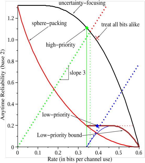
Figure 4: The anytime capacity curve for the binary erasure channel, along with the sphere-packing bound and an evaluation of the low-priority bound for $R_{H}=0.341$. The parabolic curve under the low-priority bound illustrates what happens as $\rho$ ranges in (7). The maximum of the curve is attained at the sphere-packing bound.

VI-D Interpreting the example

The diagonal system example given here is subject to two simple interpretations. First, it can be interpreted as two physically distinct control systems that must share a common bottleneck communication link. Thus, it represents an information-theoretic example of how different interactive applications sharing the same communication link can require differentiated service by the reliable communication layer even in the context of an asymptotic binary performance objective like $\eta$-stabilization.

Alternatively, this example can be packaged into a single system with a vector valued state. This vector-state valued system can even be at the heart of a SISO control system. Consider the change of coordinates matrix:

$$T=\left[\begin{array}[]{cc}1&-1\\ 0&1\end{array}\right]$$ (10)

This transformation is used to define $\widetilde{A}=TAT^{-1}$ using (10) and (5) results in

$$\widetilde{A}=\left[\begin{array}[]{cc}2^{0.34}&2^{0.05}-2^{0.34}\\ 0&2^{0.05}\end{array}\right].$$ (11)

The $B_{w}$ matrix remains the identity while

$$B_{u}=\left[\begin{array}[]{c}0\\ 1\\ \end{array}\right]$$ (12)

and

$$C_{y}=[1,1].$$ (13)

This is clearly an unstable SISO system with a scalar observation $Y_{t}$ and scalar control $U_{t}$. As a scalar system, it has two real poles at $2^{0.34}$ and $2^{0.05}$. Both are outside the unit circle.

It is easy to verify that $C_{y}$ and $C_{y}\widetilde{A}$ are linearly independent and thus the system is observable. If there were neither controls nor driving disturbances, then an observer ${\cal O}$ could take an appropriate linear combination of two consecutive scalar observations $Y_{i},Y_{i+1}$ to recover the state $\vec{X}_{i}$ exactly. Explicitly, $X_{i}(1)=\frac{(2^{0.34}-2^{1.05})Y_{i}+Y_{i+1}}{2^{1.34}-2^{1.05}}$ and $X_{i}(2)=\frac{2^{0.34}Y_{i}-Y_{i+1}}{2^{1.34}-2^{1.05}}$.

The driving disturbance shows up as an additional “noise” in $\vec{X}_{i+1}$. Hence the effective observation noise in $Y_{i}$ is $N_{i}$ and the effective observation noise in $Y_{i+1}$ is $W_{i}(1)+W_{i}(2)+N_{i+1}$. So the estimation error $|\widehat{X}_{i}(1)-X_{i}(1)|\leq\frac{(2^{1.05}-2^{0.34}+1)\Gamma+2\Omega}{2(2^{1.34}-2^{1.05})}$ and similarly $|\widehat{X}_{i}(2)-X_{i}(2)|\leq\frac{(2^{0.34}+1)\Gamma+2\Omega}{2(2^{1.34}-2^{1.05})}$. This can be interpreted as a larger $\Gamma^{\prime}$ that bounds the norm of the effective observation noise.

To support the estimation performed at the observer, the controller could either refrain from applying any controls for two consecutive time-instants or equivalently apply control signals that are perfectly known to the observer.

Similarly, the controllability conditions are satisfied since $B_{u}$ and $\widetilde{A}B_{u}$ are linearly independent. By identical reasoning, this means that the controller can apply any desired control to each of the underlying states by preparing scalar controls in batches of two consecutive time units. Thus, the controller can alternate between applying a zero control for two time units and then applying a batched control for the next two time units.

Stabilizing the output of the SISO system clearly requires stabilizing all of the internal states since the system is observable. Since the internal state evolution of this system is governed by $\widetilde{A}$, it is essentially the same as that governed by the diagonal $A$ since the two differ only by a linear change of coordinates. This means that differentiated service across the erasure channel is required for this single SISO system as well!

VII Sufficiency: Proof of Theorem V.1

Theorem V.1 is proven in stages. The scalar case is in [1] and as Section VI-D shows, the scalar results immediately generalize to systems with purely diagonal dynamics through a change of coordinates. The bounded initial condition can be interpreted as a zero initial condition and bounded driving noise, but for a system that starts at time $-1$. Consequently, the first new issue concerns systems with nondiagonal Jordan blocks. After that, we consider general systems that are reachable and observable, but where the anytime code is assumed to be a black-box with its own access to channel feedback. Finally, we show how to operate a feedback anytime code without any explicit feedback path for the channel outputs.

VII-A Non-diagonal Jordan blocks.

Proposition VII.1

For some $\vec{\epsilon}>0$, assume access to an anytime-code that supports the rate vector $(\log_{2}(\vec{\lambda_{||}})+\vec{\epsilon})$ with anytime reliabilities $\eta\log_{2}\vec{\lambda}_{||}+\vec{\epsilon}$.

Consider an $n$-dimensional linear system with dynamics described by (1) having positive real unstable eigenvalues $\vec{\lambda}$, $A$ in block-diagonal form with each block being upper-triangular and having a single real-valued eigenvalue $|\lambda|$ on its diagonal, $B_{u}$ and $C_{y}$ as identity matrices so that each state can be individually controlled, with observations $\vec{Y}_{t}$ corrupted by bounded additive noise.

Then for all $\Omega\geq 0,\Gamma\geq 0$, there exists a $K>0$ so that the system can be $\eta$-stabilized by constructing an observer ${\cal O}$ and controller ${\cal C}$ for the unstable vector system that together achieve $E[\|\vec{X}_{t}\|^{\eta}]<K$ for all sequences of bounded driving noise $\|\vec{W}_{t}\|\leq\frac{\Omega}{2}$ and all sequences of bounded observation noise $\|\vec{N}_{t}\|\leq\frac{\Gamma}{2}$.

Furthermore, this continues to hold even if the controller is restricted to applying a nonzero control signal only every $n$ time steps and the observer is similarly restricted to sample the state every $n$ time steps.

Proof: Because the blocks corresponding to different eigenvalues do not interact with each other in the specified model, it suffices to consider an $n$-dimensional square $A$ matrix that represents a single upper-triangular block.

$$A=\left[\begin{array}[]{ccccc}\lambda&a_{12}&a_{13}&\cdots&a_{1n}\\ 0&\lambda&a_{23}&\cdots&a_{2n}\\ \vdots&0&\ddots&\ddots&\\ 0&0&\cdots&\lambda&a_{n-1,n}\\ 0&0&\cdots&0&\lambda\end{array}\right]$$ (14)

There are two key observations. The first is that the dynamics for the last component $X_{t}(n)$ are the same as in the scalar case — $X_{t+1}(n)=\lambda X_{t}(n)+W_{t}(n)+U_{t}(n)$. This faces a driving disturbance with bound $\Omega_{n}=\Omega$.

The second is that the dynamics for all the other components are given by:

$$X_{t+1}(i)=\lambda X_{t}(i)+U_{t}(i)+W_{t}(i)+\sum_{j=i+1}^{n}a_{i,j}X_{t}(j)$$ (15)

Recall that the constructions in Section IV.B of [1] (duplicated here in Appendix C for reader convenience) are based on having a virtual controlled process $\bar{X}$ that is stabilized over a finite-rate noiseless channel in a manner that keeps the virtual state within a $\Delta$-sized box, no matter what the disturbances are. The observer essentially tells the controller what controls to apply so as to do this and protects these instructions with an anytime channel code.

Group together the weighted sum of the bounded virtual controlled state dimensions $\sum_{j=i+1}^{n}a_{i,j}\bar{X}_{t}(j)$ and the net disturbance $W_{t}(i))$ into a single disturbance term. The new bound on the disturbance is simply

$$\Omega_{i}=\Omega+\sum_{j=i+1}^{n}|a_{i,j}|\Delta_{j}$$

where $\Delta_{j}$ are computed recursively using the following formula from [1]:

$$\Delta_{j}=\frac{\Omega_{j}}{1-\lambda 2^{-R}}$$

where $R>\log_{2}\lambda$.

Since there are only a finite number of state dimensions, this shows that “in the box” stabilization is possible using noiseless channels at the appropriate rates. Just as in [1], if used with an anytime code, the control signal must take care to counteract the impact of any previously erroneous control signals. Let $\widetilde{X}_{t}$ represent the state at time $t$ that would result from only the actual controls applied (no disturbances) till time $t-1$. $A\widetilde{X}_{t}$ is the prediction for what that would evolve into if a zero control were to be applied at time $t$. The current message estimates from the anytime code at time $t$ reveal what the desired value for $\widetilde{X}_{t+1}$ is. As $B_{u}$ is the identity, the actual applied control signal is just the difference $\widetilde{X}_{t+1}-A\widetilde{X}_{t}$.

The only remaining question concerns the impact on state $j$ of such temporary anytime decoding errors on message stream $i>j$. Recall that the “impulse response” on state $j$ of an impulse on state $i$ at time $0$ is given by $p_{i,j}(t)\lambda^{t}$ where $p(t)$ is some polynomial in $t$ of order $i-j$ where the polynomial depends on the elements of the $A$ matrix. The polynomial is bounded above by $K(\lambda^{\epsilon})^{t}$ where $K$ is a constant depending on $A,n,\lambda,\epsilon$ and $\epsilon>0$ can be chosen as small as desired. $K$ can further be multiplied by the (small) constant $n$ to bound the net impact of an error on state $j$ from a decoding error in any combination of message streams $i>j$.

Since the message streams have anytime reliability $\alpha_{i}$ individually, they have anytime reliability $\min_{i}\alpha_{i}$ when considered together as a single stream. Since the relevant anytime reliability $\min_{i}\alpha_{i}>\eta\log_{2}\lambda$, we can choose $\epsilon$ so that $\alpha_{i}>\eta(1+\epsilon)\log_{2}\lambda$ as well. Thus, by the same arguments as Section IV.D of [1], all the $\eta$-moments in the block will be bounded.

Notice that $A^{n}$ is also upper-triangular with diagonal terms of $\lambda^{n}$. Thus, by arguments identical to those of Theorem 4.4 in [1], the results continue to hold if both the observer and controller are restricted to act only every $n$ time steps. $\Box$

VII-B Changing coordinates: complex unstable eigenvalues

The restriction to real block-diagonal upper-triangular systems in Proposition VII.1 is easily overcome by choosing the right coordinate frame.

Proposition VII.2

Proposition VII.1 holds even if the real $A$ matrix has complex unstable eigenvalues $\vec{\lambda}$.

Proof: To avoid any complications arising from the complex eigenvalues, the real Jordan normal form can be used [15]. This guarantees that there exists a nonsingular real matrix $V$ so that $VAV^{-1}$ is a diagonal sum of either traditional real-valued Jordan blocks corresponding to the real eigenvalues and special real-valued “rotating” Jordan blocks corresponding to each pair of complex-conjugate eigenvalues. The rotating block for the pair $\lambda=\lambda_{r}+\lambda_{j}\sqrt{-1}$ and its conjugate is a real two-by-two matrix:

$$\left[\begin{array}[]{cc}\lambda_{r}&\lambda_{j}\\ -\lambda_{j}&\lambda_{r}\end{array}\right]$$

$$= \left[\begin{array}[]{cc}|\lambda|&0\\ 0&|\lambda|\end{array}\right]\left[\begin{array}[]{cc}\cos(\angle\lambda)&\sin(\angle\lambda)\\ -\sin(\angle\lambda)&\cos(\angle\lambda)\end{array}\right]$$

which is clearly a product of a scaling matrix and a rotation matrix. Group these two-by-two rotating blocks into a block-diagonal unitary matrix $R$. So $VAV^{-1}=\Lambda R$ where $\Lambda$ is now a real block-diagonal matrix whose constituent blocks are upper-triangular and whose diagonals consist of the magnitudes of the eigenvalues.

The key is to take the rotating parts and view them through the rotating coordinate frame that makes the system dynamics real and block-diagonal. Transform to $\vec{X}^{\prime}_{kn}=(R^{-kn}V)\vec{X}_{kn}$ using $R^{-kn}V$ as the real time-varying coordinate transformation. Notice that

$$\vec{X}^{\prime}_{k+1} = R^{-(k+1)}V\vec{X}_{k+1}$$

$$= R^{-(k+1)}VA\vec{X}_{k}+\cdots$$

$$= R^{-(k+1)}VAV^{-1}R^{k}\vec{X}^{\prime}_{k}+\cdots$$

$$= R^{-(k+1)}\Lambda RR^{k}\vec{X}^{\prime}_{k}+\cdots$$

$$= R^{-(k+1)}R^{k+1}\Lambda\vec{X}^{\prime}_{k}+\cdots$$

$$= \Lambda\vec{X}^{\prime}_{k}+\cdots$$

since the $\Lambda$ block-diagonal matrix commutes with the unitary block-diagonal matrix $R$. The time-varying nature of the transformation is due to taking powers of a unitary matrix $R$ and so the Euclidean norm is not time-varying.

The problem in transformed coordinates falls under Proposition VII.1 and so can be $\eta$-stabilized. $\Box$

VII-C Dimensionality mismatch

The restriction to $B_{u}$ and $C_{y}$ consisting of identity matrices so that each state dimension can be individually controlled and observed is also easily overcome:

Proposition VII.3

For some $\vec{\epsilon}>0$, assume access to an anytime-code that supports the rate vector $(\log_{2}(\vec{\lambda_{||}})+\vec{\epsilon})$ with anytime reliabilities $\eta\log_{2}\vec{\lambda}_{||}+\vec{\epsilon}$.

Consider an $n$-dimensional linear system with dynamics described by (1) with a real matrix $A$ with unstable eigenvalues $\vec{\lambda}$, $(A,B_{u})$ reachable, $(A,C_{y})$ observable, with observations $\vec{Y}_{t}$ corrupted by bounded additive noise.

Assume that the observer ${\cal O}$ has access to the applied control signals. Then for all $\Omega\geq 0,\Gamma\geq 0$, there exists a $K>0$ so that the system can be $\eta$-stabilized by constructing an observer ${\cal O}$ and controller ${\cal C}$ for the unstable vector system that together achieve $E[\|\vec{X}_{t}\|^{\eta}]<K$ for all sequences of bounded driving noise $\|\vec{W}_{t}\|\leq\frac{\Omega}{2}$ and all sequences of bounded observation noise $\|\vec{N}_{t}\|\leq\frac{\Gamma}{2}$.

Proof: First consider the system as though it has a $B_{u}$ and $C_{y}$ consisting of identity matrices so that each state can be individually controlled. Proposition VII.2 tells us that for every $\Omega^{\prime},\Gamma^{\prime}$ there exists an observer ${\cal O}^{\prime}$ and controller ${\cal C}^{\prime}$ that only interact with the system every $n$ time steps and can $\eta$-stabilize the system.

By the observability of $(A,C_{y})$, it is known that there exists a linear map $F$ so that $n$ successive measurements $\vec{Y}_{t+1},\vec{Y}_{t+2},\ldots,\vec{Y}_{t+n}$ of the system suffice to recover the final state $\vec{X}_{t+n}=F(\vec{Y}_{t+1},\vec{Y}_{t+2},\ldots,\vec{Y}_{t+n})$ if there were no driving disturbance $\vec{W}$, observation noise $\vec{N}$ or control signals $\vec{U}$. Since all the control signals are presumed to be known exactly at the observer, linearity tells us that their impact on the state $\vec{X}_{t+n}$ can be compensated for exactly. Thus, only the effect of at most $n$ of the bounded $\vec{W},\vec{N}$ remains. So there exists a $\Gamma^{\prime}>0$ such that the observer has access to a $\Gamma^{\prime}$-boundedly noisy observation of the true state $\vec{X}_{t}$ every $n$ time steps. This is used to construct an observer ${\cal O}$ from ${\cal O}^{\prime}$.

Similarly, by the controllability of $(A,B_{u})$, it is known that there exists a sequence of linear maps $G$ so that by applying controls $\vec{U}_{t}=G_{1}(\vec{U^{\prime}}),\vec{U}_{t+1}=G_{2}(\vec{U^{\prime}}),\ldots,\vec{U}_{t+n-1}=G_{n}(\vec{U^{\prime}})$ in $n$ successive time-steps, the system behaves as though a single control $\vec{U}^{\prime}$ was applied to the system that had a $B_{u}=I$ so that all states were immediately reachable. This is used to construct a controller ${\cal C}$ from ${\cal C}^{\prime}$.

The desired proposition follows directly. $\Box$.

VII-D Communicating through a plant with delay

We are now in a position to prove Theorem V.1 by building upon Proposition VII.3.

Proof: Consider the assumed $(\theta+1)$-feedback anytime code. It is clear that simply delaying the outputs of the anytime decoder by a constant $\tau$ time-steps does not change either the message rates or the attained anytime reliabilities. The probability of message error merely gets worse by at most a factor of $2^{\alpha_{i}\tau}$ on stream $i$. Set $\tau=\theta+1$.

Applying Proposition VII.3 gives an observer ${\cal O}^{\prime}$ and controller ${\cal C}^{\prime}$ satisfying the following properties:

• The closed-loop system is $\eta$-stable.

• The control signal $\vec{U}_{t}^{\prime}$ only depends on the channel outputs $Z_{1}^{t-\tau}$.

• The observer ${\cal O}^{\prime}$ requires access to the past channel outputs $Z_{t-\theta-1}$ to operate the anytime code.

• The observer ${\cal O}^{\prime}$ requires access to the past control signals for its own operation.

It suffices to give the observer access to the past channel outputs $Z_{t-\theta-1}$ since that way, it can compute its own copy of the control signals. If the observer has direct access to past channel outputs, then we are done. Otherwise, the channel outputs must be communicated back to the observer through the vector-plant using only $\theta+1$ time steps by making the plant “dance” with that delay following Section V.B.2 in [1]. The boundedness of both the disturbance and the observation noise means that there is a zero-error path to communicate through the plant itself.

The key idea is illustrated in Figure 5. Without loss of generality, assume that $C_{y}A^{\Theta}B_{u}$ has a nonzero element in its first column. Let $\vec{\psi}$ be the response of the system at time $\Theta$ (the intrinsic delay through the plant) when fed an input of the $(1,0,\ldots,0)^{T}$ vector at time $1$. Let $\bar{\psi}$ be the maximum of $|\psi_{1}|,|\psi_{2}|,\ldots,|\psi_{m}|$. Let $\Gamma^{\prime\prime}$ be the maximum magnitude of the effective observation noise at the receiver after accounting for the combined bounded uncertainties in both the true observation noise as well as the driving disturbances.

Associate the finite channel output alphabet ${\cal Z}$ with the positive integers $1,2,\ldots,|{\cal Z}|$. Add $3\frac{\Gamma^{\prime\prime}}{\bar{\psi}}Z_{t}$ to the first dimension of the control signal $\vec{U}^{\prime}_{t}$ before applying it. In $\Theta$ time steps, the response will show up at the observer as a shift in $\vec{Y}_{t+\Theta+1}$ that is unmistakably decodable to recover $Z_{t-\Theta-1}$ exactly.

As in Section V.B.2 of [1], the controller uses the controllability of $(A,B_{u})$ to superimpose another control input (in blocks of $n$ time-steps) whose purpose is to prevent the past communication-oriented controls $3\frac{\Gamma^{\prime\prime}}{\bar{\psi}}Z_{t}$ from continuing to propagate unstably through the system dynamics. Since this is only a function of past channel channel outputs, its effect can also be removed from the observations at the observer.

Figure 5: When viewing time in blocks of $n$, the controller is required to commit to its primary controls $1$ time step before actually putting them into effect. This way, by the time the observer can first see the effect of these controls, it already knows exactly what that effect is going to be since it knows all the channel outputs that the controls were based upon.

Since the additional communication-oriented control signals only have an impact that lasts for at most $2n$ time steps, the $\eta$-stability of the closed-loop system is unchanged and the theorem is proved. $\Box$

VIII Necessity: Proof of Theorem V.2

The extension of the scalar-case Theorem 3.3 in [1] to the vector case is largely straightforward and for the most part, the same arguments that worked in Section VII apply on the necessity side — with the controllability of $(A,B_{w})$ playing the same role here that controllability of $(A,B_{u})$ did in Section VII. Observability is not an issue since the goal is to simulate an unstable system driven by bounded disturbances by using the message bits as well as the $\Theta+1$ delayed channel outputs. The embedding is such that the uncontrolled process (without the $\vec{U}$ controls) grows exponentially with time and has high-order bits representing message bits from a long time ago. Since the controlled process is the sum of the uncontrolled process and the undisturbed process (without the $\vec{W}$ disturbances), the size of $\|\vec{X}_{t}\|$ captures the extent to which the controller knows the embedded message bits.

Controllability of $(A,B_{w})$ can be used to apply any desired input sequence to the individual eigenstates, at the expense of a smaller bound $\Omega$ since the original disturbance constraint might turn into something smaller after passing through the linear mapping induced by the reachability Grammian $[B,AB_{w},A^{2}B_{w},\ldots,A^{n-1}B_{w}]$. This leaves only two non-obvious issues:

• Dealing with channel feedback that is delayed by $\Theta+1$ time-steps.

• Dealing with non-diagonal Jordan blocks.

Otherwise, the problem reduces by a change of coordinates to parallel scalar systems and Theorem 3.3 in [1] gives the desired result. To avoid repeating the same arguments as the previous section and [1], we focus here only on the new issues.

VIII-A Using delayed feedback to simulate the plant

The key idea is that we do not need to feed the simulated plant state $\vec{X}$ to the observer ${\cal O}$, just the simulated plant observation. In order to generate the simulated $\vec{Y}_{t+1}$, the exact $\vec{U}$ values are only needed through time $t-\Theta(A,B_{u},C_{y})$ since controls after that point have not become visible yet at the plant output. In running the simulated control system at the anytime encoder, a delay of $1+\Theta(A,B_{u},C_{y})$ can therefore be tolerated rather than the unit delay assumed while proving Theorem 3.3 in [1].

VIII-B Non-diagonal Jordan blocks

It suffices to consider a single real upper-triangular block (14) since the real Jordan form decouples a general vector problem into such components by a rotating change of coordinates.

The $n$ parallel bitstreams are encoded independently at rates $\log_{2}\lambda>R=R_{1}=R_{2}=\cdots=R_{n}$ into the simulated individual driving disturbances $W_{i}(t)$ using the simulator given by equation (6) in the proof of Theorem 3.3 in [1]. The new challenge arises at the decoder.

Notice that the last state $X_{t}(n)$ is just like the scalar case and only depends on its own bitstream. However, all the other states have a mixture of bitstreams inside of them since the later states enter as interfering inputs into the earlier states. As a result, the decoding algorithm given in Section III.B.2 of [1] will not work on those other states without modification.

The decoding strategy in the upper-triangular case changes to be successive-decoding in the style of decoding for the stronger user in a degraded broadcast channel [16]. Explicitly, the decoding procedure is as follows for every given time $t$ at the decoder:

1. Set $i=n$. Set $D_{t}(j)=-\widetilde{X}_{t}(j)$ for all $j$ where $\widetilde{X}(j)$ represents the $j$-th component of the system in transformed coordinates driven only by the control inputs $\vec{U}^{\prime}$, not the disturbances $\vec{W}^{\prime}$. This is what is available at the decoder.

2. Decode the bits on the $i$th stream using the algorithm of Section III.B.2 of [1] applied to $D_{t}(i)$.

3. Subtract the impact of these decoded bits from $D_{t}(k)$ for every $k<i$.

4. Decrement $i$ and goto step 2.

Notice that if all the bits decoded upto a point are correct, then when decoding the bits on the $i$th stream (using $D_{t}(k)$ as the input to the bit-extraction algorithm of Section III.B.2 of [1]), the $D_{t}(k)$ will contain exactly what it would have contained had the $A$ matrix been diagonal. Consequently, the error probability calculations done in [1] would apply. However, this successive decoding strategy has the possibility of propagating errors between streams and so the error propagation must be accounted for.

The goal of the $\vec{\epsilon_{2}}$ is to allow a slightly lower sense of reliability for the early streams within a block. Equation (11) in [1] tells how much of a deviation in $D_{t}(i)$ can be tolerated without an error in decoding bits from before $d$ time steps ago. Repeated here:

$$\mbox{gap}_{t}(i)=\inf_{\bar{S}:\bar{S}_{i}\neq S_{i}}|\check{X}_{t}(S)-\check{X}_{t}(\bar{S})|>\left\{\begin{array}[]{ll}\lambda^{t-\frac{i}{R}}\left(\frac{2\gamma\epsilon_{1}}{1+\epsilon_{1}}\right)&\mbox{if }i\leq\lfloor Rt\rfloor\\ 0&\mbox{otherwise}\end{array}\right.$$

where $\gamma=\frac{\Omega}{2\lambda^{1+\frac{1}{R}}},\epsilon_{1}=2^{\frac{\log_{2}\lambda}{R}}-2$ are constants defined in [1] that depend on the message rate $R$ and the size $\Omega$ allowed while simulating the driving disturbances $W$.

To get an upper bound on the probability of error, allocate half of that maximum deviation $\mbox{gap}_{t}(i)$ into $n-i+1$ equally-sized pieces. So each allocated margin is at most of size $\frac{\gamma\epsilon_{1}}{(n-i+1)(1+\epsilon_{1})}2^{d\log_{2}\lambda}$ when considering a bit with delay $d$. The first $n-i$ of them correspond to allowances for error propagation from later streams. The final piece corresponds to what is allowed from the controlled state at this level. For purposes of bounding, an error is declared whenever any one of these pieces exceeds its allocation.

The following Lemma shows that error propagation can cause a total deviation only a little larger than $\lambda^{d}$ on an exponential scale.

Lemma VIII.1

Consider a real Jordan block corresponding to $\lambda$ and time $t$. Suppose that there are only decoding errors in a stream $i>j$ occurring for bits corresponding to times after $t-d$ and there are no decoding errors on bits whose delays exceed $d$.

Then for every $\epsilon^{\prime}>0$, there exists a $K^{\prime}>0$ so that the maximum magnitude deviation of $D_{j}$ due to the decoding errors in stream $i$ is bounded by $K^{\prime}2^{d(1+\epsilon^{\prime})\log_{2}\lambda}=K^{\prime}\lambda^{(1+\epsilon^{\prime})d}$.

Proof: See Appendix B.

Using Lemma VIII.1 and setting $d^{\prime}$ to the delay corresponding to the first bit-error in the other stream, the allocated margin can be set equal to the propagation allowance:

$$\frac{\gamma\epsilon_{1}}{(n-i+1)(1+\epsilon_{1})}2^{d\log_{2}\lambda} = K^{\prime}2^{d^{\prime}(1+\epsilon^{\prime})\log_{2}\lambda}$$

$$\frac{\gamma\epsilon_{1}}{K^{\prime}(n-i+1)(1+\epsilon_{1})}2^{d\log_{2}\lambda} = 2^{d^{\prime}(1+\epsilon^{\prime})\log_{2}\lambda}$$

$$\frac{\log_{2}(\frac{\gamma\epsilon_{1}}{K^{\prime}(n-i+1)(1+\epsilon_{1})})}{(1+\epsilon^{\prime})\log_{2}\lambda}+d\frac{1}{1+\epsilon^{\prime}} = d^{\prime}$$

$$K^{\prime\prime}+d\frac{1}{1+\epsilon^{\prime}} = d^{\prime}$$

The key point to notice is that the tolerated delay $d^{\prime}$ on the other streams is a constant $K^{\prime\prime}$ plus a term that is almost equal to $d$.

Consequently, the probability of error on stream $i$ for bits at delay $d$ or more is upper-bounded by

$${\cal P}\left(|X_{t}(i)|\geq\frac{\gamma\epsilon_{1}}{(n-i+1)(1+\epsilon_{1})}2^{d\log_{2}\lambda}\right)+\sum_{j=i+1}^{n}{\cal P}(\mbox{Stream }j\mbox{ has an error at position }K^{\prime\prime}+d\frac{1}{1+\epsilon^{\prime}}\mbox{ or earlier})$$

Finite induction completes the proof. The base case, $i=n$ is obvious since it is just the scalar case by itself. Now assume that for every $j>i$,

$${\cal P}(\mbox{Stream }j\mbox{ has an error at position }d\mbox{ or earlier})\leq K^{\prime\prime\prime}_{j}2^{-d\frac{\eta\log_{2}\lambda}{(1+\epsilon^{\prime})^{n-j}}}$$

With the induction hypothesis and base case in hand, consider $i$ and use Markov’s inequality since the $\eta$-moment is bounded:

$${\cal P}(\mbox{Stream }i\mbox{ has an error at position }d\mbox{ or earlier})$$

$$\leq {\cal P}(|X_{t}(i)|\geq\frac{\gamma\epsilon_{1}}{(n-i+1)(1+\epsilon_{1})}2^{d\log_{2}\lambda})+\sum_{j=i+1}^{n}K^{\prime\prime\prime}_{j}2^{-(K^{\prime\prime}+d\frac{1}{1+\epsilon^{\prime}})\frac{\eta\log_{2}\lambda}{(1+\epsilon^{\prime})^{n-j}}}$$

$$= {\cal P}(|X_{t}(i)|\geq\frac{\gamma\epsilon_{1}}{(n-i+1)(1+\epsilon_{1})}2^{d\log_{2}\lambda})+\sum_{j=i+1}^{n}K^{\prime\prime\prime}_{j}2^{-K^{\prime\prime}\frac{\eta\log_{2}\lambda}{(1+\epsilon^{\prime})^{n-j}}}2^{-d\frac{\eta\log_{2}\lambda}{(1+\epsilon^{\prime})^{n-j+1}}}$$

$$\leq K^{\prime\prime\prime\prime}2^{-d\eta\log_{2}\lambda}+K^{\prime\prime\prime\prime\prime}_{i}2^{-d\frac{\eta\log_{2}\lambda}{(1+\epsilon^{\prime})^{n-i}}}$$

$$\leq K^{\prime\prime\prime\prime\prime\prime}_{i}2^{-d\frac{\eta\log_{2}\lambda}{(1+\epsilon^{\prime})^{n-i}}}$$

where we used the induction hypothesis, the proof of Theorem 3.3 in [1] and the fact that a finite sum of exponentials is bounded by a constant times the slowest exponential. Since $\epsilon^{\prime}$ was arbitrary and $n$ is finite, this proves the theorem since we can get as close as we want to $\alpha=\eta\log_{2}\lambda$ in anytime reliability. $\Box$

IX Conclusions

Theorems V.1 and V.2 reveal that the problem of stabilizing a linear vector plant over a noisy channel is intimately connected to the problem of reliable anytime communication of parallel message streams over a noisy channel with feedback. The anytime-capacity region of a channel with feedback is the key to understanding whether or not it is possible to stabilize an unstable linear system over that noisy channel. The two problems are related through three parameters. The primary role is played by the magnitudes of the unstable eigenvalues since their logs determine the required rates. The target moment $\eta$ multiplies these logs to give the required anytime reliabilities. Finally, the intrinsic delay $\Theta(A,B_{u},C_{y})$ tells us the noiseless feedback delay to use while evaluating the required anytime reliabilities when explicit channel feedback is not available and all feedback must be implicitly through the system itself.

To stabilize a system, it is sometimes necessary to treat some bits as being more time-sensitive than others. Though the example in Section VI was crafted with the binary erasure channel in mind, we believe that similar examples should exist for most channels. However, there are also special channels for which such examples do not exist. In particular, the average-power constrained AWGN channel with noiseless feedback is special. As shown in [1], the AWGN channel has a feedback anytime capacity equal to its Shannon capacity regardless of $\alpha$. The need for differentiated service can only exist when there is a nontrivial tradeoff between rate and reliability.

Despite this, the ideas of this correspondence are significant even in the case of AWGN channels. They show that stabilization (of all moments) is possible over an adequate capacity AWGN channel with noiseless feedback even when there is a dimensionality mismatch between the channel and the plant. Prior results involving only linear control theoretic techniques could not reach the capacity bound for cases in which the dimension of the unstable plant was different than the dimension of the channel [6].

It should also be immediately clear that all the arguments given in [1] on continuous-time models also apply in the context of vector-valued states. Standard results on sampling linear systems tell us that in the continuous-time case, the role of the magnitude of the unstable eigenvalues is played by the positive real part of the unstable eigenvalues. Similarly, all the results regarding the almost-sure sense of stabilization when there is no persistent disturbance also carry over directly with no differentiated service required among the unstable eigenvalues. In addition, it is easy to extend the suboptimal but “nearly memoryless” simple random observer strategy of Theorem 5.2 of [1] to the vector context by randomly labeling a lattice-based quantization of $n$ successive observations $\vec{Y}_{t}$. This is suboptimal because it treats all dimensions alike and also does not take advantage of the feedback to improve the anytime reliability of the channel.

It should be noted that because the results given here apply for general state-space models, they also apply to all equivalent linear models. In particular, they apply to the case of control systems modeled using ARMA models or with rational open-loop transfer functions of any finite order. Assuming that there is no pole/zero cancellation, such results can be obtained using standard linear techniques establishing the equivalence of SISO models to the general state-space forms considered here. In those cases, the unstable eigenvalues of the state-space model correspond to the unstable poles (together with their multiplicities) of the ARMA model. The intrinsic delay corresponds to the number of leading zeros in the impulse response, i.e. the multiplicity of the zero at $z=\infty$.

The primary limitation of the results so far is that they only cover the binary question of whether the plant is stabilizable in the $\eta-$moment sense or not. They do not address the issue of performance. In [11], we have a clean approach to performance for the related scalar estimation problem using rate-distortion techniques. The linear systems techniques of this correspondence apply directly to the estimation problem there and can generalize those results naturally to the vector case. In particular, it is straightforward, but somewhat cumbersome, to apply these techniques to completely solve all the nonstationary auto-regressive cases left open in [17].

For the estimation problem of [11] where the limit of large estimation delays does not inherently degrade performance, it turns out that $l$ parallel bitstreams corresponding to each unstable eigenvalue are required, each of rate $>\log_{2}|\lambda_{i}|$, together with one residual bitstream that is used to boost performance in the end-to-end distortion sense. The unstable streams all require anytime reliability in the sense of Theorem V.2 while the residual stream just requires Shannon’s traditional reliability. Since there are no control signals in the case of estimation, intrinsic delay plays no role there.

A second limitation of the results so far is that there are no good inner or outer bounds on the anytime rate and reliability regions beyond the ones for the single-rate/reliability region [12]. However, even without such bounds, we have learned something nontrivial about the relative difficulty of different stabilization problems. For example, consider a scalar system with a single unstable eigenvalue of $\lambda=8$ as compared to a vector system with three unstable eigenvalues, all of which are $\lambda_{i}=2$. From a total rate perspective, the two appear identical requiring at least $3$ bits per unit time. However, they can be distinguished based on the anytime-reliability they require. The scalar case requires anytime-reliability $\alpha>3\eta$ while the vector case can make do with any $\alpha>\eta$. Since the three eigenvalues are identical in the vector case, there is also no need to prioritize any one of them over the others and thus we can interpret the “vector-advantage” as being a factor reduction in the anytime-reliability required. Thus, in the precise sense of Section VII of [1], vector-stabilization problems are easier than the scalar-stabilization problem having the same rate requirement. It seems that spreading the potential growth of the process across many independent dimensions reduces the reliability requirements demanded from the noisy channel.

Appendix A Bounding the anytime reliability region of the strict priority queue

The proof of Theorem VI.1 builds upon the proof of Theorem 3.3 in [12]. There, the anytime capacity of the binary erasure channel with noiseless instantaneous feedback is computed and shown to achieve the uncertainty-focusing bound which is given parametrically by

$$\alpha=E_{0}(\rho)~{}~{},~{}~{}R=\frac{E_{0}(\rho)}{\rho}.$$ (18)

Furthermore, it is shown in [12] that this reliability is attained by the strategy of placing the bits as they deterministically arrive into a FIFO queue that is drained by $1$ bit every time the BEC is successful.

In such a code, there is a one-to-one mapping between the queue-length distribution and the delay distribution. Ignoring integer effects for the sake of notational convenience, the event that bit $R(t-d)$ experiences a delay of larger than $d$ is equivalent to the event that the queue contains at least $Rd$ bits at time $t$. Since the marginal for delay has an exponential tail governed by the exponent $\alpha$, this means that the steady-state queue-length $Q$ has a tail governed by $\frac{\alpha}{R}$. Mathematically, $\forall\epsilon>0,\exists K>0$ so

$${\cal P}(Q\geq q)\leq K2^{-(\frac{\alpha(R)}{R}-\epsilon)q}$$ (19)

where $\alpha(R)$ is the delay-reliability attained at rate $R$ as governed parametrically by (18). Defining $\rho_{R}$ as the unique $\rho$ that satisfies (18) immediately gives

$${\cal P}(Q\geq q)\leq K2^{-(\rho_{R}-\epsilon)q}.$$ (20)

A-A The high priority stream

Since the highest priority stream preempts the lower priority stream, it effectively does not have to share the channel at all. The queue-length is therefore the same as it would have been for a single bitstream at rate $R_{1}$. This establishes the desired result for the high priority stream.

A-B The low priority streams

Let $Q_{H},Q_{L}$ be the steady-state queue lengths for the high and low priority queues respectively. Similarly let $D_{H},D_{L}$ be the delays experienced in the high and low priority queues.

$$P(D_{L}\geq d) = P(Q_{L}\geq R_{L}d)$$

$$\leq P(Q_{L}+Q_{H}\geq R_{L}d)$$

$$\leq K2^{-(\frac{\alpha(R_{H}+R_{L})}{R_{H}+R_{L}}-\epsilon)R_{L}d}$$

$$= K2^{-(\rho_{HL}-\epsilon)R_{L}d}$$

Where the final inequality comes from realizing that the combined queue-length is the same as the queue-length for a single bitstream arriving with the sum-rate. The last equality comes from plugging in the definition of $\rho_{HL}$ from (9) into (20). The delay exponent seems to be asymptotically governed by $\rho_{HL}R_{L}$.

The next observation is that the true queue-length exponent must be monotonically decreasing in rate $R_{L}$ since increasing the rate of low-priority message-bit arrivals can only make the low-priority queue get longer. This allows us to optimize the above bound over all $R_{L}^{\prime}\geq R_{L}$. Choose $R_{L}^{\prime}=\frac{E_{0}(\rho)}{\rho}-R_{H}$ where $\rho\leq\rho_{HL}$. This ranges $R_{L}^{\prime}$ from $R_{L}$ up to $1-\beta-R_{H}$. The sum rate is $\frac{E_{0}(\rho)}{\rho}$ and thus $\rho_{HL^{\prime}}=\rho$. So the lower-bound on the asymptotic delay error-exponent for the low-priority bits becomes

$$\max_{R_{L}\leq R_{L}^{\prime}\leq 1-\beta-R_{H}}\rho_{HL^{\prime}}R_{L}^{\prime} = \max_{\rho\leq\rho_{HL}}\rho(\frac{E_{0}(\rho)}{\rho}-R_{H})$$

$$= \max_{\rho\leq\rho_{HL}}E_{0}(\rho)-\rho R_{H}.$$

It is immediately obvious from [14] that this can be no higher than the sphere-packing bound at $R_{H}$ with equality possible if the sphere-packing bound at $R_{H}$ occurs with a $\rho>\rho_{HL}$. $\Box$

It turns out that this bound on the low-priority exponent is tight whenever it hits the sphere-packing bound since the sphere-packing bound governs the tail of the inter-renewal times for the high-priority queue.

Appendix B Proof of Lemma VIII.1

Assume all the rates $R_{i}=R$ for simplicity. First write the expression corresponding to equation (5) in [1] for the states $i<n$. [1] tells us that $(2+\epsilon_{i})=\lambda^{\frac{1}{R_{i}}}$ and so the virtual uncontrolled state $\check{X}_{t}(i)=$

$$\gamma\lambda^{t}[\left(\sum_{k=0}^{\lfloor Rt\rfloor}\lambda^{-\frac{k}{R}}S_{i}(k)\right)$$ (21)

$$+ \left(\sum_{k=0}^{\lfloor Rt\rfloor}\lambda^{-\frac{k}{R}}p_{1}(\lfloor Rt\rfloor-k)S_{i-1}(k)\right)$$

$$+ \cdots+\left(\sum_{k=0}^{\lfloor Rt\rfloor}\lambda^{-\frac{k}{R}}p_{n-i}(\lfloor Rt\rfloor-k)S_{n}(k)\right)$$

where the $p_{k}$ represent polynomials that depend on the $A$ matrix. The key feature of polynomials is that for every $\epsilon$, it is possible to choose a constant $K_{i}>0$ so that $p_{k}(\tau)\leq K_{i}2^{\epsilon\tau}$. The maximum possible deviation is bounded by considering the case in which an error is made on all the bits after a certain point $t-d$ since the worst case is when every bit that could be wrong is wrong.

In that worst case, the magnitude of the deviation in $D_{j}$ due directly to decoding errors is given by:

$$\gamma\lambda^{t}\sum_{k=\lceil R(t-d)\rceil}^{\lfloor Rt\rfloor}\lambda^{-\frac{k}{R}}p_{i-j}(\lfloor Rt\rfloor-k)2$$

$$\leq 2K\gamma\lambda^{t}\sum_{k=\lceil R(t-d)\rceil}^{\lfloor Rt\rfloor}\lambda^{-\frac{k}{R}}2^{\epsilon(\lfloor Rt\rfloor-k)}$$

$$\leq 2K\gamma 2^{(R\epsilon+\log_{2}\lambda)t}\sum_{k=\lceil R(t-d)\rceil}^{\lfloor Rt\rfloor}2^{-k(\epsilon+\frac{\log_{2}\lambda}{R})}$$

$$\leq 2K\gamma 2^{(R\epsilon+\log_{2}\lambda)t}2^{-R(t-d)(\epsilon+\frac{\log_{2}\lambda}{R})}\sum_{k=0}^{\infty}2^{-k(\epsilon+\frac{\log_{2}\lambda}{R})}$$

$$= K^{\prime}2^{(Rt\epsilon+t\log_{2}\lambda)-(Rt-Rd)(\epsilon+\frac{\log_{2}\lambda}{R})}$$

$$= K^{\prime}2^{d(\epsilon R+\log_{2}\lambda)}$$

$$= K^{\prime}2^{d(1+\frac{\epsilon R}{\log_{2}\lambda})\log_{2}\lambda}$$

Since $\epsilon$ was arbitrary, choose it so $\epsilon^{\prime}=\frac{\epsilon R}{\log_{2}\lambda}$. $\Box$

Appendix C The virtual controlled process

This section is here for the convenience of the reviewers. It is a copy of the relevant section from Part I of this paper. It will be dropped in the final version of this correspondence.

The observer that has access to the state and knowledge of the controls can reconstruct the driving noise $W_{t}$ since $W_{t}=X_{t+1}-\lambda X_{t}-U_{t}$. Thus, it has access to the uncontrolled process

$$\check{X}_{t+1}=\lambda\check{X}_{t}+W_{t}.$$ (22)

The observer acts as though it is working with a virtual controller through a noiseless channel of finite rate $R$ in the manner. The resulting bits are sent through the anytime code. The controller attempts to make the true state behave like the virtual controlled state by constantly correcting for any erroneous controls that it might have applied in the past due to tentative bit errors made by the anytime decoder.

The observer is constructed to keep the state uncertainty at the virtual controller inside a box of size $\Delta$ by using bits at the rate $R$. It does this by simulating a virtual process $\bar{X}_{t}$ governed by:

$$\bar{X}_{t+1}=\lambda\bar{X}_{t}+W_{t}+\bar{U}_{t}$$ (23)

where the $\bar{U}_{t}$ represent the computed actions of the virtual controller. This gives rise to a virtual undisturbed process

$$X^{\bar{U}}_{t+1}=\lambda X^{\bar{U}}_{t}+\bar{U}_{t}$$ (24)

that satisfies the relationship $\bar{X}_{t}=\check{X}_{t}+X^{\bar{U}}_{t}$. The goal is to keep $\bar{X}_{t}$ within a box $[-\frac{\Delta}{2},\frac{\Delta}{2}]$, and thereby keep $-X^{\bar{U}}_{t}$ close to $\check{X}_{t}$.

Figure 6: Virtual controller for R=1. How the virtual state $\bar{X}$ evolves.

Because of the rate constraint, the virtual control $\bar{U}_{t}$ takes on one of $2^{\lfloor R(t+1)\rfloor-\lfloor Rt\rfloor}$ values. For simplicity of exposition, ignore the integer effects and consider it to be one of $2^{R}$ values and proceed by induction. Assume that $\bar{X}_{t}$ is known to lie within $[-\frac{\Delta}{2},\frac{\Delta}{2}]$. Then $\lambda\bar{X}_{t}$ will lie within $[-\frac{\lambda\Delta}{2},\frac{\lambda\Delta}{2}]$. By choosing $2^{R}$ control values uniformly spaced within that interval, it is guaranteed that $\lambda\bar{X}_{t}+\bar{U}_{t}$ will lie within $[-\frac{\lambda\Delta}{2^{R+1}},\frac{\lambda\Delta}{2^{R+1}}]$. Finally, the state will be disturbed by $W_{t}$ and so $\bar{X}_{t+1}$ will be known to lie within $[-\frac{\lambda\Delta}{2^{R+1}}-\frac{\Omega}{2},\frac{\lambda\Delta}{2^{R+1}}+\frac{\Omega}{2}]$.

Since the initial condition has no uncertainty, induction will be complete if

$$\frac{\lambda}{2^{R}}\Delta+\Omega\leq\Delta$$ (25)

To get the minimum $\Delta$ required as a function of $R$, we can solve for (25) being an equality. This occurs when $\Delta=\frac{\Omega}{1-\lambda 2^{-R}}$ for every case where $R>\log_{2}\lambda$. Since the slope $\frac{\lambda}{2^{R}}$ on the left hand side of (25) is less than $1$, any larger $\Delta$ also works.

References

- [1] A. Sahai and S. K. Mitter, “The necessity and sufficiency of anytime capacity for stabilization of a linear system over a noisy communication link. part I: scalar systems,” IEEE Trans. Inf. Theory, vol. 52, no. 8, pp. 3369–3395, Aug. 2006.
- [2] S. Tatikonda and S. K. Mitter, “Control under communication constraints,” IEEE Trans. Autom. Control, vol. 49, no. 7, pp. 1056–1068, Jul. 2004.
- [3] G. N. Nair and R. J. Evans, “Stabilizability of stochastic linear systems with finite feedback data rates,” SIAM Journal on Control and Optimization, vol. 43, no. 2, pp. 413–436, Jul. 2004.
- [4] G. N. Nair, R. J. Evans, and P. E. Caines, “Stabilising decentralised linear systems under data rate constraints,” in Proceedings of the 43rd IEEE Conference on Decision and control, Paradise Island, Bahamas, Dec. 2004, pp. 3992–3997.
- [5] S. Yuksel and T. Basar, “Communication constraints for stability in decentralized multi-sensor control systems,” IEEE Trans. Autom. Control, submitted for publication.
- [6] S. Tatikonda, A. Sahai, and S. K. Mitter, “Stochastic linear control over a communication channel,” IEEE Trans. Autom. Control, vol. 49, no. 9, pp. 1549–1561, Sep. 2004.
- [7] S. Tatikonda, “Control under communication constraints,” Ph.D. dissertation, Massachusetts Institute of Technology, Cambridge, MA, 2000.
- [8] L. Weng, S. Pradhan, and A.Anastasopoulos, “Error exponent region for Gaussian broadcast channels,” in Proceedings of the 2004 Conference on Information Sciences and Systems, Princeton, NJ, Mar. 2004. [Online]. Available: http://www.eecs.umich.edu/~pradhanv/paper/ciss04_1.pdf
- [9] ——, “Error exponent region for Gaussian multiple-access channels,” in Proceedings of the 2004 IEEE International Symposium on Information Theory, Chicago, IL, Jun. 2004, p. 446.
- [10] F. M. Callier and C. A. Desoer, Linear System Theory. New York, NY: Springer-Verlag, 1991.
- [11] A. Sahai and S. K. Mitter, “Source coding and channel requirements for unstable processes,” IEEE Trans. Inf. Theory, Submitted, 2006. [Online]. Available: http://www.eecs.berkeley.edu/~sahai/Papers/anytime.pdf
- [12] A. Sahai, “Why block-length and delay behave differently if feedback is present,” IEEE Trans. Inf. Theory, Submitted. [Online]. Available: http://www.eecs.berkeley.edu/~sahai/Papers/FocusingBound.pdf
- [13] A. Sahai and S. K. Mitter, “A fundamental need for differentiated ‘quality of service’ over communication links: An information theoretic approach,” in Proceedings of the Allerton Conference on Communication, Control, and Computing, Monticello, IL, Oct. 2000.
- [14] R. G. Gallager, Information Theory and Reliable Communication. New York, NY: John Wiley, 1971.
- [15] W. Kahan. (2000, Dec.) Math H110 notes: Jordan’s normal form. [Online]. Available: http://www.cs.berkeley.edu/~wkahan/MathH110/jordan.pdf
- [16] T. M. Cover and J. A. Thomas, Elements of Information Theory. New York: Wiley, 1991.
- [17] R. Gray, “Information rates of autoregressive processes,” IEEE Trans. Inf. Theory, vol. 16, no. 4, pp. 412–421, Jul. 1970.