INSTITUT NATIONAL DE RECHERCHE EN INFORMATIQUE ET EN AUTOMATIQUE

Scheduling and data redistribution strategies on star platforms
Loris Marchal — Veronika Rehn — Yves Robert — Frédéric VivienN° ????
October 2006 LIP UMR 5668 CNRS-ENS Lyon-INRIA UCBL Research Report N^o 2006-23

Abstract: In this work we are interested in the problem of scheduling and redistributing data on master-slave platforms. We consider the case were the workers possess initial loads, some of which having to be redistributed in order to balance their completion times.

We examine two different scenarios. The first model assumes that the data consists of independent and identical tasks. We prove the NP-completeness in the strong sense for the general case, and we present two optimal algorithms for special platform types. Furthermore we propose three heuristics for the general case. Simulations consolidate the theoretical results.

The second data model is based on Divisible Load Theory. This problem can be solved in polynomial time by a combination of linear programming and simple analytical manipulations.

Key-words: Master-slave platform, scheduling, data redistribution, one-port model, independent tasks, divisible load theory.

Stratégies d’ordonnancement et de redistribution de données sur plate-formes en étoile

Résumé : Dans ce travail on s’interesse au problème d’ordonnancement et de redistribution de données sur plates-formes maître-esclaves. On considère le cas où les esclaves possèdent des données initiales, dont quelques-unes doivent être redistribuées pour équilibrer leur dates de fin.

On examine deux scénarios différents. Le premier modèle suppose que les données sont des tâches indépendantes identiques. On prouve la NP-complétude dans le sens fort pour le cas général, et on présente deux algorithmes pour des plates-formes spéciales. De plus on propose trois heuristiques pour le cas général. Des résultats expérimentaux obtenus par simulation viennent à l’appui des résultats théoriques.

Mots-clés : Plate-forme maître-esclave, ordonnancement, équilibrage de charge, modèle un-port, tâches indépendantes, tâches divisibles.

1 Introduction

In this work we consider the problem of scheduling and redistributing data on master-slave architectures in star topologies. Because of variations in the resource performance (CPU speed or communication bandwidth), or because of unbalanced amounts of current load on the workers, data must be redistributed between the participating processors, so that the updated load is better balanced in terms that the overall processing finishes earlier.

We adopt the following abstract view of our problem. There are $m+1$ participating processors $P_{0},P_{1},\dots,P_{m}$, where $P_{0}$ is the master. Each processor $P_{k}$, $1\leq k\leq m$ initially holds $L_{k}$ data items. During our scheduling process we try to determine which processor $P_{i}$ should send some data to another worker $P_{j}$ to equilibrate their finishing times. The goal is to minimize the global makespan, that is the time until each processor has finished to process its data. Furthermore we suppose that each communication link is fully bidirectional, with the same bandwidth for receptions and sendings. This assumption is quite realistic in practice, and does not change the complexity of the scheduling problem, which we prove NP-complete in the strong sense.

We examine two different scenarios for the data items that are situated at the workers. The first model supposes that these data items consist in independent and uniform tasks, while the other model uses the Divisible Load Theory paradigm (DLT) [4].

The core of DLT is the following: DLT assumes that communication and computation loads can be fragmented into parts of arbitrary size and then distributed arbitrarily among different processors to be processed there. This corresponds to perfect parallel jobs: They can be split into arbitrary subtasks which can be processed in parallel in any order on any number of processors.

Beaumont, Marchal, and Robert [2] treat the problem of divisible loads with return messages on heterogeneous master-worker platforms (star networks). In their framework, all the initial load is situated at the master and then has to be distributed to the workers. The workers compute their amount of load and return their results to the master. The difficulty of the problem is to decide about the sending order from the master and, at the same time, about the receiving order. In this paper problems are formulated in terms of linear programs. Using this approach the authors were able to characterize optimal LIFO and FIFO strategies, whereas the general case is still open. Our problem is different, as in our case the initial load is already situated at the workers. To the best of our knowledge, we are the first to tackle this kind of problem.

Having discussed the reasons and background of DLT, we dwell on the interest of the data model with uniform and independent tasks. Contrary to the DLT model, where the size of load can be diversified, the size of the tasks has to be fixed at the beginning. This leads to the first point of interest: When tasks have different sizes, the problem is NP complete because of an obvious reduction to 2-partition [12]. The other point is a positive one: there exists lots of practical applications who use fixed identical and independent tasks. A famous example is BOINC [5], the Berkeley Open Infrastructure for Network Computing, an open-source software platform for volunteer computing. It works as a centralized scheduler that distributes tasks for participating applications. These projects consists in the treatment of computation extensive and expensive scientific problems of multiple domains, such as biology, chemistry or mathematics. SETI@home [22] for example uses the accumulated computation power for the search of extraterrestrial intelligence. In the astrophysical domain, Einstein@home [11] searches for spinning neutron stars using data from the LIGO and GEO gravitational wave detectors. To get an idea of the task dimensions, in this project a task is about 12 MB and requires between 5 and 24 hours of dedicated computation.

As already mentioned, we suppose that all data are initially situated on the workers, which leads us to a kind of redistribution problem. Existing redistribution algorithms have a different objective. Neither do they care how the degree of imbalance is determined, nor do they include the computation phase in their optimizations. They expect that a load-balancing algorithm has already taken place. With help of these results, a redistribution algorithm determines the required communications and organizes them in minimal time. Renard, Robert, and Vivien present some optimal redistribution algorithms for heterogeneous processor rings in [20]. We could use this approach and redistribute the data first and then enter in a computation phase. But our problem is more complicated as we suppose that communication and computation can overlap, i.e., every worker can start computing its initial data while the redistribution process takes place.

To summarize our problem: as the participating workers are not equally charged and/or because of different resource performance, they might not finish their computation process at the same time. So we are looking for mechanisms on how to redistribute the loads in order to finish the global computation process in minimal time under the hypothesis that charged workers can compute at the same time as they communicate.

The rest of this report is organized as follows: Section 2 presents some related work. The data model of independent and identical tasks is treated in Section 3: In Section 3.2 we discuss the case of general platforms. We are able to prove the NP-completeness for the general case of our problem, and the polynomiality for a restricted problem. The following sections consider some particular platforms: an optimal algorithm for homogeneous star networks is presented in Section 3.3, Section 3.4 treats platforms with homogenous communication links and heterogeneous workers. The presentation of some heuristics for heterogeneous platforms is the subject in Section 3.5. Simulative test results are shown in Section 4. Section 5 is devoted to the DLT model. We propose a linear program to solve the scheduling problem and propose formulas for the redistribution process.

2 Related work

Our work is principally related with three key topics. Since the early nineties Divisible Load Theory (DLT) has been assessed to be an interesting method of distributing load in parallel computer systems. The outcome of DLT is a huge variety of scheduling strategies on how to distribute the independent parts to achieve maximal results. As the DLT model can be used on a vast variety of interconnection topologies like trees, buses, hypercubes and so on, in the literature theoretical and applicative elements are widely discussed. In his article Robertazzi gives Ten Reasons to Use Divisible Load Theory [21], like scalability or extending realism. Probing strategies [13] were shown to be able to handle unknown platform parameters. In [8] evaluations of efficiency of DLT are conducted. The authors analyzed the relation between the values of particular parameters and the efficiency of parallel computations. They demonstrated that several parameters in parallel systems are mutually related, i.e., the change of one of these parameters should be accompanied by the changes of the other parameters to keep efficiency. The platform used in this article is a star network and the results are for applications with no return messages. Optimal scheduling algorithms including return messages are presented in [1]. The authors are treating the problem of processing digital video sequences for digital TV and interactive multimedia. As a result, they propose two optimal algorithms for real time frame-by-frame processing. Scheduling problems with multiple sources are examined [17]. The authors propose closed form solutions for tree networks with two load originating processors.

Redistribution algorithms have also been well studied in the literature. Unfortunately already simple redistribution problems are NP complete [15]. For this reason, optimal algorithms can be designed only for particular cases, as it is done in [20]. In their research, the authors restrict the platform architecture to ring topologies, both uni-directional and bidirectional. In the homogeneous case, they were able to prove optimality, but the heterogenous case is still an open problem. In spite of this, other efficient algorithms have been proposed. For topologies like trees or hypercubes some results are presented in [25].

The load balancing problem is not directly dealt with in this paper. Anyway we want to quote some key references to this subject, as the results of these algorithms are the starting point for the redistribution process. Generally load balancing techniques can be classified into two categories. Dynamic load balancing strategies and static load balancing. Dynamic techniques might use the past for the prediction of the future as it is the case in [7] or they suppose that the load varies permanently [14]. That is why for our problem static algorithms are more interesting: we are only treating star-platforms and as the amount of load to be treated is known a priory we do not need prediction. For homogeneous platforms, the papers in [23] survey existing results. Heterogeneous solutions are presented in [19] or [3]. This last paper is about a dynamic load balancing method for data parallel applications, called the working-manager method: the manager is supposed to use its idle time to process data itself. So the heuristic is simple: when the manager does not perform any control task it has to work, otherwise it schedules.

3 Load balancing of independent tasks using the one-port bidirectional model

3.1 Framework

In this part we will work with a star network $S={P_{0},P_{1},\ldots,P_{m}}$ shown in Figure 1. The processor $P_{0}$ is the master and the $m$ remaining processors $P_{i}$, $1\leq i\leq m$, are workers. The initial data are distributed on the workers, so every worker $P_{i}$ possesses a number $L_{i}$ of initial tasks. All tasks are independent and identical. As we assume a linear cost model, each worker $P_{i}$ has a (relative) computing power $w_{i}$ for the computation of one task: it takes $X.w_{i}$ time units to execute $X$ tasks on the worker $P_{i}$. The master $P_{0}$ can communicate with each worker $P_{i}$ via a communication link. A worker $P_{i}$ can send some tasks via the master to another worker $P_{j}$ to decrement its execution time. It takes $X.c_{i}$ time units to send $X$ units of load from $P_{i}$ to $P_{0}$ and $X.c_{j}$ time units to send these $X$ units from $P_{0}$ to a worker $P_{j}$. Without loss of generality we assume that the master is not computing, and only communicating.

Figure 1: Example of a star network.

The platforms dealt with in sections 3.3 and 3.4 are a special case of a star network: all communication links have the same characteristics, i.e., $c_{i}=c$ for each processor $P_{i}$, $1\leq i\leq k$. Such a platform is called a bus network as it has homogeneous communication links.

We use the bidirectional one-port model for communication. This means, that the master can only send data to, and receive data from, a single worker at a given time-step. But it can simultaneously receive a data and send one. A given worker cannot start an execution before it has terminated the reception of the message from the master; similarly, it cannot start sending the results back to the master before finishing the computation.

The objective function is to minimize the makespan, that is the time at which all loads have been processed. So we look for a schedule $\sigma$ that accomplishes our objective.

3.2 General platforms

Using the notations and the platform topology introduced in Section 3.1, we now formally present the Scheduling Problem for Master-Slave Tasks on a Star of Heterogeneous Processors (SPMSTSHP).

Definition 1 (SPMSTSHP).

Let $N$ be a star-network with one special processor $P_{0}$ called “master" and $m$ workers. Let $n$ be the number of identical tasks distributed to the workers. For each worker $P_{i}$, let $w_{i}$ be the computation time for one task. Each communication link, $link_{i}$, has an associated communication time $c_{i}$ for the transmission of one task. Finally let $T$ be a deadline.

The question associated to the decision problem of SPMSTSHP is: “Is it possible to redistribute the tasks and to process them in time $T$?”.

One of the main difficulties seems to be the fact that we cannot partition the workers into disjoint sets of senders and receivers. There exists situations where, to minimize the global makespan, it is useful, that sending workers also receive tasks. (You will see later in this report that we can suppose this distinction when communications are homogeneous.)

We consider the following example. We have four workers (see Figure 3 for their parameters) and a makespan fixed to $M=12$. An optimal solution is shown in Figure 3: Workers $P_{3}$ and $P_{4}$ do not own any task, and they are computing very slowly. So each of them can compute exactly one task. Worker $P_{1}$, who is a fast processor and communicator, sends them their tasks and receives later another task from worker $P_{2}$ that it can compute just in time. Note that worker $P_{1}$ is both sending and receiving tasks. Trying to solve the problem under the constraint that no worker also sends and receives, it is not feasible to achieve a makespan of 12. Worker $P_{2}$ has to send one task either to worker $P_{3}$ or to worker $P_{4}$. Sending and receiving this task takes 9 time units. Consequently the processing of this task can not finish earlier than time $t=18$.

Worker	c	w	load
$P_{1}$	1	1	13
$P_{2}$	8	1	13
$P_{3}$	1	9	0
$P_{4}$	1	10	0

Figure 2: Platform parameters.

Figure 3: Example of an optimal schedule on a heterogeneous platform, where a sending worker also receives a task.

Another difficulty of the problem is the overlap of computation and the redistribution process. Subsequently we examine our problem neglecting the computations. We are going to prove an optimal polynomial algorithm for this problem.

3.2.1 Polynomiality when computations are neglected

Examining our original problem under the supposition that computations are negligible, we get a classical data redistribution problem. Hence we eliminate the original difficulty of the overlap of computation with the data redistribution process. We suppose that we already know the imbalance of the system. So we adopt the following abstract view of our new problem: the $m$ participating workers $P_{1},P_{2},\dots P_{m}$ hold their initial uniform tasks $L_{i}$, $1\leq i\leq m$. For a worker $P_{i}$ the chosen algorithm for the computation of the imbalance has decided that the new load should be $L_{i}-\delta_{i}$. If $\delta_{i}>0$, this means that $P_{i}$ is overloaded and it has to send $\delta_{i}$ tasks to some other processors. If $\delta_{i}<0$, $P_{i}$ is underloaded and it has to receive $-\delta_{i}$ tasks from other workers. We have heterogeneous communication links and all sent tasks pass by the master. So the goal is to determine the order of senders and receivers to redistribute the tasks in minimal time.

As all communications pass by the master, workers can not start receiving until tasks have arrived on the master. So to minimize the redistribution time, it is important to charge the master as fast as possible. Ordering the senders by non-decreasing $c_{i}$-values makes the tasks at the earliest possible time available.

Suppose we would order the receivers in the same manner as the senders, i.e., by non-decreasing $c_{i}$-values. In this case we could start each reception as soon as possible, but always with the restriction that each task has to arrive first at the master (see Figure 4(b)). So it can happen that there are many idle times between the receptions if the tasks do not arrive in time on the master. That is why we choose to order the receiver in reversed order, i.e., by non-increasing $c_{i}$-values (cf. Figure 4(c)), to let the tasks more time to arrive. In the following lemma we even prove optimality of this ordering.

(a) Example of load imbalance on a heterogeneous platform with 4 workers.

(b) The receivers are ordered by non-decreasing order of their $c_{i}$-values.

(c) The receivers are ordered by non-increasing order of their $c_{i}$-values.

       

Figure 4: Comparison of the ordering of the receivers.

Theorem 1.

Knowing the imbalance $\delta_{i}$ of each processor, an optimal solution for heterogeneous star-platforms is to order the senders by non-decreasing $c_{i}$-values and the receivers by non-increasing order of $c_{i}$-values.

Proof.

To prove that the scheme described by Theorem 1 returns an optimal schedule, we take a schedule $S^{\prime}$ computed by this scheme. Then we take any other schedule $S$. We are going to transform $S$ in two steps into our schedule $S^{\prime}$ and prove that the makespans of the both schedules hold the following inequality: $M(S^{\prime})\leq M(S)$.

In the first step we take a look at the senders. The sending from the master can not start before tasks are available on the master. We do not know the ordering of the senders in $S$ but we know the ordering in $S^{\prime}$: all senders are ordered in non-decreasing order of their $c_{i}$-values. Let $i_{0}$ be the first task sent in $S$ where the sender of task $i_{0}$ has a bigger $c_{i}$-value than the sender of the $(i_{0}+1)$-th task. We then exchange the senders of task $i_{0}$ and task $(i_{0}+1)$ and call this new schedule $S_{new}$. Obviously the reception time for the second task is still the same. But as you can see in Figure 5, the time when the first task is available on the master has changed: after the exchange, the first task is available earlier and ditto ready for reception. Hence this exchange improves the availability on the master (and reduces possible idle times for the receivers). We use this mechanism to transform the sending order of $S$ in the sending order of $S^{\prime}$ and at each time the availability on the master is improved. Hence at the end of the transformation the makespan of $S_{new}$ is smaller than or equal to that of $S$ and the sending order of $S_{new}$ and $S^{\prime}$ is the same.

Figure 5: Exchange of the sending order makes tasks available earlier on the master.

In the second step of the transformation we take care of the receivers (cf. Figures 6 and 7). Having already changed the sending order of $S$ by the first transformation of $S$ into $S_{new}$, we start here directly by the transformation of $S_{new}$. Using the same mechanism as for the senders, we call $j_{0}$ the first task such that the receiver of task $j_{0}$ has a smaller $c_{i}$-value than the receiver of task $j_{0}+1$. We exchange the receivers of the tasks $j_{0}$ and $j_{0}+1$ and call the new schedule $S_{new^{(1)}}$. $j_{0}$ is sent at the same time than previously, and the processor receiving it, receives it earlier than it received $j_{0+1}$ in $S_{new}$. $j_{0+1}$ is sent as soon as it is available on the master and as soon as the communication of task $j_{0}$ is completed. The first of these two conditions had also to be satisfied by $S_{new}$. If the second condition is delaying the beginning of the sending of the task $j_{0}+1$ from the master, then this communication ends at time $t_{in}+c_{\pi^{\prime}(j_{0})}+c_{\pi^{\prime}(j_{0}+1)}=t_{in}+c_{\pi(j_{0}+1)}+c_{\pi(j_{0})}$ and this communication ends at the same time than under the schedule $S_{new}$ ( here $\pi(j_{0})$ ($\pi^{\prime}(j_{0})$) denotes the receiver of task $j_{0}$ in schedule $S_{new}$ ($S_{new^{(1)}}$, respectively)). Hence the finish time of the communication of task $j_{0}+1$ in schedule $S_{new^{(1)}}$ is less than or equal to the finish time in the previous schedule. In all cases, $M(S_{new^{(1)}})\leq M(S_{new})$. Note that this transformation does not change anything for the tasks received after $j_{0+1}$ except that we always perform the scheduled communications as soon as possible. Repeating the transformation for the rest of the schedule $S_{new}$ we reduce all idle times in the receptions as far as possible. We get for the makespan of each schedule $S_{new^{(k)}}$: $M(S_{new^{(k)}})\leq M(S_{new})\leq M(S)$. As after these (finite number of) transformations the order of the receivers will be in non-decreasing order of the $c_{i}$-values, the receiver order of $S_{new^{(\infty)}}$ is the same as the receiver order of $S^{\prime}$ and hence we have $S_{new^{(\infty)}}=S^{\prime}$. Finally we conclude that the makespan of $S^{\prime}$ is smaller than or equal to any other schedule $S$ and hence $S^{\prime}$ is optimal.

Figure 6: Exchange of the receiving order suits better with the available tasks on the master.

Figure 7: Deletion of idle time due to the exchange of the receiving order.

∎

3.2.2 NP-completeness of the original problem

Now we are going to prove the NP-completeness in the strong sense of the general problem. For this we were strongly inspired by the proof of Dutot [10, 9] for the Scheduling Problem for Master-Slave Tasks on a Tree of Heterogeneous Processors (SPMSTTHP). This proof uses a two level tree as platform topology and we are able to associate the structure on our star-platform. We are going to recall the 3-partition problem which is NP-complete in the strong sense [12].

Definition 2 (3-Partition).

Let S and n be two integers, and let $(y_{i})_{i\in 1..3n}$ be a sequence of $3n$ integers such that for each $i$, $\frac{S}{4}<y_{i}<\frac{S}{2}$.

The question of the 3-partition problem is “Can we partition the set of the $y_{i}$ in $n$ triples such that the sum of each triple is exactly $S$?".

Theorem 2.

SPMSTSHP is NP-complete in the strong sense.

Proof.

We take an instance of 3-partition. We define some real numbers $x_{i}$, $1\leq i\leq 3n$, by $x_{i}=\frac{1}{4}S+\frac{y_{i}}{8}$. If a triple of $y_{i}$ has the sum $S$, the corresponding triple of $x_{i}$ corresponds to the sum $\frac{7S}{8}$ and vice versa. A partition of $y_{i}$ in triples is thus equivalent to a partition of the $x_{i}$ in triples of the sum $\frac{7S}{8}$. This modification allows us to guarantee that the $x_{i}$ are contained in a smaller interval than the interval of the $y_{i}$. Effectively the $x_{i}$ are strictly included between $\frac{9S}{32}$ and $\frac{5S}{16}$.

Reduction.

For our reduction we use the star-network shown in Figure 8. We consider the following instance of SPMTSHP: Worker $P$ owns $4n$ tasks, the other $4n$ workers do not hold any task. We work with the deadline $T=E+nS+\frac{S}{4}$, where $E$ is an enormous time fixed to $E=(n+1)S$. The communication link between $P$ and the master has a $c$-value of $\frac{S}{4}$. So it can send a task all $\frac{S}{4}$ time units. Its computation time is $T+1$, so worker $P$ has to distribute all its tasks as it can not finish processing a single task by the deadline. Each of the other workers is able to process one single task, as its computation time is at least $E$ and we have $2E>T$, what makes it impossible to process a second task by the deadline.

Figure 8: Star platform used in the reduction.

This structure of the star-network is particularly constructed to reproduce the 3-partition problem in the scope of a scheduling problem. We are going to use the bidirectional 1-port constraint to create our triplets.

Creation of a schedule out of a solution to 3-partition.

First we show how to construct a valid schedule of $4n$ tasks in time $\frac{S}{4}+nS+E$ out of a 3-partition solution. To facilitate the lecture, the processors $P_{i}$ are ordered by their $x_{i}$-values in the order that corresponds to the solution of 3-partition. So, without loss of generality, we assume that for each $j\in[0,n-1]$, $x_{3j+1}+x_{3j+2}+x_{3j+3}=\frac{7S}{8}$. The schedule is of the following form:

1. Worker $P$ sends its tasks as soon as possible to the master, i.e., every $\frac{S}{4}$ time units. So it is guaranteed that the $4n$ tasks are sent in $nS$ time units.

2. The master sends the tasks as soon as possible in incoming order to the workers. The receiver order is the following (for all $j\in[0,n-1]$):

   • Task $4j+1$, over link of cost $x_{3j+1}$, to processor $P_{3j+1}$.

   • Task $4j+2$, over link of cost $x_{3j+2}$, to processor $P_{3j+2}$.

   • Task $4j+3$, over link of cost $x_{3j+3}$, to processor $P_{3j+3}$.

   • Task $4j+4$, over link of cost $\frac{S}{8}$, to processor $Q_{n-1-j}$.

The distribution of the four tasks, $4j+1$, $4j+2$, $4j+3$, $4j+4$, takes exactly $S$ time units and the master needs also $S$ time units to receive four tasks from processor $P$. Furthermore, each $x_{i}$ is larger than $\frac{S}{4}$. Therefore, after the first task is sent, the master always finishes to receive a new task before its outgoing port is available to send it. The first task arrives at time $\frac{S}{4}$ at the master, which is responsible for the short idle time at the beginning. The last task arrives at its worker at time $\frac{S}{4}+nS$ and hence it rests exactly $E$ time units for the processing of this task. For the workers $P_{i}$, $1\leq i\leq 3n$, we know that they can finish to process their tasks in time as they all have a computation power of $E$. The computation power of the workers $Q_{i}$, $0\leq i\leq n-1$, is $E+i\times S$ and as they receive their task at time $\frac{S}{4}+(n-i-1)\times S+\frac{7S}{8}$, they have exactly the time to finish their task.

Getting a solution for 3-partition out of a schedule.

Now we prove that each schedule of $4n$ tasks in time $T$ creates a solution to the 3-partition problem.

As already mentioned, each worker besides worker $P$ can process at most one task. Hence due to the number of tasks in the system, every worker has to process exactly one task. Furthermore the minimal time needed to distribute all tasks from the master and the minimal processing time on the workers induces that there is no idle time in the emissions of the master, otherwise the schedule would take longer than time $T$.

We also know that worker $P$ is the only sending worker:

Lemma 1.

No worker besides worker $P$ sends any task.

Proof.

Due to the platform configuration and the total number of tasks, worker $P$ has to send all its tasks. This takes at least $nS$ time units. The total emission time for the master is also $nS$ time units: as each worker must process a task, each of them must receive one. So the emission time for the master is larger than or equal to $\sum_{i=1}^{n}x_{i}+n\times\frac{S}{8}=nS$. As the master cannot start sending the first task before time $\frac{S}{4}$ and as the minimum computation power is $E$, then if the master sends exactly one task to each slave, the makespan is greater than or equal to $T$ and if one worker besides $P$ sends a task, the master will at least send one additional task and the makespan will be strictly greater than $T$. ∎

Now we are going to examine the worker $Q_{n-1}$ and the task he is associated to.

Lemma 2.

The task associated to worker $Q_{n-1}$ is one of the first four tasks sent by worker $P$.

Proof.

The computation time of worker $Q_{n-1}$ is $E+(n-1)S$, hence its task has to arrive no later than time $S+\frac{S}{4}$. The fifth task arrives at the soonest at time $\frac{5S}{4}+\frac{S}{8}$ as worker $P$ has to send five tasks as the shortest communication time is $\frac{S}{8}$. The following tasks arrive later than the $5$-th task, so the task for worker $Q_{n-1}$ has to be one of the first four tasks. ∎

Lemma 3.

The first three tasks are sent to some worker $P_{i}$, $1\leq i\leq 3n$.

Proof.

As already mentioned, the master has to send without any idle time besides the initial one. Hence we have to pay attention that the master always possesses a task to send when he finishes to send a task. While the master is sending to a worker $P_{i}$, worker $P$ has the time to send the next task to the master. But, if at least one of the first three tasks is sent to a worker $Q_{i}$, the sending time of the first three tasks is strictly inferior to $\frac{S}{8}+\frac{5}{16}S+\frac{5}{16}S=\frac{3}{4}S$. Hence there is obligatory an idle time in the emission of the master. This pause makes the schedule of $4n$ tasks in time $T$ infeasible. ∎

A direct conclusion of the two precedent lemmas is that the $4$-th task is sent to worker $Q_{n-1}$.

Lemma 4.

The first three tasks sent by worker $P$ have a total communication time of $\frac{7}{8}S$ time units.

Proof.

Worker $Q_{n-1}$ has a computation time of $E+(n-1)S$, it has to receive its task no later than time $\frac{5}{4}S$. This implies that the first three tasks are sent in a time no longer than $\frac{7}{8}S$.

On the other side, the $5$-th task arrives at the master no sooner than time $\frac{5}{4}S$. As the master has to send without idle time, the emission to worker $Q_{n-1}$ has to persist until this date. Necessarily the first three emissions of the master take at minimum a time $\frac{7}{8}S$. ∎

Lemma 5.

Scheduling $4n$ tasks in a time $T=\frac{S}{4}+nS+E$ units of time allows to reconstruct an instance of the associated 3-partition problem.

Proof.

In what precedes, we proved that the first three tasks sent by the master create a triple whose sum is exactly $\frac{7}{8}$. Using this property recursively on $j$ for the triple $4j+1,\;4j+2$ and $4j+3$, we show that we must send the tasks $4j+4$ to the worker $Q_{n-1-j}$. With this method we construct a partition of the set of $x_{i}$ in triples of sum $\frac{7}{8}$. These triples are a solution to the associated 3-partition problem. ∎

Having proven that we can create a schedule out of a solution of 3-partition and also that we can get a solution for 3-partition out of a schedule, the proof is now complete.

∎

3.3 An algorithm for scheduling on homogeneous star platforms: the best-balance algorithm

In this section we present the Best-Balance Algorithm (BBA), an algorithm to schedule on homogeneous star platforms. As already mentioned, we use a bus network with communication speed $c$, but additionally we suppose that the computation powers are homogeneous as well. So we have $w_{i}=w$ for all $i$, $1\leq i\leq m$.

The idea of BBA is simple: in each iteration, we look if we could finish earlier if we redistribute a task. If so, we schedule the task, if not, we stop redistributing. The algorithm has polynomial run-time. It is a natural intuition that BBA is optimal on homogeneous platforms, but the formal proof is rather complicated, as can be seen in Section 3.3.2.

3.3.1 Notations used in BBA

BBA schedules one task per iteration $i$. Let $L_{k}^{(i)}$ denote the number of tasks of worker $k$ after iteration $i$, i.e., after $i$ tasks were redistributed. The date at which the master has finished receiving the $i$-th task is denoted by $master\_in^{(i)}$. In the same way we call $master\_out^{(i)}$ the date at which the master has finished sending the $i$-th task. Let $end_{k}^{(i)}$ be the date at which worker $k$ would finish to process the load it would hold if exactly $i$ tasks are redistributed. The worker $k$ in iteration $i$ with the biggest finish time $end_{k}^{(i)}$, who is chosen to send one task in the next iteration, is called $sender$. We call $receiver$ the worker $k$ with smallest finish time $end_{k}^{(i)}$ in iteration $i$ who is chosen to receive one task in the next iteration.

In iteration $i=0$ we are in the initial configuration: All workers own their initial tasks $L_{k}^{(0)}=L_{k}$ and the makespan of each worker $k$ is the time it needs to compute all its tasks: $end_{k}^{(0)}=L_{k}^{(0)}\times w$. $master\_in^{(0)}=master\_out^{(0)}=0$.

3.3.2 The Best Balance Algorithm - BBA

We first sketch BBA:
In each iteration $i$ do:

• Compute the time $end_{k}^{(i-1)}$ it would take worker $k$ to process $L_{k}^{(i-1)}$ tasks.

• A worker with the biggest finish time $end_{k}^{(i-1)}$ is arbitrarily chosen as sender, he is called $sender$.

• Compute the temporary finish times $\widetilde{end}_{k}^{(i)}$ of each worker if it would receive from $sender$ the $i$-th task.

• A worker with the smallest temporary finish time $\widetilde{end}_{k}^{(i)}$ will be the receiver, called $receiver$. If there are multiple workers with the same temporary finish time $\widetilde{end}_{k}^{(i)}$, we take the worker with the smallest finish time $end_{k}^{(i-1)}$.

• If the finish time of $sender$ is strictly larger than the temporary finish time $\widetilde{end}_{sender}^{(i)}$ of $sender$, $sender$ sends one task to $receiver$ and iterate. Otherwise stop.

Lemma 6.

On homogeneous star-platforms, in iteration $i$ the Best-Balance Algorithm (Algorithm 1) always chooses as receiver a worker which finishes processing the first in iteration $i-1$.

Proof.

As the platform is homogeneous, all communications take the same time and all computations take the same time. In Algorithm 1 the master chooses as receiver in iteration $i$ the worker $k$ that would end the earliest the processing of the $i$-th task sent. To prove that worker $k$ is also the worker which finishes processing in iteration $i-1$ first, we have to consider two cases:

• Task i arrives when all workers are still working.
  As all workers are still working when the master finishes to send task $i$, the master chooses as receiver a worker which finishes processing the first, because this worker will also finish processing task $i$ first, as we have homogeneous conditions. See Figure 9(a) for an example: the master chooses worker $k$ as in iteration $i-1$ it finishes before worker $j$ and it can thus start computing task $i+1$ earlier than worker $j$ could do.

• Task i arrives when some workers have finished working.
  If some workers have finished working when the master can finish to send task $i$, we are in the situation of Figure 9(b): All these workers could start processing task $i$ at the same time. As our algorithm chooses in this case a worker which finished processing first (see line 13 in Algorithm 1), the master chooses worker $k$ in the example. ∎

(a) All workers are still processing

(b) Some workers have already finished processing

   

Figure 9: In iteration $i$: The master chooses which worker will be the receiver of task $i$.

The aim of these schedules is always to minimize the makespan. So workers who take a long time to process their tasks are interested in sending some tasks to other workers which are less charged in order to decrease their processing time. If a weakly charged worker sends some tasks to another worker this will not decrease the global makespan, as a strongly charged worker has still its long processing time or its processing time might even have increased if it was the receiver. So it might happen that the weakly charged worker who sent a task will receive another task in another scheduling step. In the following lemma we will show that this kind of schedule, where sending workers also receive tasks, can be transformed in a schedule where this effect does not appear.

Lemma 7.

On a platform with homogeneous communications, if there exists a schedule $S$ with makespan $M$, then there also exists a schedule $S^{\prime}$ with a makespan $M^{\prime}\leq M$ such that no worker both sends and receives tasks.

Proof.

We will prove that we can transform a schedule where senders might receive tasks in a schedule with equal or smaller makespan where senders do not receive any tasks.

Figure 10: Scheme on how to break up sending chains.

If the master receives its $i$-th task from processor $P_{j}$ and sends it to processor $P_{k}$, we say that $P_{k}$ receives this task from processor $P_{j}$.

Whatever the schedule, if a sender receives a task we have the situation of a sending chain (see Figure 10): at some step of the schedule a sender $s_{i}$ sends to a sender $s_{k}$, while in another step of the schedule the sender $s_{k}$ sends to a receiver $r_{j}$. So the master is occupied twice. As all receivers receive in fact their tasks from the master, it does not make a difference for them which sender sent the task to the master. So we can break up the sending chain in the following way: We look for the earliest time, when a sending worker, $s_{k}$, receives a task from a sender, $s_{i}$. Let $r_{j}$ be a receiver that receives a task from sender $s_{k}$. There are two possible situations:

1. Sender $s_{i}$ sends to sender $s_{k}$ and later sender $s_{k}$ sends to receiver $r_{j}$, see Figure 11(a). This case is simple: As the communication from $s_{i}$ to $s_{k}$ takes place first and we have homogeneous communication links, we can replace this communication by an emission from sender $s_{i}$ to receiver $r_{j}$ and just delete the second communication.

2. Sender $s_{k}$ sends to receiver $r_{j}$ and later sender $s_{i}$ sends to sender $s_{k}$, see Figure 11(b). In this case the reception on receiver $r_{j}$ happens earlier than the emission of sender $s_{i}$, so we can not use exactly the same mechanism as in the previous case. But we can use our hypothesis that sender $s_{k}$ is the first sender that receives a task. Therefore, sender $s_{i}$ did not receive any task until $s_{k}$ receives. So at the moment when $s_{k}$ sends to $r_{j}$, we know that sender $s_{i}$ already owns the task that it will send later to sender $s_{k}$. As we use homogeneous communications, we can schedule the communication $s_{i}\rightarrow r_{j}$ when the communication $s_{k}\rightarrow r_{j}$ originally took place and delete the sending from $s_{i}$ to $s_{k}$.

As in both cases we gain in communication time, but we keep the same computation time, we do not increase the makespan of the schedule, but we transformed it in a schedule with one less sending chain. By repeating this procedure for all sending chains, we transform the schedule $S$ in a schedule $S^{\prime}$ without sending chains while not increasing the makespan. ∎

(a) Sender $s_{i}$ sends to receiving sender $s_{k}$ and then sender $s_{k}$ sends to receiver $r_{j}$.

(b) Sender $s_{k}$ sends first to receiver $r_{j}$ and then receives from sender $s_{i}$.

   

Figure 11: How to break up sending chains, dark colored communications are emissions, light colored communications represent receptions.

Proposition 1.

Best-Balance Algorithm (Algorithm 1) calculates an optimal schedule $S$ on a homogeneous star network, where all tasks are initially located on the workers and communication capabilities as well as computation capabilities are homogeneous and all tasks have the same size.

Algorithm 1 Best-Balance Algorithm

1:  /* initialization */

2:  $i\leftarrow 0$

3:  $master\_in^{(i)}\leftarrow 0$

4:  $master\_out^{(i)}\leftarrow 0$

5:  $\forall{k}\;L_{k}^{(0)}\leftarrow L_{k}$

6:  $end_{k}^{(0)}\leftarrow L_{k}^{(0)}\times w$

7:  /* the scheduling */

8:  while true do

9:     $sender\leftarrow\max_{k}end_{k}^{(i)}$

10:     $master\_in^{(i+1)}\leftarrow master\_in^{(i)}+c$

11:     $task\_arrival\_worker=\max(master\_in^{(i+1)},master\_out^{(i)})+c$

12:     $\forall k$ $\widetilde{end}_{k}^{(i+1)}\leftarrow\max(end_{k}^{(i+1)},task\_arrival\_worker)+w$

13:     select $receiver$ such that $\widetilde{end}_{receiver}^{(i+1)}=\min_{k}\widetilde{end}_{k}^{(i+1)}$ and if there are several processors with the same minimum $\widetilde{end}_{k}^{(i+1)}$, choose one with the smallest $end_{k}^{(i)}$

14:     if $end_{sender}^{(i)}\leq\widetilde{end}_{receiver}^{(k+1)}$ then

15:        /* we can not improve the makespan anymore */

16:        break

17:     else

18:        /* we improve the makespan by sending the task to the $receiver$ */

19:        $master\_out^{(i+1)}\leftarrow task\_arrival\_worker$

20:        $end_{sender}^{(i+1)}\leftarrow end_{sender}^{(i)}-w$

21:        $L_{sender}^{(i+1)}\leftarrow L_{sender}^{(i)}-1$

22:        $end_{receiver}^{(i+1)}\leftarrow\widetilde{end}_{receiver}^{(i+1)}$

23:        $L_{receiver}^{(i+1)}\leftarrow L_{receiver}^{(i)}+1$

24:        for all $j\neq receiver$ and $j\neq sender$ do

25:           $end_{j}^{(i+1)}\leftarrow end_{j}^{(i)}$

26:           $L_{j}^{(i+1)}\leftarrow L_{j}^{(i)}$

27:        end for

28:        $i\leftarrow i+1$

29:     end if

30:  end while

Proof.

To prove that BBA is optimal, we take a schedule $S_{algo}$ calculated by Algorithm 1. Then we take an optimal schedule $S_{opt}$. (Because of Lemma 7 we can assume that in the schedule $S_{opt}$ no worker both sends and receives tasks.) We are going to transform by induction this optimal schedule into our schedule $S_{algo}$.

As we use a homogeneous platform, all workers have the same communication time $c$. Without loss of generality, we can assume that both algorithms do all communications as soon as possible (see Figure 12). So we can divide our schedule $S_{algo}$ in $s_{a}$ steps and $S_{opt}$ in $s_{o}$ steps. A step corresponds to the emission of one task, and we number in this order the tasks sent. Accordingly the $s$-th task is the task sent during step $s$ and the actual schedule corresponds to the load distribution after the $s$ first tasks. We start our schedule at time $T=0$.

Figure 12: Occupation of the master.

Let $S(i)$ denote the worker receiving the $i$-th task under schedule $S$. Let $i_{0}$ be the first step where $S_{opt}$ differs from $S_{algo}$, i.e., $S_{algo}(i_{0})\neq S_{opt}(i_{0})$ and $\forall i<i_{0}$, $S_{algo}(i)=S_{opt}(i)$. We look for a step $j>i_{0}$, if it exists, such that $S_{opt}(j)=S_{algo}(i_{0})$ and $j$ is minimal.

We are in the following situation: schedule $S_{opt}$ and schedule $S_{algo}$ are the same for all tasks $[1..(i_{0}-1)]$. As worker $S_{algo}(i_{0})$ is chosen at step $i_{0}$, then, by definition of Algorithm 1, this means that this worker finishes first its processing after the reception of the $(i_{0}-1)$-th tasks (cf. Lemma 6). As $S_{opt}$ and $S_{algo}$ differ in step $i_{0}$, we know that $S_{opt}$ chooses worker $S_{opt}(i_{0})$ that finishes the schedule of its load after step $(i_{0}-1)$ no sooner than worker $S_{algo}(i_{0})$.

Case 1: Let us first consider the case where there exists such a step $j$. So $S_{algo}(i_{0})=S_{opt}(j)$ and $j>i_{0}$. We know that worker $S_{opt}(j)$ under schedule $S_{opt}$ does not receive any task between step $i_{0}$ and step $j$ as $j$ is chosen minimal.

We use the following notations for the schedule $S_{opt}$, depicted on Figures 13, 14, and 15:

$\mathbf{T_{j}}$:

the date at which the reception of task $j$ is finished on worker $S_{opt}(j)$, i.e., $T_{j}=j\times c+c$ (the time it takes the master to receive the first task plus the time it takes him to send $j$ tasks).

$\mathbf{T_{i_{0}}}$:

the date at which the reception of task $i_{0}$ is finished on worker $S_{opt}(i_{0})$, i.e., $T_{i_{0}}=i_{0}\times c+c$.

$\mathbf{F_{pred(j)}}$:

time when computation of task $pred(j)$ is finished, where task $pred(j)$ denotes the last task which is computed on worker $S_{opt}(j)$ before task $j$ is computed.

$\mathbf{F_{pred(i_{0})}}$:

time when computation of task $pred(i_{0})$ is finished, where task $pred(i_{0})$ denotes the last task which is computed on worker $S_{opt}(i_{0})$ before task $i_{0}$ is computed.

We have to consider two sub-cases:

• $\mathbf{T_{j}\leq F_{pred(i_{0})}}$ (Figure 13(a)).
  This means that we are in the following situation: the reception of task $j$ on worker $S_{opt}(j)$ has already finished when worker $S_{opt}(i_{0})$ finishes the work it has been scheduled until step $i_{0}-1$.

  In this case we exchange the tasks $i_{0}$ and $j$ of schedule $S_{opt}$ and we create the following schedule $S_{opt}^{\prime}$:
  $S_{opt}^{\prime}(i_{0})=S_{opt}(j)=S_{algo}(i_{0})$,
  $S_{opt}^{\prime}(j)=S_{opt}(i_{0})$
  and $\forall i\neq i_{0},j,\;S_{opt}^{\prime}(i)=S_{opt}(i)$. The schedule of the other workers is kept unchanged. All tasks are executed at the same date than previously (but maybe not on the same processor).

  

  (a) Before the exchange.

  

  (b) After exchange.

     

  Figure 13: Schedule $S_{opt}$ before and after exchange of tasks $i_{0}$ and $j$.

  Now we prove that this kind of exchange is possible.

  We know that worker $S_{opt}(j)$ is not scheduled any task later than step $i_{0}-1$ and before step $j$, by definition of $j$. So we know that this worker can start processing task $j$ when task $j$ has arrived and when it has finished processing its amount of work scheduled until step $i_{0}-1$. We already know that worker $S_{opt}(j)=S_{algo}(i_{0})$ finishes processing its tasks scheduled until step $i_{0}-1$ at a time earlier than or equal to that of worker $S_{opt}(i_{0})$ (cf. Lemma 6). As we are in homogeneous conditions, communications and processing of a task takes the same time on all processors. So we can exchange the destinations of steps $i_{0}$ and $j$ and keep the same moments of execution, as both tasks will arrive in time to be processed on the other worker: task $i_{0}$ will arrive at worker $S_{opt}(j)$ when it is still processing and the same for task $j$ on worker $S_{opt}(i_{0})$. Hence task $i_{0}$ will be sent to worker $S_{opt}(j)=S_{algo}(i_{0})$ and worker $S_{opt}(i_{0})$ will receive task $j$. So schedule $S_{opt}$ and schedule $S_{algo}$ are the same for all tasks $[1..i_{0}]$ now. As both tasks arrive in time and can be executed instead of the other task, we do not change anything in the makespan $M$. And as $S_{opt}$ is optimal, we keep the optimal makespan.

• $\mathbf{T_{j}\geq F_{pred(i_{0})}}$ (Figure 14(a)).
  In this case we have the following situation: task $j$ arrives on worker $S_{opt}(j)$, when worker $S_{opt}(i_{0})$ has already finished processing its tasks scheduled until step $i_{0}-1$.
  In this case we exchange the schedule destinations $i_{0}$ and $j$ of schedule $S_{opt}$ beginning at tasks $i_{0}$ and $j$ (see Figure 14). In other words we create a schedule $S_{opt}^{\prime}$:
  $\forall i\geq i_{0}$ such that $S_{opt}(i)=S_{opt}(i_{0})$: $S_{opt}^{\prime}(i)=S_{opt}(j)=S_{algo}(i_{0})$
  $\forall i\geq j$ such that $S_{opt}(i)=S_{opt}(j)$: $S_{opt}^{\prime}(i)=S_{opt}(i_{0})$
  and $\forall i\leq i_{0}$ $S_{opt}^{\prime}(i)=S_{opt}(i)$. The schedule $S_{opt}$ of the other workers is kept unchanged. We recompute the finish times $F_{S_{opt}}^{(s)}(j)$ of workers $S_{opt}(j)$ and $S_{opt}(i_{0})$ for all steps $s>i_{0}$.

  

  (a) Before exchange.

  

  (b) After exchange.

     

  Figure 14: Schedule $S_{opt}$ before and after exchange of lines $i_{0}$ and $j$.

  Now we prove that this kind of exchange is possible. First of all we know that worker $S_{algo}(i_{0})$ is the same as the worker chosen in step $j$ under schedule $S_{opt}$ and so $S_{algo}(i_{0})=S_{opt}(j)$. We also know that worker $S_{opt}(j)$ is not scheduled any tasks later than step $i_{0}-1$ and before step $j$, by definition of $j$. Because of the choice of worker $S_{algo}(i_{0})=S_{opt}(j)$ in $S_{algo}$, we know that worker $S_{opt}(j)$ has finished working when task $j$ arrives: at step $i_{0}$ worker $S_{opt}(j)$ finishes earlier than or at the same time as worker $S_{opt}(i_{0})$ (Lemma 6) and as we are in the case where $T_{j}\geq F_{pred(i_{0})}$, $S_{opt}(j)$ has also finished when $j$ arrives. So we can exchange the destinations of the workers $S_{opt}(i_{0})$ and $S_{opt}(j)$ in the schedule steps equal to, or later than, step $i_{0}$ and process them at the same time as we would do on the other worker. As we have shown that we can start processing task $j$ on worker $S_{opt}(i_{0})$ at the same time as we did on worker $S_{opt}(j)$, and the same for task $i_{0}$, we keep the same makespan. And as $S_{opt}$ is optimal, we keep the optimal makespan.

Case 2: If there does not exist a $j$, i.e., we can not find a schedule step $j>i_{0}$ such that worker $S_{algo}(i_{0})$ is scheduled a task under schedule $S_{opt}$, so we know that no other task will be scheduled on worker $S_{algo}(i_{0})$ under the schedule $S_{opt}$. As our algorithm chooses in step $s$ the worker that finishes task $s+1$ the first, we know that worker $S_{algo}(i_{0})$ finishes at a time earlier or equal to that of $S_{opt}$. Worker $S_{algo}(i_{0})$ will be idle in the schedule $S_{opt}$ for the rest of the algorithm, because otherwise we would have found a step $j$. As we are in homogeneous conditions, we can simply displace task $i_{0}$ from worker $S_{opt}(i_{0})$ to worker $S_{algo}(i_{0})$ (see Figure 15). As we have $S_{opt}(i_{0})\neq S_{algo}(i_{0})$ and with Lemma 6 we know that worker $S_{algo}(i_{0})$ finishes processing its tasks until step $i_{0}-1$ at a time earlier than or equal to $S_{opt}(i_{0})$, and we do not downgrade the execution time because we are in homogeneous conditions.

(a) Before displacing

(b) After displacing

   

Figure 15: Schedule $S_{opt}$ before and after displacing task $i_{0}$.

Once we have done the exchange of task $i_{0}$, the schedules $S_{opt}$ and $S_{algo}$ are the same for all tasks $[1..i_{0}]$. We restart the transformation until $S_{opt}=S_{algo}$ for all tasks $[1..\min(s_{a},s_{o})]$ scheduled by $S_{algo}$.

Now we will prove by contradiction that the number of tasks scheduled by $S_{algo}$, $s_{a}$, and $S_{opt}$, $s_{o}$, are the same. After $\min(s_{a},s_{o})$ transformation steps $S_{opt}=S_{algo}$ for all tasks $[1..\min(s_{a},s_{o})]$ scheduled by $S_{algo}$. So if after these steps $S_{opt}=S_{algo}$ for all $n$ tasks, both algorithms redistributed the same number of tasks and we have finished.

We now consider the case $s_{a}\neq s_{o}$. In the case of $s_{a}>s_{o}$, $S_{algo}$ schedules more tasks than $S_{opt}$. At each step of our algorithm we do not increase the makespan. So if we do more steps than $S_{opt}$, this means that we scheduled some tasks without changing the global makespan. Hence $S_{algo}$ is optimal.

If $s_{a}<s_{o}$, this means that $S_{opt}$ schedules more tasks than $S_{algo}$ does. In this case, after $s_{a}$ transformation steps, $S_{opt}$ still schedules tasks. If we take a look at the schedule of the $(s_{a}+1)$-th task in $S_{opt}$: regardless which receiver $S_{opt}$ chooses, it will increase the makespan as we prove now. In the following we will call $s_{algo}$ the worker our algorithm would have chosen to be the sender, $r_{algo}$ the worker our algorithm would have chosen to be the receiver. $s_{opt}$ and $r_{opt}$ are the sender and receiver chosen by the optimal schedule. Indeed, in our algorithm we would have chosen $s_{algo}$ as sender such that it is a worker which finishes last. So the time worker $s_{algo}$ finishes processing is $F_{s_{algo}}=M(S_{algo})$. $S_{algo}$ chooses the receiver $r_{algo}$ such that it finishes processing the received task the earliest of all possible receivers and such that it also finishes processing the receiving task at the same time or earlier than the sender would do. As $S_{algo}$ did not decide to send the $(s_{a}+1)$-th task, this means, that it could not find a receiver which fitted. Hence we know, regardless which receiver $S_{opt}$ chooses, that the makespan will strictly increase (as $S_{algo}=S_{opt}$ for all $[1..s_{a}]$). We take a look at the makespan of $S_{algo}$ if we would have scheduled the $(s_{a}+1)$-th task. We know that we can not decrease the makespan anymore, because in our algorithm we decided to keep the schedule unchanged. So after the emission of the $(s_{a}+1)$-th task, the makespan would become $M(S_{algo})=F_{r_{algo}}\geq F_{s_{algo}}$. And $F_{r_{algo}}\leq F_{r_{opt}}$, because of the definition of receiver ${r_{algo}}$. As $M(s_{opt})\geq F_{r_{opt}}$, we have $M(S_{algo})\leq M(S_{opt})$. But we decided not to do this schedule as $M(S_{algo})$ is smaller before the schedule of the $(s_{a}+1)$-th task than afterwards. Hence we get that $M(S_{algo})<M(S_{opt})$. So the only possibility why $S_{opt}$ sends the $(s_{a}+1)$-th task and still be optimal is that, later on, $r_{opt}$ sends a task to some other processor $r_{k}$. (Note that even if we choose $S_{opt}$ to have no such chains in the beginning, some might have appeared because of our previous transformations). In the same manner as we transformed sending chains in Lemma 7, we can suppress this sending chain, by sending task $(s_{a}+1)$ directly to $r_{k}$ instead of sending to $r_{opt}$. With the same argumentation, we do this by induction for all tasks $k$, $(s_{a}+1)\leq k\leq s_{o}$, until schedule $S_{opt}$ and $S_{algo}$ have the same number $s_{o}=s_{a}$ and so $S_{opt}=S_{algo}$ and hence $M(S_{opt})=M(S_{algo})$. ∎

Complexity:

The initialization phase is in $O(m)$, as we have to compute the finish times for each worker. The while loop can be run at maximum $n$ times, as we can not redistribute more than the $n$ tasks of the system. Each iteration is in the order of $O(m)$, which leads us to a total run time of $O(m\times n)$.

3.4 Scheduling on platforms with homogeneous communication links and heterogeneous computation capacities

In this section we present an algorithm for star-platforms with homogeneous communications and heterogeneous workers, the Moore Based Binary-Search Algorithm (MBBSA). For a given makespan, we compute if there exists a possible schedule to finish all work in time. If there is one, we optimize the makespan by a binary search. The plan of the section is as follows: In Section 3.4.1 we present an existing algorithm which will be the basis of our work. The framework and some usefull notations are introduced in Section 3.4.2, whereas the real algorithm is the subject of Section 3.4.3.

3.4.1 Moore’s algorithm

In this section we present Moore’s algorithm [6, 18], whose aim is to maximize the number of tasks to be processed in-time, i.e., before tasks exceed their deadlines. This algorithm gives a solution to the $1||\sum U_{j}$ problem when the maximum number, among $n$ tasks, has to be processed in time on a single machine. Each task $k$, $1\leq k\leq n$, has a processing time $w_{k}$ and a deadline $d_{k}$, before which it has to be processed.

Moore’s algorithm works as follows:

All tasks are ordered in non-decreasing order of their deadlines. Tasks are added to the solution one by one in this order as long as their deadlines are satisfied. If a task $k$ is out of time, the task $j$ in the actual solution with the largest processing time $w_{j}$ is deleted from the solution.

Algorithm 2 [6, 18] solves in $O(n\log n)$ the $1||\sum U_{j}$ problem: it constructs a maximal set $\sigma$ of early jobs.

Algorithm 2 Moore’s algorithm

1:  Order the jobs by non-decreasing deadlines: $d_{1}\leq d_{2}\leq\dots\leq d_{d}$

2:  $\sigma\leftarrow\emptyset$; $t\leftarrow 0$

3:  for $i:=1$ to $n$ do

4:     $\sigma\leftarrow\sigma\cup\{i\}$

5:     $t\leftarrow t+w_{i}$

6:     if $t>d_{i}$ then

7:        Find job $j$ in $\sigma$ with largest $w_{j}$ value

8:        $\sigma\leftarrow\sigma\backslash\{j\}$

9:        $t\leftarrow t-w_{j}$

10:     end if

11:  end for

3.4.2 Framework and notations for MBBSA

We keep the star network of Section 3.1 with homogeneous communication links. In contrast to Section 3.3 we suppose $m$ heterogeneous workers who own initially a number $L_{i}$ of identical independent tasks.

Let $M$ denote the objective makespan for the searched schedule $\sigma$ and $f_{i}$ the time needed by worker $i$ to process its initial load. During the algorithm execution we divide all workers in two subsets, where $S$ is the set of senders ($s_{i}\in S$ if $f_{i}>M$) and $R$ the set of receivers ($r_{i}\in R$ if $f_{i}<M$). As our algorithm is based on Moore’s, we need a notation for deadlines. Let $d_{r_{i}}^{(k)}$ be the deadline to receive the $k$-th task on receiver $r_{i}$. $l_{s_{i}}$ denotes the number of tasks sender $i$ sends to the master and $l_{r_{i}}$ stores the number of tasks receiver $i$ is able to receive from the master. With help of these values we can determine the total amount of tasks that must be sent as $L_{send}=\sum_{s_{i}}l_{s_{i}}$. The total amount of task if all receivers receive the maximum amount of tasks they are able to receive is $L_{recv}=\sum_{r_{i}}l_{r_{i}}$. Finally, let $L_{sched}$ be the maximal amount of tasks that can be scheduled by the algorithm.

3.4.3 Moore based binary search algorithm - MBBSA

Principle of the algorithm:

Considering the given makespan we determine overcharged workers, which can not finish all their tasks within this makespan. These overcharged workers will then send some tasks to undercharged workers, such that all of them can finish processing within the makespan. The algorithm solves the following two questions: Is there a possible schedule such that all workers can finish in the given makespan? In which order do we have to send and receive to obtain such a schedule?

The algorithm can be divided into four phases:

Phase 1

decides which of the workers will be senders and which receivers, depending of the given makespan (see Figure 16). Senders are workers which are not able to process all their initial tasks in time, whereas receivers are workers which could treat more tasks in the given makespan $M$ than they hold initially. So sender $P_{i}$ has a finish time $f_{i}>M$, i.e., the time needed to compute their initial tasks is larger than the given makespan $M$. Conversely, $P_{i}$ is a receiver if it has a finish time $f_{i}<M$. So the set of senders in the example of Figure 16 contains $s_{1}$ and $s_{v}$, and the set of receivers $r_{1},r_{2}$, and $r_{u}$.

Figure 16: Initial distribution of the tasks to the workers, dark colored tasks can be computed in-time, light colored tasks will be late and have to be scheduled on some other workers.

Phase 2

fixes how many transfers have to be scheduled from each sender such that the senders all finish their remaining tasks in time. Sender $s_{i}$ will have to send an amount of tasks $l_{s_{i}}=\left\lceil\frac{f_{s_{i}}-T}{w_{s_{i}}}\right\rceil$ (i.e., the number of light colored tasks of a sender in Figure 16).

Phase 3

computes for each receiver the deadline of each of the tasks it can receive, i.e., a pair $(d_{r_{j}}^{(i)},r_{j})$ that denotes the $i$-th deadline of receiver $r_{j}$. Beginning at the makespan $M$ one measures when the last task has to arrive on the receiver such that it can be processed in time. So the latest moment that a task can arrive so that it can still be computed on receiver $r_{j}$ is $T-w_{r_{j}}$, and so on. See Figure 17 for an example.

Figure 17: Computation of the deadlines $d_{r_{j}}^{(k)}$ for worker $r_{j}$.

Phase 4

is the proper scheduling step: The master decides which tasks have to be scheduled on which receivers and in which order. In this phase we use Moore’s algorithm. Starting at time $t=c$ (this is the time, when the first task arrives at the master), the master can start scheduling the tasks on the receivers. For this purpose the deadlines $(d,r_{j})$ are ordered by non-decreasing $d$-values. In the same manner as in Moore’s algorithm, an optimal schedule $\sigma$ is computed by adding one by one tasks to the schedule: if we consider the deadline $(d,r_{j})$, we add a task to processor $r_{j}$. The corresponding processing time is the communication time $c$ of $r_{j}$. So if a deadline is not met, the last reception is suppressed from $\sigma$ and we continue. If the schedule is able to send at least $L_{send}$ tasks the algorithm succeeds, otherwise it fails.

Algorithm 3 describes MBBSA in pseudo-code. Note that the algorithm is written for heterogeneous conditions, but here we study it for homogeneous communication links.

Algorithm 3 Algorithm for star-platforms with homogeneous communications and heterogeneous workers

1:  /* Phase 1: Initialization */

2:  initialize $f_{i}$ for all workers $i$, $f_{i}=L_{i}\times w_{i}$

3:  compute $R$ and $S$, order $S$ by non-decreasing values $c_{i}$ such that $c_{s_{1}}\leq c_{s_{2}}\leq\dots$

4:  /* Phase 2: Preparing the senders */

5:  for all $s_{i}\in S$ do

6:     $l_{s_{i}}\leftarrow\left\lceil\frac{f_{s_{i}}-T}{w_{s_{i}}}\right\rceil$

7:     if $\left\lfloor\frac{T}{c_{s_{i}}}\right\rfloor<l_{s_{i}}$ then

8:        /* $M$ too small */

9:        return ($false,\emptyset$)

10:     end if

11:  end for

12:  total number of tasks to send: $L_{send}\leftarrow\sum_{s_{i}}l_{s_{i}}$

13:  /* Phase 3: Preparing the receivers */

14:  $D\leftarrow\emptyset$

15:  for all $r_{i}\in R$ do

16:     $l_{r_{i}}\leftarrow 0$

17:     while $f_{r_{i}}\leq M-(l_{r_{i}}+1)\times w_{r_{i}}$ do

18:        $l_{r_{i}}\leftarrow l_{r_{i}}+1$

19:        $d_{r_{i}}^{(l_{r_{i}})}\leftarrow M-(l_{r_{i}}\times w_{r_{i}})$

20:        $D\leftarrow D\cup{(d_{r_{i}}^{(l_{r_{i}})},r_{i})}$

21:     end while

22:  end for

23:  number of tasks that can be received: $L_{recv}\leftarrow\sum_{r_{i}}l_{r_{i}}$

24:  /* Phase 4: The master schedules */

25:  senders send in non-decreasing order of values $c_{s_{i}}$ to the master

26:  order deadline-list $D$ by non-decreasing values of deadlines $d_{r_{i}}$ and rename the deadlines in this order from $1$ to $L_{recv}$

27:  $\sigma\leftarrow\emptyset$; $t\leftarrow c_{s_{1}}$; $L_{sched}=0$;

28:  for $i=1$ to $L_{recv}$ do

29:     $(d_{i},r_{i})\leftarrow i$-th element $(d_{r_{k}}^{(j)},r_{k})$ of $D$

30:     $\sigma\leftarrow\sigma\cup\{r_{i}\}$

31:     $t\leftarrow t+c_{r_{i}}$

32:     $L_{sched}\leftarrow L_{sched}+1$

33:     if $t>d_{i}$ then

34:        Find $(d_{j},r_{j})$ in $\sigma$ such that $c_{r_{j}}$ value is largest

35:        $\sigma\leftarrow\sigma\backslash\{(d_{j},r_{j})\}$

36:        $t\leftarrow t-c_{r_{j}}$

37:        $L_{sched}\leftarrow L_{sched}-1$

38:     end if

39:  end for

40:  return $((L_{sched}\geq L_{send}),\sigma)$

Theorem 3.

MBBSA (Algorithm 3) succeeds to build a schedule $\sigma$ for a given makespan $M$, if and only if there exists a schedule with makespan less than or equal to $M$, when the platform is made of one master, several workers with heterogeneous computation power but homogeneous communication capabilities.

Proof.

Algorithm 2 (Moore’s Algorithm) constructs a maximal set $\sigma$ of early jobs on a single machine scheduling problem. So we are going to show that our algorithm can be reduced to this problem.

As we work with a platform with homogeneous communications, we do not have to care about the arrival times of jobs at the master, apart from the first job. Our deadlines correspond to the latest moments, at which tasks can arrive on the workers such that they can be processed in-time (see Figure 17). So we have a certain number $L_{recv}$ of possible receptions for all receivers.

Phases 1 to 3 prepare our scheduling problem to be similar to the situation in Algorithm 2 and thus to be able to use it.

In phase 1 we distinguish which processors have to be senders, which have to be receivers. With Lemma 7 we know that we can partition our workers in senders and receivers (and workers which are none of both), because senders will never receive any tasks. Phase 2 computes the number of tasks $L_{send}$ that has to be scheduled. Phase 3 computes the $(d_{r_{j}}^{(k)},r_{j})$-values, i.e., the deadlines $d_{r_{j}}^{(k)}$ for each receiver $r_{j}$. Step 4 is the proper scheduling step and it corresponds to Moore’s algorithm. It computes a maximal set $\sigma$ of in-time jobs, where $L_{sched}$ is the number of scheduled tasks.

The algorithm returns true if the number of scheduled tasks $L_{sched}$ is bigger than, or equal to, the number of tasks to be sent $L_{send}$.

Now we will prove that if there exists a schedule whose makespan is less than, or equal to, $M$, Algorithm 3 builds one and returns true. Consider an optimal schedule $\sigma^{*}$ with a makespan $M$. We will prove that Algorithm 3 will return true.

We have computed, for each receiver $r_{j}$, $l_{r_{j}}$ the maximal number of tasks $r_{j}$ can process after having finished to process its initial load. Let $N_{r_{j}}$ denote the number of tasks received by $r_{j}$ in $\sigma^{*}$, $N_{r_{j}}\leq l_{r_{j}}$. For all receivers $r_{j}$ we know the number $N_{r_{j}}$ of scheduled tasks. So we have $L^{*}_{sched}=\sum_{r_{j}}N_{r_{j}}$. As in an optimal schedule all tasks sent by the senders are processed on the receivers, we know that $L^{*}_{sched}=L_{send}^{*}$. Let us denote $D$ the set of deadlines computed in our algorithm for the scheduling problem of which $\sigma^{*}$ is an optimal solution. We also define the following set $D^{*}=\bigcup_{i}\bigcup_{1\leq j\leq N_{r_{i}}}(M-j\times w_{r_{i}},r_{i})$ of the $N_{r_{j}}$ latest deadlines for each receiver $r_{j}$. Obviously $D*\subseteq D$. The set of tasks in $\sigma^{*}$ is exactly a set of tasks that respects the deadlines in $D^{*}$. The application of the algorithm of Moore on the same problem returns a maximal solution if there exists a solution. With $D^{*}\subset D$, we already know that there exists a solution with $L_{sched}^{*}$ scheduled tasks. So Moore’s algorithm will return a solution with $L_{sched}\geq L_{sched}*$, as there are more possible deadlines. On the other side, we have $L_{send}^{*}\geq L_{send}$ as $L_{send}$ is the minimal number of tasks that have to be sent to fit in the given makespan. So we get that $L_{sched}\geq L_{send}$. As we return true in our algorithm if $L_{sched}\geq L_{send}$, we will return true whenever there exists a schedule whose makespan is less than, or equal to, $M$.

Figure 18: Number of loads scheduled to receiver $r_{j}$ in order to its deadlines.

Now we prove that if Algorithm 3 returns true there exists a schedule whose makespan is less than, or equal to, $M$. Our algorithm returns true, if it has found a schedule $\sigma$ where $L_{sched}\geq L_{send}$. If $L_{sched}=L_{send}$ then the schedule $\sigma$ found by our algorithm is a schedule whose makespan is less than, or equal to, $M$. If $L_{sched}>L_{send}$, we take the $L_{send}$ first elements of $\sigma$, which still defines a schedule whose makespan is less than, or equal to, $M$. ∎

Proposition 2.

Algorithm 4 returns in polynomial time an optimal schedule $\sigma$ for the following scheduling problem: minimizing the makespan on a star-platform with homogeneous communication links and heterogeneous workers where the initial tasks are located on the workers.

Algorithm 4 Algorithm to optimize the makespan.

  $/*$ idea: make a binary search of $M\in[\min(f_{i}),\max(f_{i})]$ $*/$

  input: $w_{i}=\frac{\alpha_{i}}{\beta_{i}},\alpha_{i},\beta_{i}\in\mathbb{N}\times\mathbb{N}^{*}$, $c_{i}=\frac{\gamma_{i}}{\delta_{i}},\gamma_{i},\delta_{i}\in\mathbb{N}\times\mathbb{N}^{*}$

  $\lambda\leftarrow\textnormal{lcm}\{\beta_{i},\delta_{i}\},\;1\leq i\leq m$

  $precision\leftarrow\frac{1}{\lambda}$

  $lo\leftarrow\min(f_{i})$; $hi\leftarrow\max(f_{i})$;

  procedure binary-Search(lo, hi):

  $gap\leftarrow|lo-hi|$

  while $gap>precision$ do

     $M\leftarrow(lo+hi)/2$

     $found\leftarrow$ MBBSA ($M$)

     if $\not found$ then

        /* $M$ is too small */

        $lo\leftarrow M$

     else

        /* $M$ is maybe too big */

        $hi\leftarrow M$

        $\sigma\leftarrow$ found schedule

     end if

     $gap\leftarrow|lo-hi|$

  end while

  return $\sigma$

Proof.

We perform a binary search for a solution in a starting interval of $[\min(f_{i}),\max(f_{i})]$. As we are in heterogeneous computation conditions, we have heterogeneous $w_{i}$-values, $1\leq i\leq m$, $w_{i}\in\mathbb{Q}$. The communications instead are homogeneous, so we have $c_{i}=c$, $1\leq i\leq m$, $c\in\mathbb{Q}$. Let the representation of the values be of the following form:

$$w_{i}=\frac{\alpha_{i}}{\beta_{i}},\alpha_{i},\beta_{i}\in\mathbb{N}\times\mathbb{N}^{*},$$

where $\alpha_{i}$ and $\beta_{i}$ are prime between each other,

$$c_{i}=c=\frac{\gamma}{\delta},\gamma,\delta\in\mathbb{N}\times\mathbb{N}^{*},$$

where $\gamma$ and $\delta$ are prime between each other.

Let $\lambda$ be the least common multiple of the denominators $\beta_{i}$ and $\delta_{i}$, $\lambda=\textnormal{lcm}\{\beta_{i},\delta\},\;1\leq i\leq m$. As a consequence for any $i$ in $[1..m]$ $\lambda\times w_{i}\in\mathbb{N}$, $\lambda\times c_{i}\in\mathbb{N}$. Now we have to choose the precision which allows us to stop our binary search. For this, we take a look at the possible finish times of the workers: all of them are linear combinations of the different $c_{i}$ and $w_{i}$-values. So if we multiply all values with $\lambda$ we get integers for all values and the smallest gap between two finish times is at least 1. So the precision $p$, i.e., the minimal gap between two feasible finish times, is $p=\frac{1}{\lambda}$.

Complexity:

The maximal number of different values $M$ we have to try can be computed as follows: we examine our algorithm in the interval $[\min(f_{i})..\max(f_{i})]$. The possible values have an increment of $\frac{1}{\lambda}$. So there are $(\max(f_{i})-\min(f_{i}))\times\lambda$ possible values for $M$.

So the complexity of the binary search is $O(log((\max(f_{i})-\min(f_{i}))\times\lambda))$. Now we have to prove that we stay in the order of the size of our problem. Our platform parameters $c$ and $w_{i}$ are given in the form $w_{i}=\frac{\alpha_{i}}{\beta_{i}}$ and $c=\frac{\gamma_{i}}{\delta}$. So it takes $\log(\alpha_{i})+\log(\beta_{i})$ to store a $w_{i}$ and $\log(\gamma)+\log(\delta)$ to store a $c$. So our entry $E$ has the following size:

$$E={\displaystyle\sum_{i}\log(\alpha_{i})+\sum_{i}\log(\beta_{i})+\log(\gamma)+\log(\delta)+\sum_{i}\log(L_{i})}$$

We can do the following estimation:

$$E{\displaystyle\geq\sum_{i}\log(\beta_{i})+\log(\delta)}=\log\left(\prod_{i}\beta_{i}\times\delta\right)\geq\log(\lambda)$$

So we already know that our complexity is bounded by $O(|E|+\log(\max(f_{i})-\min(f_{i})))$. We can simplify this expression: $O(|E|+\log(\max(f_{i})-\min(f_{i})))\leq O(|E|+\log(\max(f_{i})))$. It remains to upperbound $\log(\max(f_{i}))$.

Remember $\max(f_{i})$ is defined as $\max(f_{i})=\max_{i}(L_{i}\times w_{i})=L_{i_{0}}\times w_{i_{0}}$. Thus $\log(max(f_{i}))=\log(L_{i_{0}})+\log(w_{i_{0}})$. $L_{i_{0}}$ is a part of the input and hence its size can be upper-bounded by the size of the input $E$. In the same manner we can upperbound $\log(w_{i_{0}})$ by $\log(w_{i_{0}})=\log(\alpha_{i_{0}})+\log(\beta_{i_{0}})\leq E$.

Assembling all these upperbounds, we get $O(\log((\max(f_{i})-\min(f_{i}))\times\lambda))\leq O(3|E|)$ and hence our proposed algorithm needs $O(|E|)$ steps for the binary search. The total complexity finally is $O(|E|\times\max(nm,\,n^{2}))$, where $n$ is the number of scheduled tasks and m the number of workers.

∎

3.5 Heuristics for heterogeneous platforms

As there exists no optimal algorithm to build a schedule in polynomial runtime (unless P = NP) for heterogeneous platforms, we propose three heuristics. A comparative study is done in Section 4.

• The first heuristic consists in the use of the optimal algorithm for homogeneous platforms BBA (see Algorithm 1). On heterogeneous platforms, at each step BBA optimizes the local makespan.

• Another heuristic is the utilization of the optimal algorithm for platforms with homogeneous communication links MBBSA (see Algorithm 3). The reason why MBBSA is not optimal on heterogeneous platforms is the following: Moore’s algorithm, that is used for the scheduling step, cares about the tasks already on the master, but it does not assert if the tasks have already arrived. The use of homogeneous communication links eliminated this difficulty. We can observe that in the cases where the overcharged workers (i.e., the senders) communicate faster than the undercharged workers (i.e., the receivers), MBBSA is also optimal. However, the problem with this statement is that we do not know a priori which processors will work as senders. So in the case of heterogeneous platforms, where sending workers have faster communication links than receiving ones, the results will be optimal.

• We propose a third heuristic: the Reversed Binary-Search Algorithm (see Algorithm 5 for details). This algorithm copies the idea of the introduction of deadlines. Contrary to MBBSA this algorithm traverses the deadlines in reversed order, wherefrom the name. Starting at a given makespan, R-BSA schedules all tasks as late as possible until no more task can be scheduled.

  R-BSA can be divided into four phases:

  Phase 1

  is the same as in MBBSA. It decides which of the workers will be senders and which receivers, depending of the given makespan (see Figure 16).

  Phase 2

  fixes how many transfers have to be scheduled from each sender such that the senders all finish their remaining tasks in time. This phase is also identical to MBBSA.

  Phase 3

  computes for each receiver at which time it can start with the computation of the additional tasks, this is in general the given makespan.

  Phase 4

  again is the proper scheduling step: Beginning at the makespan we fill backward the idle times of the receiving workers. So the master decides which tasks have to be scheduled on which receivers and in which order. The master chooses a worker that can start to receive the task as late as possible and still finish it in time.

Algorithm 5 Reversed Binary-Search Algorithm

1:  /* Phase 1: Initialization */

2:  $T\leftarrow M$; $L_{sched}\leftarrow 0$; $\sigma\leftarrow\emptyset$

3:  $\forall{k}\;L_{k}^{(0)}\leftarrow L_{k}$

4:  initialize $end_{i}$ for all workers $i$: $end_{i}=L_{i}\times w_{i}$

5:  compute $R$ and $S$, order $S$ by non-decreasing values $c_{i}$: $c_{s_{1}}\leq c_{s_{2}}\leq\dots$

6:  $master\_in\leftarrow c_{s_{1}}$

7:  /* Phase 2: Preparing the senders */

8:  for all $s_{i}\in S$ do

9:     $l_{s_{i}}\leftarrow\left\lceil\frac{end_{s_{i}}-T}{w_{s_{i}}}\right\rceil$

10:     if $\left\lfloor\frac{T}{c_{s_{i}}}\right\rfloor<l_{s_{i}}$ then

11:        /* $M$ too small */

12:        return ($false,\emptyset$)

13:     end if

14:  end for

15:  total number of tasks to be sent: $L_{send}\leftarrow\sum_{s_{i}}l_{s_{i}}$

16:  /* Phase 3: Determination of the last deadline */

17:  for all $r_{i}\in R$ do

18:     if $end_{r_{i}}\leq T$ then

19:        $begin_{r_{i}}\leftarrow T$

20:     end if

21:  end for

22:  /* Phase 4: The scheduling */

23:  while true do

24:     choose $receiver$ such that it is the worker that can start receiving it as late as possible, i.e., $\max_{i}\left(\min(begin_{i}-w_{i},T)\right)-c_{i}$ is maximal and that the schedule is feasible: the task must fit in the idle gap of the worker: $(begin_{receiver}-w_{receiver}\geq end_{receiver})$ and the task has to be arrived at the master: $(begin_{receiver}-w_{receiver}-c_{receiver}\geq master\_in)$.

25:     if no $receiver^{\prime}$ found then

26:        return $((L_{sched}\leq L_{send}),\sigma)$

27:     end if

28:     $begin_{receiver}\leftarrow begin_{receiver}-w_{receiver}$

29:     $T\leftarrow begin_{receiver}-c_{receiver}$

30:     $L_{sched}\leftarrow L_{sched}+1$

31:     $\sigma\leftarrow\sigma\cup\{receiver\}$

32:     $i\leftarrow i+1$

33:  end while

4 Simulations

In this section we present the results of our simulation experiences of the presented algorithms and heuristics on multiple platforms. We study the heuristics that we presented in Section 3.5.

4.1 The simulations

All simulations were made with SimGrid [16, 24]. SimGrid is a toolkit that provides several functionalities for the simulation of distributed applications in heterogeneous distributed environments. The toolkit is distributed into several layers and offers several programming environments, such as XBT, the core toolbox of SimGrid or SMPI, a library to run MPI applications on top of a virtual environment. The access to the different components is ensured via Application Programming Interfaces (API). We use the module MSG to create our entities.

The simulations were made on automatically created random platforms of four types: We analyze the behavior on fully homogeneous and fully heterogeneous platforms and the mixture of both, i.e., platforms with homogeneous communication links and heterogeneous workers and the converse. For every platform type 1000 instances were created with the following characteristics: In absolute random platforms, the random values for $c_{i}$ and $w_{i}$ vary between 1 and 100, whereas the number of tasks is at least 50. In another test series we make some constraints on the communication and computation powers. In the first one, we decide the communication power to be inferior to the computation power. In this case the values for the communication power vary between 20 and 50 and the computation powers can take values between 50 and 80. In the opposite case, where communication power is supposed to be superior to the computation power, these rates are conversed.

4.2 Trace tests

To verify the right behavior of the algorithms, we made some trace tests. So the visualization of the runs on a small test platform are shown in this section.

We use a small platform with homogeneous communication links, $c=2$, so the bandwidth is $0.5$. We use four heterogeneous workers with the following $w$-values: $P_{1}$ and $P_{2}$ compute faster, so we set $w_{1}=w_{2}=3$. Worker $P_{3}$ and $P_{4}$ are slower ones with $w_{3}=w_{4}=4$. $P_{1}$ owns 8 tasks at the beginning, $P_{2}$ and $P_{3}$ respectively one task, whereas worker $P_{4}$ has no initial work. The optimal makespan is $M=13$, as we computed by permutation over all possible schedules.

In the following figures, computation are indicated in black. White rectangles denote internal blockings of SimGrid in the communication process of a worker. These blockings appear when communication processes remark that the actual message is not destined for them. Grey rectangles represent idle time in the computation process. The light grey fields finally show the communication processes between the processors.

The schedule of BBA can be seen in Figure 19. Evidently the worker with the latest finish time is $P_{1}$, worker $P_{2}$ can finish the first sent task earlier than workers $P_{3}$ and $P_{4}$, so it is the receiver for the first task. In this solution, worker $P_{1}$ sends four tasks, which are received by $P_{2}$, $P_{4}$, $P_{2}$ and once again $P_{4}$. The makespan is 14, so the schedule is not optimal. This does not contradict our theoretical results, as we proved optimality of BBA only on homogeneous platforms.

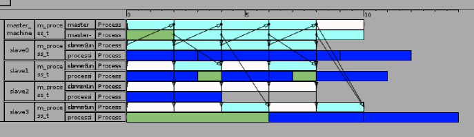
Figure 19: Trace of the simulation of BBA.

MBBSA achieves as expected the optimal makespan of 13 (see Figure 20). As you can see by comparing Figures 19 and 20, the second task scheduled by MBBSA (to worker $P_{2}$) is finished processing later than in the schedule of BBA. So MBBSA, while globally optimal, does not minimize the completion time of each task.

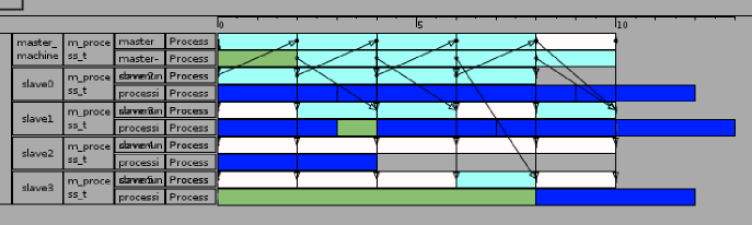
Figure 20: Trace of the simulation of MBBSA.

R-BSA finds also an optimal schedule (cf. Figure 21). Even in this small test the difference of R-BSA and MBBSA is remarkable: R-BSA tries to schedule the most tasks as possible by filling idle times starting at the makespan. MBBSA contrarily tries to schedule tasks as soon as possible before their deadlines are expired.

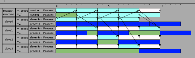
Figure 21: Trace of the simulation of R-BSA.

4.3 Distance from the best

We made a series of distance tests to get some information of the mean qualitiy of our algorithms. For this purpose we ran all algorithms on 1000 different random platforms of the each type, i.e., homogeneous and heterogeneous, as well as homogeneous communication links with heterogeneous workers and the converse. We normalized the measured schedule makespans over the best result for a given instance. In the following figures we plot the accumulated number of platforms that have a normalized distance less than the indicated distance. This means, we count on how many platforms a certain algorithm achieves results that do not differ more than X% from the best schedule. For exemple in Figure 22(b): The third point of the R-BSA-line significates that about 93% of the schedules of R-BSA differ less than 3% from the best schedule.

Our results on homogeneous platforms can be seen in Figures 22. As expected from the theoretical results, BBA and MBBSA achieve the same results and behave equally well on all platforms. R-BSA in contrast shows a sensibility on the platform characteristics. When the communication power is less than the computation power, i.e. the $c_{i}$-values are bigger, R-BSA behaves as good as MBBSA and BBA. But in the case of small $c_{i}$-values or on homogeneous platforms without constraints on the power rates, R-BSA achieves worse results.

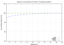
(a) Homogeneous platform (general case).

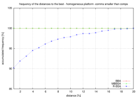
(b) Homogeneous platform, faster communicating.

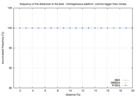
(c) Homogeneous platform, faster computing.

       

Figure 22: Frequency of the distance to the best on homogeneous platforms.

The simulation results on platforms with homogeneous communication links and heterogeneous computation powers (cf. Figure 23) consolidate the theoretical predictions: Independently of the platform parameters, MBBSA always obtains optimal results, BBA differs slightly when high precision is demanded. The behavior of R-BSA strongly depends on the platform parameters: when communications are slower than computations, it achieves good results.

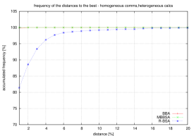
(a) General platform.

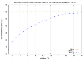
(b) Faster communicating.

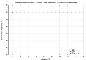
(c) Faster computing.

       

Figure 23: Frequency of the distance to the best on platforms with homogeneous communication links and heterogeneous computation power.

On platforms with heterogeneous communication links and homogeneous workers, BBA has by far the poorest results, whereas R-BSA shows a good behavior (see Figure 24). In general it outperforms MBBSA, but when the communication links are fast, MBBSA is the best.

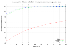
(a) General platform.

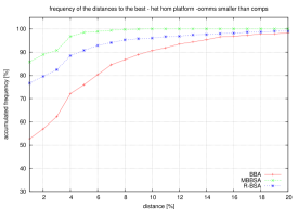
(b) Faster communicating.

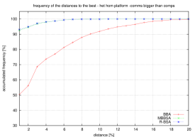
(c) Faster computing.

       

Figure 24: Frequency of the distance to the best on platforms with heterogeneous communication links and homogeneous computation power.

The results on heterogeneous platforms are equivalent to these on platforms with heterogeneous communication links and homogeneous workers, as can be seen in Figure 25. R-BSA seems to be a good candidate, whereas BBA is to avoid as the gap is up to more than 40%.

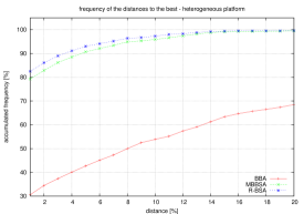
(a) Heterogeneous platform (general case).

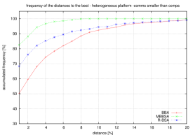
(b) Heterogeneous platform, faster communicating.

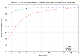
(c) Heterogeneous platform, faster computing.

       

Figure 25: Frequency of the distance to the best on heterogeneous platforms.

4.4 Mean distance and standard deviation

We also computed for every algorithm the mean distance from the best on each platform type. These calculations are based on the simulation results on the 1000 random platforms of Section 4.3. As you can see in Table 1 in general MBBSA achieves the best results. On homogeneous platforms BBA behaves just as well as MBBSA and on platforms with homogeneous communication links it also performs as well. When communication links are heterogeneous and there is no knowledge about platform parameters, R-BSA outperforms the other algorithms and BBA is by far the worse choice.

Platform type			Mean distance			Standard deviation
Comm.	Comp.		BBA	MBBSA	R-BSA	BBA	MBBSA	R-BSA
Hom	Hom		1	1	1.0014	0	0	0.0107
Hom	Hom	$c\leq w$	1	1	1.0061	0	0	0.0234
Hom	Hom	$c\geq w$	1	1	1	0	0	0
Hom	Het		1.0000	1	1.0068	0.0006	0	0.0181
Hom	Het	$c\leq w$	1.0003	1	1.0186	0.0010	0	0.0395
Hom	Het	$c\geq w$	1	1	1.0017	0	0	0.0040
Het	Hom		1.1894	1.0074	1.0058	0.4007	0.0208	0.0173
Het	Hom	$c\leq w$	1.0318	1.0049	1.0145	0.0483	0.0131	0.0369
Het	Hom	$c\geq w$	1.0291	1.0025	1.0024	0.0415	0.0097	0.0095
Het	Het		1.2100	1.0127	1.0099	0.3516	0.0327	0.0284
Het	Het	$c\leq w$	1.0296	1.0055	1.0189	0.0450	0.0127	0.0407
Het	Het	$c\geq w$	1.0261	1.0045	1.0046	0.0384	0.0118	0.0121

Table 1: Mean distance from the best and standard deviation of the different algorithms on each platform type.

The standard deviations of all algorithms over the 1000 platforms are shown in the right part of Table 1. These values mirror exactly the same conclusions as the listing of the mean distances in the left part, so we do not comment on them particularly. We only want to point out that the standard deviation of MBBSA always keeps small values, whereas in case of heterogeneous communication links BBA-heuristic is not recommendable.

5 Load balancing of divisible loads using the multiport switch-model

5.1 Framework

In this section we work with a heterogeneous star network. But in difference to Section 3 we replace the master by a switch. So we have $m$ workers which are interconnected by a switch and $m$ heterogenous links. Link $i$ is the link that connects worker $P_{i}$ to the switch. Its bandwidth is denoted by $b_{i}$. In the same way $s_{i}$ denotes the computation speed of worker $P_{i}$. Every worker $P_{i}$ possesses an amount of initial load $\alpha_{i}$. Contrarily to the previous section, this load is not considered to consist of identical and independent tasks but of divisible loads. This means that an amount of load $X$ can be divided into an arbitrary number of tasks of arbitrary size. As already mentioned, this approach is called Divisible Load Theory - DLT [4]. The communication model used in this case is an overlapped unbounded switched-multiport model. This means all communications pass by a centralized switch that has no throughput limitations. So all workers can communicate at the same time and a given worker can start executing as soon as it receives the first bit of data. As we use a model with overlap, communication and computation can take place at the same time.

As in the previous section our objective is to balance the load over the participating workers to minimize the global makespan $M$.

5.2 Redistribution strategy

Let $\sigma$ be a solution of our problem that takes a time $T$. In this solution, there is a set of sending workers $S$ and a set of receiving workers $R$. Let $send_{i}$ denote the amount of load sent by sender $P_{i}$ and $recv_{j}$ be the amount of load received by receiver $P_{j}$, with $send_{i}\geq 0$, $recv_{j}\geq 0$. As all load that is sent has to be received by another worker, we have the following equation:

$$\sum_{i\in S}send_{i}=\sum_{j\in R}recv_{j}=L.$$ (1)

In the following we describe the properties of the senders: As the solution $\sigma$ takes a time $T$, the amount of load a sender can send depends on its bandwidth: So it is bounded by the time-slot of

$$\forall\;\textnormal{sender}_{i}\in S,\hskip 28.45274pt\frac{send_{i}}{b_{i}}\leq T.$$ (2)

Besides, it has to send at least the amount of load that it can not finish processing in time $T$. This lowerbound can be expressed by

$$\forall\;\textnormal{sender}_{i}\in S,\hskip 28.45274ptsend_{i}\geq\alpha_{i}-T\times s_{i}.$$ (3)

The properties for receiving workers are similar. The amount of load a worker can receive is dependent of its bandwidth. So we have:

$$\forall\;\textnormal{receiver}_{j}\in R,\hskip 28.45274pt\frac{recv_{j}}{b_{j}}\leq T.$$ (4)

Additionally it is dependent of the amount of load it already possesses and of its computation speed. It must have the time to process all its load, the initial one plus the received one. That is why we have a second upperbound:

$$\forall\;\textnormal{receiver}_{j}\in S,\hskip 28.45274pt\frac{\alpha_{j}+recv_{j}}{s_{j}}\leq T.$$ (5)

For the rest of our paper we introduce a new notation: Let $\delta_{i}$ denote the imbalance of a worker. We will define it as follows:

$$\delta_{i}=\begin{cases}send_{i}&\text{if $i\in S$}\\ -recv_{i}&\text{if $i\in R$}\end{cases}$$

.

With the help of this new notation we can re-characterize the imbalance of all workers:

• This imbalance is bounded by

  $$|\delta_{i}|\leq b_{i}\times T.$$

  • If $i\in S$, worker $P_{i}$ is a sender, and this statement is true because of inequality 2.

  • If $i\in R$, worker $P_{i}$ is a receiver and the statement is true as well, because of inequality 4.

• Furthermore, we lower-bound the imbalance of a worker by

  $$\delta_{i}\geq\alpha_{i}-T\times s_{i}.$$ (6)

  • If $i\in S$, we are in the case where $\delta_{i}=send_{i}$ and hence this it true because of equation 3.

  • If $i\in R$, we have $\delta_{i}=-recv_{i}\leq 0$. Hence we get that (6) is equal to $-recv_{i}\geq\alpha_{i}-T\times s_{i}$ which in turn is equivalent to (5).

• Finally we know as well that $\sum_{i}\delta_{i}=0$ because of equation 1.

If we combine all these constraints we get the following linear program (LP), with the addition of our objective to minimize the makespan $T$. This combination of all properties into a LP is possible because we can use the same constraints for senders and receivers. As you may have noticed, a worker will have the functionality of a sender if its imbalance $\delta_{i}$ is positive, receivers being characterized by negative $\delta_{i}$-values.

$$\begin{array}[]{l}\textsc{Minimize }T,\\ \textsc{under the constraints}\\ \begin{cases}\ltx@label{min_{m}akespan}\begin{aligned} \tagform@{7a}\quad&|\delta_{i}|\leq T\times b_{i}\\ \tagform@{7b}\quad&\delta_{i}\geq\alpha_{i}-T\times s_{i}\\ \tagform@{7c}\quad&\sum_{i}\delta_{i}=0\end{aligned}\end{cases}\end{array}$$ (7)

All the constraints of the LP are satisfied for the $(\delta_{i},T)$-values of any schedule solution of the initial problem. We call $T_{0}$ the solution of the LP for a given problem. As the LP minimizes the time $T$, we have $T_{0}\leq T$ for all valid schedule and hence we have found a lower-bound for the optimal makespan.

Now we prove that we can find a feasible schedule with makespan $T_{0}$. We start from an optimal solution of the LP, i.e., $T_{0}$ and the $\delta_{i}$-values computed by some LP solvers, such as Maple or MuPAD. With the help of these found values we are able to describe the schedule:

1. Every sender $i$ sends a fraction of load to each receiver $j$. We decide that each sender sends to each receiver a fraction of the senders load proportional to what we denote by

   $$f_{i,j}=\delta_{i}\times\frac{\delta_{j}}{\sum_{k\in R}\delta_{k}}=\delta_{i}\times\frac{\delta_{j}}{-L}$$ (8)

   the fraction of load that a sender $P_{i}$ sends to a receiver $P_{j}$. In other words we have $f_{i,j}=\delta_{i}\times\frac{-recv_{i}}{\sum_{k\in R}(-recv_{k})}$.

2. During the whole schedule we use constant communication rates, i.e., worker $j$ will receive its fraction of load $f_{i,j}$ from sender $i$ with a fixed receiving rate, which is denoted by $\lambda_{i,j}$:

   $$\lambda_{i,j}=\frac{f_{i,j}}{T_{0}}.$$ (9)

3. A schedule starts at time $t=0$ and ends at time $t=T_{0}$.

We have to verify that each sender can send its amount of load in time $T_{0}$ and that the receivers can receive it as well and compute it afterwards.

Let us take a look at a sender $P_{i}$: the total amount it will send is $\sum_{j\in R}f_{i,j}=\sum_{j\in R}\frac{\delta_{i}\times\delta_{j}}{\sum_{k\in R}\delta_{k}}=\delta_{i}=send_{i}$ and as we started by a solution of our LP, $\delta_{i}$ respects equations LABEL:min_makespana and LABEL:min_makespanb, thus $send_{i}$ respects the constraints 2 and 3 as well, i.e., $send_{i}\leq T\times b_{i}$ and $send_{i}\geq\alpha_{i}-T\times s_{i}$.

Now we consider a receiver $P_{j}$: the total amount it will receive is $\sum_{i\in S}f_{i,j}=\sum_{i\in S}\frac{\delta_{i}\times\delta_{j}}{\sum_{k\in R}\delta_{k}}=-\delta_{j}=recv_{j}$. Worker $P_{i}$ can receive the whole amount of $recv_{i}$ load in time $T_{0}$ as it starts the reception at time $t=0$ and $recv_{i}$ respects constraints LABEL:min_makespana and LABEL:min_makespanb, who in turn respect the initial constraints 4 and 5, i.e., $recv_{i}\leq T\times b_{i}$ and $recv_{i}\leq T\times s_{i}-\alpha_{i}$. Now we examine if worker $P_{i}$ can finish computing all its work in time. As we use the divisible load model, worker $P_{i}$ can start computing its additional amount of load as soon as it has received its first bit and provided the computing rate is inferior to the receiving rate. Figure 26 illustrates the computing process of a receiver. There are two possible schedules: the worker can allocate a certain percentage of its computing power for each stream of loads and process them in parallel. This is shown in Figure 26(a). Processor $P_{i}$ starts immediately processing all incoming load. For doing so, every stream is allocated a certain computing rate $\gamma_{i,j}$, where $i$ is the sending worker and $j$ the receiver. We have to verify that the computing rate is inferior or equal to the receiving rate.

The initial load $\alpha_{j}$ of receiver $P_{j}$ owns at minimum a computing rate such that it finishes right in time $T_{0}$: $\gamma_{j,j}=\frac{\alpha_{j}}{T_{0}}$. The computing rate $\gamma_{i,j}$, for all pairs $(i,j)$, $i\in S$, $j\in R$, has to verify the following constraints:

• The sum of all computing rates does not exceed the computing power $s_{j}$ of the worker $P_{j}$:

  $$\left(\sum_{i\in S}\gamma_{i,j}\right)+\frac{\alpha_{j}}{T_{0}}\leq s_{j},$$ (10)

• The computing rate for the amount of load $f_{i,j}$ has to be sufficiently big to finish in time $T_{0}$:

  $$\gamma_{i,j}\geq\frac{f_{i,j}}{T_{0}},$$ (11)

• The computing rate has to be inferior or equal to the receiving rate of the amount $f_{i,j}$:

  $$\gamma_{i,j}\leq\lambda_{i,j},$$ (12)

Now we prove that $\gamma_{i,j}=\frac{f_{i,j}}{T_{0}}$ is a valid solution that respects constraints (10), (11), and (12):

Equation (10)

We have $\left(\sum_{i\in S}\gamma_{i,j}\right)+\frac{\alpha_{j}}{T_{0}}=\left(\sum_{i\in S}\frac{f_{i,j}}{T_{0}}\right)+\frac{\alpha_{j}}{T_{0}}=\left(\frac{-\delta_{j}}{T_{0}}\right)+\frac{\alpha_{j}}{T_{0}}=\frac{\alpha_{j}-\delta_{j}}{T_{0}}$. Transforming Equation (LABEL:min_makespanb) in $\alpha_{j}-\delta_{j}\leq T_{0}\times s_{j}$ and using this upperbound we get $\frac{\alpha_{j}-\delta_{j}}{T_{0}}\leq\frac{T_{0}\times s_{j}}{T_{0}}=s_{j}$. Hence this constraint holds true.

Equation (11)

By definition of $\gamma_{i,j}$ this holds true.

Equation (12)

By the definitions of $\gamma_{i,j}$ and $\lambda_{i,j}$ this holds true.

In the other possible schedule, all incoming load streams are processed in parallel after having processed the initial amount of load as shown in Figure 26(b). In fact, this modeling is equivalent to the precedent one, because we use the DLT paradigm. We used this model in equations 3 and 5.

(a) Parallel processing.

(b) Sequential and parallel processing.

   

Figure 26: Different schedules to process the received load.

The following theorem summarizes our cognitions:

Theorem 4.

The combination of the linear program LABEL:min_makespan with equations 8 and 9 returns an optimal solution for makespan minimization of a load balancing problem on a heterogeneous star platform using the switch model and initial loads on the workers.

6 Conclusion

In this report we were interested in the problem of scheduling and redistributing data on master-slave platforms. We considered two types of data models.

Supposing independent and identical tasks, we were able to prove the NP completeness in the strong sense for the general case of completely heterogeneous platforms. Therefore we restricted this case to the presentation of three heuristics. We have also proved that our problem is polynomial when computations are negligible. Treating some special topologies, we were able to present optimal algorithms for totally homogeneous star-networks and for platforms with homogeneous communication links and heterogeneous workers. Both algorithms required a rather complicated proof.

The simulative experiments consolidate our theoretical results of optimality. On homogeneous platforms, BBA is to privilege over MBBSA, as the complexity is remarkably lower. The tests on heterogeneous platforms show that BBA performs rather poorly in comparison to MBBSA and R-BSA. MBBSA in general achieves the best results, it might be outperformed by R-BSA when platform parameters have a certain constellation, i.e., when workers compute faster than they are communicating.

Dealing with divisible loads as data model, we were able to solve the fully heterogeneous problem. We presented the combination of a linear program with simple computation formulas to compute the imbalance in a first step and the corresponding schedule in a second step.

A natural extension of this work would be the following: for the model with independent tasks, it would be nice to derive approximation algorithms, i.e., heuristics whose worst-case is guaranteed within a certain factor to the optimal, for the fully heterogeneous case. However, it is often the case in scheduling problems for heterogeneous platforms that approximation ratios contain the quotient of the largest platform parameter by the smallest one, thereby leading to very pessimistic results in practical situations.

More generally, much work remains to be done along the same lines of load-balancing and redistributing while computation goes on. We can envision dynamic master-slave platforms whose characteristics vary over time, or even where new resources are enrolled temporarily in the execution. We can also deal with more complex interconnection networks, allowing slaves to circumvent the master and exchange data directly.

References

- [1] D. Altilar and Y. Paker. Optimal scheduling algorithms for communication constrained parallel processing. In Euro-Par 2002, LNCS 2400, pages 197–206. Springer Verlag, 2002.
- [2] O. Beaumont, L. Marchal, and Y. Robert. Scheduling divisible loads with return messages on heterogeneous master-worker platforms. Technical Report 2005-21, LIP, ENS Lyon, France, May 2005.
- [3] A. Bevilacqua. A dynamic load balancing method on a heterogeneous cluster of workstations. Informatica, 23(1):49–56, 1999.
- [4] V. Bharadwaj, D. Ghose, and T. Robertazzi. Divisible load theory: a new paradigm for load scheduling in distributed systems. Cluster Computing, 6(1):7–17, 2003.
- [5] Berkeley Open Infrastructure for Network Computing. http://boinc.berkeley.edu.
- [6] P. Brucker. Scheduling Algorithms. Springer-Verlag New York, Inc., Secaucus, NJ, USA, 2004.
- [7] M. Cierniak, M. Zaki, and W. Li. Customized dynamic load balancing for a network of workstations. Journal of Parallel and Distributed Computing, 43:156–162, 1997.
- [8] M. Drozdowski and L. Wielebski. Efficiency of divisible load processing. In PPAM, pages 175–180, 2003.
- [9] P. Dutot. Algorithmes d’ordonnancement pour les nouveaux supports d’exécution. PhD thesis, Laboratoire ID-IMAG, Institut National Polytechnique de Grenoble, 2004.
- [10] P. Dutot. Complexity of master-slave tasking on heterogeneous trees. European Journal of Operational Research, 164:690–695, 2005.
- [11] Einstein@Home. http://einstein.phys.usm.edu.
- [12] M. R. Garey and D. S. Johnson. Computers and Intractability, a Guide to the Theory of NP-Completeness. W.H. Freeman and Company, 1979.
- [13] D. Ghose. Feedback strategy for load allocation in workstation clusters with unknown network resource capabilities using the DLT paradigm. In Proceedings of the Parallel and Distributed Processing Techniques and Applications (PDPTA’02), volume 1, pages 425–428. CSREA Press, 2002.
- [14] M. Hamdi and C. Lee. Dynamic load balancing of data parallel applications on a distributed network. In 9th International Conference on Supercomputing ICS’95, pages 170–179. ACM Press, 1995.
- [15] U. Kremer. NP-Completeness of dynamic remapping. In Proceedings of the Fourth Workshop on Compilers for Parallel Computers, Delft, The Netherlands, 1993. Also available as Rice Technical Report CRPC-TR93330-S.
- [16] A. Legrand, L.Marchal, and H. Casanova. Scheduling Distributed Applications: The SimGrid Simulation Framework. In Proceedings of the Third IEEE International Symposium on Cluster Computing and the Grid (CCGrid’03), pages 138–145, May 2003.
- [17] M. A. Moges, T. G. Robertazzi, and D. Wu. Divisible load scheduling with multiple sources: Closed form solutions. In T. J. H. University, editor, Conference on Infomation Sciences and Systems, March 2005.
- [18] J. Moore. An n job, one machine sequencing algorithm for minimizing the number of late jobs. Management Science, 15(1), Sept. 1968.
- [19] M. Nibhanupudi and B. Szymanski. Bsp-based adaptive parallel processing. In R. Buyya, editor, High Performance Cluster Computing. Volume : Architecture and Systems, pages 702–721. Prentice-Hall, 1999.
- [20] H. Renard, Y. Robert, and F. Vivien. Data redistribution algorithms for heterogeneous processor rings. Research Report RR-2004-28, LIP, ENS Lyon, France, May 2004. Available at the url http://graal.ens-lyon.fr/~yrobert.
- [21] T. Robertazzi. Ten reasons to use divisible load theory. IEEE Computer, 36(5):63–68, 2003.
- [22] SETI. URL: http://setiathome.ssl.berkeley.edu.
- [23] B. A. Shirazi, A. R. Hurson, and K. M. Kavi. Scheduling and load balancing in parallel and distributed systems. IEEE Computer Science Press, 1995.
- [24] SimGrid. URL: http://simgrid.gforge.inria.fr.
- [25] M.-Y. Wu. On runtime parallel scheduling for processor load balancing. IEEE Trans. Parallel and Distributed Systems, 8(2):173–186, 1997.