Technical Report IDSIA-16-06  
Fitness Uniform Optimization
 

Abstract

In evolutionary algorithms, the fitness of a population increases with time by mutating and recombining individuals and by a biased selection of more fit individuals. The right selection pressure is critical in ensuring sufficient optimization progress on the one hand and in preserving genetic diversity to be able to escape from local optima on the other hand. Motivated by a universal similarity relation on the individuals, we propose a new selection scheme, which is uniform in the fitness values. It generates selection pressure toward sparsely populated fitness regions, not necessarily toward higher fitness, as is the case for all other selection schemes. We show analytically on a simple example that the new selection scheme can be much more effective than standard selection schemes. We also propose a new deletion scheme which achieves a similar result via deletion and show how such a scheme preserves genetic diversity more effectively than standard approaches. We compare the performance of the new schemes to tournament selection and random deletion on an artificial deceptive problem and a range of NP-hard problems: traveling salesman, set covering and satisfiability.

Keywords Evolutionary algorithms, fitness uniform selection scheme, fitness uniform deletion scheme, preserve diversity, local optima, evolution, universal similarity relation, correlated recombination, fitness tree model, traveling salesman, set covering, satisfiability

1 Introduction

1.1 Evolutionary algorithms (EA)

Evolutionary algorithms are capable of solving complicated optimization tasks in which an objective function $f:I\to{I\mskip-3.0mu\mskip-3.0muR}$ shall be maximized. $i\in I$ is an individual from the set $I$ of feasible solutions. Infeasible solutions due to constraints may also be considered by reducing $f$ for each violated constraint. A population $P$ is a multi-set of individuals from $I$ which is maintained and updated as follows: one or more individuals are selected according to some selection strategy. In generation based EAs, the selected individuals are recombined (e.g. crossover) and mutated, and constitute the new population. We prefer the more incremental, steady-state population update, which selects (and possibly deletes) only one or two individuals from the current population and adds the newly recombined and mutated individuals to it. We are interested in finding a single individual of maximal objective value $f$ for difficult multi-modal and deceptive problems.

1.2 Standard selection schemes (STD)

The standard selection schemes (abbreviated by STD in the following), proportionate, truncation, ranking and tournament selection all favor individuals of higher fitness [Gol89, GD91, BT95, BT97]. This is also true for less common schemes, like Boltzmann selection [MT93]. The fitness function is identified with the objective function (possibly after a monotone transformation). In linear proportionate selection the probability of selecting an individual depends linearly on its fitness [Hol75]. In truncation selection the $\alpha\%$ fittest individuals are selected, usually with multiplicity ${1\over\alpha\%}$ to keep the population size fixed [MSV94].(Linear) ranking selection orders the individuals according to their fitness. The selection probability is, then, a (linear) function of the rank [Whi89]. Tournament selection [Bak85], which selects the best $l$ out of $k$ individuals has primarily developed for steady-state EAs, but can be adapted to generation based EAs. All these selection schemes have the property (and goal!) to increase the average fitness of a population, i.e. to evolve the population toward higher fitness.

1.3 The problem of the right selection pressure

The standard selection schemes STD, together with mutation and recombination, evolve the population toward higher fitness. If the selection pressure is too high, the EA gets stuck in a local optimum, since the genetic diversity rapidly decreases. The suboptimal genetic material which might help in finding the global optimum is deleted too rapidly (premature convergence). On the other hand, the selection pressure cannot be chosen arbitrarily low if we want the EA to be effective. In difficult optimization problems, suitable population sizes, mutation and recombination rates, and selection parameters, which influence the selection intensity, are usually not known beforehand. Often, constant values are not sufficient at all [EHM99]. There are various suggestions to dynamically determine and adapt the parameters [Esh91, BHS91, Her92, SVM94]. Other approaches to preserve genetic diversity are fitness sharing [GR87] and crowding [Jon75]. They depend on the proper design of a neighborhood function based on the specific problem structure and/or coding. One approach which does not require a neighborhood function based on the genome is local mating [CJ91], however it has been shown that rapid takeover can still occur for basic spatial topologies [Rud00]. Another approach which has not been widely studied is preselection [Cav70].

We are interested in evolutionary algorithms which do not require special problem insight (problem specific neighborhood function and/or coding) and is able to effectively prevent population takeover. In this paper we introduce and analyze two potential approaches to this problem: the Fitness Uniform Selection Scheme (FUSS) and the Fitness Uniform Deletion Scheme (FUDS).

1.4 The fitness uniform selection scheme

FUSS is based on the insight that we are not primarily interested in a population converging to maximal fitness, but only in a single individual of maximal fitness. The scheme automatically creates a suitable selection pressure and preserves genetic diversity better than STD. The proposed fitness uniform selection scheme FUSS (see also Figure 1) is defined as follows: if the lowest/highest fitness values in the current population $P$ are $f_{min/max}$ we select a fitness value $f$ uniformly in the interval $[f_{min},f_{max}]$. Then, the individual $i\in P$ with fitness nearest to $f$ is selected and a copy is added to $P$, possibly after mutation and recombination. We will see that FUSS maintains genetic diversity better than STD, since a distribution over the fitness values is used, unlike STD, which all use a distribution over individuals. Premature convergence is avoided in FUSS by abandoning convergence at all. Nevertheless there is a selection pressure in FUSS toward higher fitness. The probability of selecting a specific individual is proportional to the distance to its nearest fitness neighbor. In a population with a high density of unfit and low density of fit individuals, the fitter ones are effectively favored.

1.5 The fitness uniform deletion scheme

We may also preserve diversity through deletion rather than through selection. By always deleting from those individuals which have very commonly occurring fitness values we achieve a population which is uniformly distributed across fitness values, like with FUSS. Because these deleted individuals are “commonly occurring” in some sense this should help preserve population diversity. Under FUDS the role of the selection scheme is to govern how actively different parts of the solution space are searched rather than to move the population as a whole toward higher fitness. Thus, like with FUSS, premature convergence is avoided by abandoning convergence as our goal. However as FUDS is only a deletion scheme, the EA still requires a selection scheme which may require a selection intensity parameter to be set. Thus we do not necessarily have a parameterless EA, as we do with FUSS. Nevertheless due to the impossibility of population collapse the performance is more robust than usual with respect to variation in selection intensity. Thus FUDS is at least a partial solution to the problem of having to correctly set a selection intensity parameter.

1.6 Contents

This paper extends and supersedes the earlier results reported in the conference papers [Hut02], [LHK04] and [LH05]. Among other things, this paper: extends the previous theoretical analysis of FUSS and gives the first theoretical analysis of FUDS and of their performance when combined; presents a new method of analysis called fitness tree analysis; is the first set of experimental results which directly compares the two proposed schemes on the same problems with the same parameters, including when they are used together; gives the first full analysis of population diversity measurements for FUSS and in particular extends and corrects some of the earlier speculation about performance problems in some situations.

The paper is structured as follows:

In Section 2 we discuss the problems of local optima and population takeover [GD91] in STD, which could be lowered by restricting the number of similar individuals in a population. As we often do not have an appropriate functional similarity relation, we define a universal distance (semi-metric) $d(i,j):=|f(i)-f(j)|$ based on the available fitness only, which will serve our needs.

Motivated by the universal similarity relation $d$ and by the need to preserve genetic diversity, we define in Section 3 the fitness uniform selection scheme. We discuss under which circumstances FUSS leads to an (approximate) fitness uniform population.

Further properties of FUSS are discussed in Section 4, especially, how FUSS creates selection pressure toward higher fitness and how it preserves diversity better than STD. Further topics are the equilibrium distribution, the transformation properties of FUSS under linear and non-linear transformations of $f$.

Another way to utilize the ability of the universal similarity relation $d$ to preserve diversity, is to use it to help target deletion. This gives us the fitness uniform deletion scheme which we define in Section 5. As this produces a population which is approximately uniformly distributed across fitness levels, like with FUSS, many of the properties of FUSS carry over to an EA using FUDS. Some of these properties are highlighted in Section 6.

In Section 7 we theoretically demonstrate, by way of a simple optimization example, that an EA with FUSS or FUDS can optimize much faster than with STD. We show that crossover can be effective in FUSS, even when ineffective in STD. Furthermore, FUSS, FUDS and STD are compared to random search with and without crossover.

In Section 8 we develop a fitness tree model, which we believe to cover the essential features of fitness landscapes for difficult problems with many local optima. Within this model we derive heuristic expressions for the optimization time of random walk, FUSS, FUDS and STD. They are compared, and a worst case slowdown of FUSS relative to STD is obtained.

There is a possible additional slowdown when including recombination, as discussed in Section 9, which can be avoided by using a scale independent pair selection. It is a “best” compromise between unrestricted recombination and recombination of $d$-similar individuals only. It also has other interesting properties when used without crossover.

To simplify the discussion we have concentrated on the case of discrete, equi-spaced fitness values. In many practical problems, the fitness function is continuously valued. FUSS and some of the discussion of the previous sections is generalized to the continuous case in Section 10.

Section 11 begins our experimental analysis of FUSS and FUDS. In this section we give a detailed account of the EA software we have used for our experiments, including links to where the source code can be downloaded.

Section 12 examines the empirical performance of FUSS and FUDS on the artificially constructed deceptive optimization problem described in Section 7. These results confirm the correctness of our theoretical analysis.

In Section 13 we test randomly generated traveling salesman problems.

In Section 14 we examine the set covering problem, an NP hard optimization problem which has many real world applications.

For our final test in Section 15 we look at random CNF3 SAT problems. These are also NP hard optimization problems.

Section 16 contains a summary of our results and possible avenues for future research.

2 Universal Similarity Relation

2.1 The problem of local optima

Proportionate, truncation, ranking and tournament are the standard (STD) selection algorithms used in evolutionary optimization. They have the following property: if a local optimum $i^{lopt}$ has been found, the number of individuals with fitness $f^{lopt}=f(i^{lopt})$ tends to increase rapidly. Assume a low mutation and recombination rate, or, for instance, truncation selection after mutation and recombination. Further, assume that it is very difficult to find an individual fitter than $i^{lopt}$. The population will then degenerate and will consist mostly of $i^{lopt}$ after a few rounds. This decreased diversity makes it even less likely that $f^{lopt}$ gets improved. The suboptimal genetic material which might help in finding the global optimum has been deleted too rapidly. On the other hand, too high mutation and recombination rates convert the EA into an inefficient random search.

2.2 Possible solution

Sometimes it is possible to appropriately choose the mutation and recombination rate and population size by some insight into the nature of the problem. More often this is a trial and error process, or no single fixed rate works at all.

A naive fix of the problem is to artificially limit the number of identical individuals to a significant but small fraction $\varepsilon$. If the space of individuals $I$ is large, there could be many very similar (but not identical) individuals of, for instance, fitness $f^{lopt}$. The EA can still converge to a population containing only this class of similar individuals, with all others becoming extinct. In order for the limitation approach to work, one has to restrict the number of similar individuals. Significant contributions in this direction are fitness sharing [GR87] and crowding [Jon75].

2.3 The problem of finding a similarity relation

If the individuals are coded binary one might use the Hamming distance as a similarity relation. This distance is consistent with a mutation operator which flips a few bits. It produces Hamming-similar individuals, but recombination (like crossover) can produce very dissimilar individuals w.r.t. this measure. In any case, genotypic similarity relations, like the Hamming distance, depend on the representation of the individuals as binary strings. Individuals with very dissimilar genomes might actually be functionally (phenotypically) very similar. For instance, when most bits are unused (like introns in genetic programming), they can be randomly disturbed without affecting the properties of the individual. For specific problems at hand, it might be possible to find suitable representation-independent functional similarity relations. On the other hand, in genetic programming, for instance, it is in general undecidable whether two individuals are functionally similar.

2.4 A universal similarity relation

Here we want to take a different approach. We define the difference or distance between two individuals as

$$d(i,j)\mskip 5.0mu plus 5.0mu:=\mskip 5.0mu plus 5.0mu|f(i)-f(j)|.$$

The distance is based solely on the fitness function, which is provided as part of the problem specification. It is independent of the coding/representation and other problem details, and of the optimization algorithm (e.g. the genetic mutation and recombination operators), and can trivially be computed from the fitness values. If we make the natural assumption that functionally similar individuals have similar fitness, they are also similar w.r.t. the distance $d$. On the other hand, individuals with very different coding, and even functionally dissimilar individuals may be $d$-similar, but we will see that this is acceptable. For instance, individuals from different local optima of equal height are $d$-similar.

2.5 Relation to niching and crowding

Unlike fitness uniform optimization, diversity control methods like niching or crowding require a metric $g$ to be defined over the genome space. By looking at the relationship between $g$ and $f$ we can relate these two types of diversity control: We say that a fitness function $f$ is smooth with respect to $g$, if $g(i,j)$ being small implies that $|f(i)-f(j)|$ is also small, that is, $d(i,j)$ is small. This implies that if $d(i,j)$ is not small, $g(i,j)$ also cannot be small. Thus, if we limit the number of $d$ similar individuals, as we do in fitness uniform optimization, this will also limit the number of $g$ similar individuals, as is done in crowding and niching methods. The advantage of fitness uniform optimization is that we do not need to know what $g$ is, or to compute its value. Indeed, the above argument is true for any metric $g$ on the genome space that $f$ is smooth with respect to.

On the other hand, if the fitness function $f$ is not generally smooth with respect to $g$, then such a comparison between the methods cannot be made. However, in this case an EA is less likely to be effective as small mutations in genome space with respect to $g$ will produce unpredictable changes in fitness.

2.6 Topologies on individual space $I$

The distance $d:I\times I\to{I\mskip-3.0mu\mskip-3.0muR}_{0}^{+}$ induced by the fitness function $f$ is a semi-metric on the individual space $I$ (semi only because $d(i,j)=0$ for $i\neq j$ is possible). The semi-metric induces a topology on $I$. Equal fitness suffices to declare two individuals as $d$-equivalent, i.e. $d$ is a rather small semi-metric in the sense that the induced topology is rather coarse. We will see that a non-zero distance between individuals of different fitness is sufficient to avoiding the population takeover. $d$ induces the coarsest topology (is the “smallest” distance) avoiding population takeover.

2.7 The problem of genetic drift

Besides elitist selection, the other major cause of diversity loss in a population is genetic drift. This occurs due to the stochastic nature of the selection operator breeding some individuals more often than others. In a finite population this will cause some individuals to be replaced which have no close relatives, thus reducing diversity. Indeed, without a sufficient rate of mutation, eventually a population will converge on a single genome; even if no selection pressure is applied.

Although fitness uniform optimization does not attempt to address this problem, some implications can be drawn. Clearly, with fitness uniform optimization a complete collapse in diversity is impossible as individuals with a wide range of fitness values are always preserved in the population. However, within a given fitness level genetic drift can occur, although the sustained presence of many individuals in other fitness levels to breed with will reduce this effect.

Theoretical analysis of genetic drift is often performed by calculating the Markov chain transition matrices to compute the time for the system to reach an absorption state where all of the population members have the same genome. As these results can be difficult to generalize, an alternative approach has been to measure genetic drift by measuring the loss in fitness diversity in a population over time [RPB99a]. This is interesting as fitness uniform optimization attempts to maximize the entropy of the fitness values in the population, producing a very high variance in population fitness. Thus, at least according to the second method of analysis, very little genetic drift would be evident in the population.

3 Fitness Uniform Selection Scheme (FUSS)

3.1 Discrete fitness function

In this section we propose a new selection scheme, which limits the fraction of $d$-similar individuals. For simplicity we start with a fitness function $f:I\to F$ with discrete equi-spaced values $F=\{f_{min},f_{min}+\varepsilon,f_{min}+2\varepsilon,...,f_{max}-\varepsilon,f_{max}\}$. We call two individuals $i$ and $j$ $\delta$-similar if $d(i,j)\equiv|f(i)-f(j)|\leq\delta$. The continuous valued case $F=[f_{min},f_{max}]$ is considered later. In the following we assume $\delta<\varepsilon$. In this case, two individuals are $\delta$-similar if and only if they have the same fitness.

3.2 The goal

We have argued that in order to escape local optima, genetic variety should be preserved somehow. One way is to limit the number of $\delta$-similar individuals in the population. In an exact fitness uniform distribution there would be $|P|/|F|$ individuals for each of the $|F|$ fitness values, i.e. each fitness level would be occupied by a fraction of $1/|F|$ individuals. The following selection scheme asymptotically transforms any finite population into a fitness uniform one.

3.3 The fitness uniform selection scheme (FUSS)

FUSS is defined as follows: randomly select a fitness value $f$ uniformly from the fitness values $F$. Then, uniformly at random select an individual $i\in P$ with fitness $f$. Add another copy of $i$ to $P$.

Note the two stage uniform selection process which is very different from a one step uniform selection of an individual of $P$ (see Figure 1).

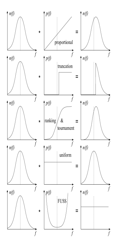
Figure 1: Effects of proportionate, truncation, ranking & tournament, uniform, and fitness uniform (FUSS) selection on the fitness distribution in a generation based EA. The left/right diagrams depict fitness distributions before/after applying the selection schemes depicted in the middle diagrams. Note that for populations with a non-Gaussian distribution of fitness values (left column), the graph of selection probability vs. fitness for FUSS (center bottom) can be totally different to that illustrated above, however the population distribution that results (right bottom) will be the same.

In STD, inertia increases with population size. A large mass of unfit individuals reduces the probability of selecting fit individuals. This is not the case for FUSS. Hence, without loss of performance, we can define a pure model, in which no individual is ever deleted; the population size increases with time. No genetic material is ever discarded and no fine-tuning in population size is necessary. What may prevent the pure model from being applied to practical problems are not computation time issues, but memory problems. If space becomes a problem we delete random individuals, as is usually done with a steady state EA.

3.4 Asymptotically fitness uniform distribution

The expected number of individuals per fitness level $f$ after $t$ selections is $n_{t}(f)=n_{0}(f)+t/|F|$, where $n_{0}(f)$ is the initial distribution. Hence, asymptotically each fitness level gets occupied uniformly by a fraction

$${n_{t}(f)\over|P_{t}|}\mskip 5.0mu plus 5.0mu=\mskip 5.0mu plus 5.0mu{n_{0}(f)+t/|F|\over|P_{0}|+t}\mskip 5.0mu plus 5.0mu\to\mskip 5.0mu plus 5.0mu{1\over|F|}\quad\mbox{for}\quad t\to\infty,$$

where $P_{t}$ is the population at time $t$. The same limit holds if each selection is accompanied by uniformly deleting one individual from the (now constant sized) population.

3.5 Fitness gaps and continuous fitness

We made two unrealistic assumptions. First, we assumed that each fitness level is initially occupied. If the smallest/largest fitness values in $P_{t}$ are $f_{min/max}^{t}$ we extend the definition of FUSS by selecting a fitness value $f$ uniformly in the interval $[f_{min}^{t}-{\textstyle{1\over 2}}\varepsilon,f_{max}^{t}+{\textstyle{1\over 2}}\varepsilon]$ and an individual $i\in P_{t}$ with fitness nearest to $f$ (see Figure 2). This also covers the case when there are missing intermediate fitness values, and also works for continuous valued fitness functions ($\varepsilon\to 0$).

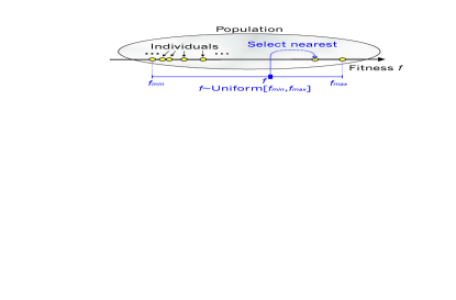
Figure 2: If the lowest/highest fitness values in the current population $P$ are $f_{min/max}$, FUSS selects a fitness value $f$ uniformly in the interval $[f_{min},f_{max}]$, then, the individual $i\in P$ with fitness nearest to $f$ is selected and a copy is added to $P$, possibly after mutation and recombination.

3.6 Mutation and recombination

The second assumption was that there is no mutation and recombination. In the presence of a small mutation and/or recombination rate eventually each fitness level will become occupied and the occupation fraction is still asymptotically approximately uniform. For larger rate the distribution will be no longer uniform, but the important point is that the occupation fraction of no fitness level decreases to zero for $t\to\infty$, unlike for STD. Furthermore, FUSS selects by construction uniformly in the fitness levels, even if the levels are not uniformly occupied.

4 Properties of FUSS

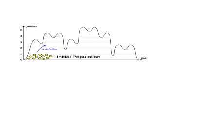
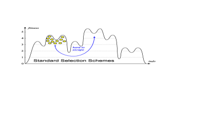
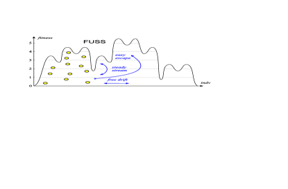
Figure 3: Evolution of the population under FUSS versus standard selection schemes (STD): STD may get stuck in a local optimum if all unfit individuals were eliminated too quickly. In FUSS, all fitness levels remain occupied with “free” drift within and in-between fitness levels, from which new mutants are steadily created, occasionally leading to further evolution in a more promising direction.

4.1 FUSS effectively favors fit individuals

FUSS preserves diversity better than STD, but the latter have a (higher) selection pressure toward higher fitness, which is necessary for optimization. At first glance it seems that there is no such pressure at all in FUSS, but this is deceiving. As FUSS selects uniformly in the fitness levels, individuals of low populated fitness levels are effectively favored. The probability of selecting a specific individual with fitness $f$ is inversely proportional to $n_{t}(f)$ (see Figure 1). In an initial typical (FUSS) population there are many unfit and only a few fit individuals. Hence, fit individuals are effectively favored until the population becomes fitness uniform. Occasionally, a new higher fitness level is discovered and occupied by a single new individual, which then, again, is favored.

4.2 No takeover in FUSS

With FUSS, takeover of the highest fitness level never happens. The concept of takeover time [GD91] is meaningless for FUSS. The fraction of fittest individuals in a population is always small. This implies that the average population fitness is always much lower than the best fitness. Actually, a large number of fit individuals is usually not the true optimization goal. A single fittest individual usually suffices to solve the optimization task.

4.3 FUSS may also favor unfit individuals

Note, if it is also difficult to find individuals of low fitness, i.e. if there are only a few individuals of low fitness, FUSS will also favor these individuals. Half of the time is “wasted” in searching on the wrong end of the fitness scale. This possible slowdown by a factor of 2 is usually acceptable. In Section 7 we will see that in certain circumstances this behavior can actually speedup the search. In general, fitness levels which are difficult to reach, are favored.

4.4 Distribution within a fitness level

Within a fitness level there is no selection pressure which could further exponentially decrease the population in certain regions of the individual space. This (exponential) reduction is the major enemy of diversity, which is suppressed by FUSS. Within a fitness level, the individuals freely drift around (by mutation). Furthermore, there is a steady stream of individuals into and out of a level by (d)evolution from (higher)lower levels. Consequently, FUSS develops an equilibrium distribution which is nowhere zero. This does not mean that the distribution within a level is uniform. For instance, if there are two (local) maxima of same height, a very broad one and a very narrow one, the broad one may be populated much more than the narrow one, since it is much easier to “find”.

4.5 Steady creation of individuals from every fitness level

In STD, a wrong step (mutation) at some point in evolution might cause further evolution in the wrong direction. Once a local optimum has been found and all unfit individuals were eliminated it is very difficult to undo the wrong step. In FUSS, all fitness levels remain occupied from which new mutants are steadily created, occasionally leading to further evolution in a more promising direction (see Figure 3).

4.6 Transformation properties of FUSS

FUSS (with continuous fitness) is independent of a scaling and a shift of the fitness function, i.e. FUSS($\tilde{f}$) with $\tilde{f}(i):=a\cdot f(i)+b$ is identical to FUSS($f$). This is true even for $a<0$, since FUSS searches for maxima and minima, as we have seen. It is not independent of a non-linear (monotone) transformation unlike tournament, ranking and truncation selection. The non-linear transformation properties are more like the ones of proportionate selection.

5 Fitness Uniform Deletion Scheme (FUDS)

For a steady state evolutionary algorithm each cycle of the system consists of both selecting which individual or individuals to crossover and mutate, and then selecting which individual is to be deleted in order to make space for the new child. The usual deletion scheme used is random deletion as this is neutral in the sense that it does not bias the distribution of the population in any way and does not require additional work to be done, such as evaluating the similarity of individuals based on their genes. Another common strategy is to use an elitist deletion scheme.

Here we propose to use the similarity semi-metric $d$ defined in Section 2 to achieve a uniform distribution across fitness levels, like with FUSS, except that we achieve this by selectively deleting those members of the population which have very commonly occurring fitness values. Of course this leaves the selection scheme unspecified, indeed we may use any standard selection scheme such as tournament selection in combination with FUDS. It also means that we lose one of the nice features of FUSS as we now need to manually tune the selection intensity for our application — FUSS of course is parameterless. Nevertheless it allows us to give many FUSS like properties to an existing EA using a standard selection scheme with only a minor modification to the deletion scheme.

The intuition behind why FUDS preserves population diversity is very simple: If an individual has a fitness value which is very rare in the population then this individual almost certainly contains unique information which, if it were to be deleted, would decrease the total population diversity. Conversely, if we delete an individual with very commonly occurring fitness then we are unlikely to be losing significant diversity. Presumably most of these individuals are common in some sense and likely exist in parts of the solution space which are easy to reach. Thus the fitness uniform deletion strategy is now clear: Only delete individuals with very commonly occurring fitness values as these individuals are less likely to contain important genetic diversity.

Practically FUDS is implemented as follows. Let $f_{min}$ and $f_{max}$ be the minimum and maximum fitness values possible for a problem, or at least reasonable upper and lower bounds. We divide the interval $[f_{min},f_{max}]$ into a collection of subintervals of equal length $\{[f_{min},f_{min}+a),[f_{min}+a,f_{min}+2a),\ldots,[f_{max}-a,f_{max}]\}$ which we call fitness levels. As individuals are added to the population their fitness is computed and they are placed in the set of individuals corresponding to the fitness level they belong to. Thus the number of individuals in each fitness level describes how common fitness values within this interval are in the current population. When a deletion is required the algorithm locates the fitness level with the greatest number of individuals and then deletes a random individual from this level. In the case where multiple fitness levels have maximal size the lowest of these levels is used.

If the number of fitness levels is chosen too low, say 5 levels, then the resulting model of the distribution of individuals across the fitness range will be too coarse. Alternatively if a large number of fitness levels is used with a very small population the individuals may become too thinly spread across the fitness levels. While in these extreme cases this could affect the performance of FUDS, in practice we have found that the system is not very sensitive to the setting of this parameter. If $n$ is the population size then setting the number of fitness levels to be $\sqrt{n}$ is a good rule of thumb.

For discrete valued fitness functions there is a natural lower bound on the interval length $a$ because below a certain value there will be more intervals than unique fitness values. Of course this cannot happen when the fitness function is continuous. Other than this small technical detail, the two cases are treated identically.

As FUDS spreads the individuals out across a wide range of fitness values, for small populations the EA may become inefficient as only a few individuals will have relatively high fitness. For problems which are not deceptive this is especially true as there will be little value in having individuals in the population with low to medium fitness. Of course these are not the kinds of problems for which FUDS was designed. In practice we have always used populations of between 250 and 5,000 individuals and have not observed a decline in performance relative to random deletion at the lower end of this range.

An alternative implementation that avoids discretization is to choose the two individuals that have the most similar fitness and delete one of them. An efficient implementation keeps a list of the individuals ordered by their fitness along with an ordered list of the distances between the individuals. Then in each cycle one of the two individuals with closest fitness to each other is selected for deletion. Although the performance of this algorithm was better than random deletion, it was not as good as the implementation of FUDS using bins. We conjecture that the reason for this is as follows: When there are just a few very fit individuals in the population it is quite likely that they will be highly related to each other and have very similar fitness. This means that if we delete the individuals with most similar fitness it is likely that many of the very fit individuals will be deleted. However with the bins approach this will not happen as there are typically few individuals in the high fitness bins. Thus, although deleting one of the closest individuals in terms of fitness might preserve diversity well, it also changes the pressure on the population distribution over fitness levels. This small change in distribution dynamics appears to reduce performance in practice.

6 Properties of FUDS

As FUDS uniformly distributes the population across fitness levels, like FUSS does, many of the key properties of FUSS also carry over to an EA that is using a standard selection scheme (STD) combined with FUDS deletion.

6.1 No takeover in FUDS

Under FUDS the takeover of the highest fitness level, or indeed any fitness level, is impossible. This is easy to see because as soon as any fitness level starts to dominate, all of the deletions become focused on this level until it is no longer the most populated fitness level. As a by-product, this also means that individuals on relatively unpopulated fitness levels are preserved.

6.2 Steady creation of individuals from every fitness level

Another similarity with FUSS is the steady creation of individuals on many different fitness levels. This occurs because under FUDS some individuals on each fitness level are always kept. This makes it relatively easy for the EA to find its way out of local optima as it keeps on exploring evolutionary paths which do not at first appear to be promising.

6.3 Robust performance with respect to selection intensity

Because FUDS is only a deletion scheme, we still need to choose a selection scheme for the EA. Of course this selection scheme may then require us to set a selection intensity parameter. While this is not as desirable as FUSS, which has no such parameter, at least with FUDS we expect the performance of the system to be less sensitive to the correct setting of this parameter. For example, if the selection intensity is set too high the normal problem is that the population rushes into a local optimum too soon and becomes stuck before it has had a chance to properly explore the genotype space for other promising regions. However, as we noted above, with FUDS a total collapse in population diversity is impossible. Thus much higher levels of selection intensity may be used without the risk of premature convergence.

In some situations if very low section intensity is used along with random deletion, the population tends not to explore the higher areas of the fitness landscape at all. This can be illustrated by a simple example. Consider a population which contains 1,000 individuals. Under random deletion all of these individuals, including the highly fit ones, will have a 1 in 1,000 chance of being deleted in each cycle and so the expected life time of an individual is 1,000 deletion cycles. Thus if a highly fit individual is to contribute a child of the same fitness or higher, it must do so reasonably quickly. However for some optimization problems the probability of a fit individual having such a child when it is selected is very low, so low in fact that it is more likely to be deleted before this happens. As a result the population becomes stuck, unable to find individuals of greater fitness before the fittest individuals are killed off.

The usual solution to this problem is to increase the selection intensity because then the fit individuals are selected more often and thus are more likely to contribute a child of similar or greater fitness before they are deleted. Another is to change the deletion scheme so that these individuals live longer. This is what happens with FUDS as rare fit individuals are not deleted. Effectively it means that with FUDS we can often use much lower selection intensity without the population becoming stuck.

6.4 Transformation properties of FUDS

While with FUDS we have the added complication of having to choose the number of subintervals with which to break up the fitness values, this number is only a function of the population size and distributional characteristics of the problem. Thus any linear transformation of the fitness function has no effect on FUDS. However, non-linear transformations will affect performance.

6.5 Problem and representation independence

Because FUDS only requires the fitness of individuals, the method is completely independent of the problem and genotype representation, i.e. how the individuals are coded.

6.6 Simple implementation and low computational cost

As the algorithm is simple and the fitness function is given as part of the problem specification, FUDS is very easy to implement and requires few computational resources.

7 A Simple Example

In the following, we use a simple example problem to compare the performance of fitness uniform selection (FUSS), random search (RAND) and standard selection (STD), each used both with and without recombination. We also examine the performance of standard selection when used with the fitness uniform deletion scheme (FUDS). We regard this problem as a prototype for deceptive multi-modal functions. The example demonstrates how FUSS and FUDS can be superior to RAND and STD in some situations. More generic situations will be considered in Section 8. An experimental analysis of this problem appears in Section 12.

7.1 Simple 2D example

Consider individuals $(x,y)\in I:=[0,1]\times[0,1]$, which are tuples of real numbers, each coordinate in the interval $[0,1]$. The example models individuals possessing up to 2 “features”. Individual $i$ possesses feature $I_{1}$ if $i\in I_{1}:=[a,a+\Delta]\times[0,1]$, and feature $I_{2}$ if $i\in I_{2}:=[0,1]\times[b,b+\Delta]$. The fitness function $f:I\to\{1,2,3\}$ is defined as

$$f(x,y)=\left\{\begin{array}[]{l}1\quad\mbox{if}\quad(x,y)\in I_{1}\backslash I_{2},\\ 2\quad\mbox{if}\quad(x,y)\in I_{2}\backslash I_{1},\\ 3\quad\mbox{if}\quad(x,y)\not\in I_{1}\cup I_{2},\\ 4\quad\mbox{if}\quad(x,y)\in I_{1}\cap I_{2}.\\ \end{array}\right.\parbox{56.9055pt}{\hfill\begin{picture}(45.0,45.0)\scriptsize\put(5.0,5.0){\vector(0,1){40.0}} \put(5.0,5.0){\vector(1,0){40.0}} \put(20.0,5.0){\line(0,1){35.0}} \put(25.0,5.0){\line(0,1){35.0}} \put(40.0,5.0){\line(0,1){35.0}} \put(5.0,15.0){\line(1,0){35.0}} \put(5.0,20.0){\line(1,0){35.0}} \put(5.0,40.0){\line(1,0){35.0}} \put(22.5,17.5){\makebox(0.0,0.0)[cc]{4}} \put(12.5,30.0){\makebox(0.0,0.0)[cc]{3}} \put(22.5,30.0){\makebox(0.0,0.0)[cc]{1}} \put(32.5,30.0){\makebox(0.0,0.0)[cc]{3}} \put(32.5,10.0){\makebox(0.0,0.0)[cc]{3}} \put(12.5,10.0){\makebox(0.0,0.0)[cc]{3}} \put(12.5,17.5){\makebox(0.0,0.0)[cc]{2}} \put(32.5,17.5){\makebox(0.0,0.0)[cc]{2}} \put(22.5,10.0){\makebox(0.0,0.0)[cc]{1}} \put(44.0,2.5){\makebox(0.0,0.0)[cc]{$x$}} \put(22.5,2.5){\makebox(0.0,0.0)[cc]{$\Delta$}} \put(20.0,3.5){\makebox(0.0,0.0)[cc]{$a$}} \put(2.5,17.5){\makebox(0.0,0.0)[cc]{$\Delta$}} \put(4.0,14.5){\makebox(0.0,0.0)[cc]{$b$}} \put(40.0,3.0){\makebox(0.0,0.0)[cc]{1}} \put(3.5,40.0){\makebox(0.0,0.0)[cc]{1}} \put(2.5,44.0){\makebox(0.0,0.0)[cc]{$y$}} \put(22.5,42.5){\makebox(0.0,0.0)[cc]{$f(x,y)$}} \end{picture} }$$

We assume $\Delta\ll 1$. Individuals with neither of the two features ($i\in I\backslash(I_{1}\cup I_{2})$) have fitness $f=3$. These “local $f=3$ optima” occupy most of the individual space $I$, namely a fraction $(1-\Delta)^{2}$. It is disadvantageous for an individual to possess only one of the two features ($i\in(I_{1}\backslash I_{2})\cup(I_{2}\backslash I_{1})$), since $f=1$ or 2 in this case. In combination ($i\in I_{1}\cap I_{2})$), the two features lead to the highest fitness, but the global maximum $f=4$ occupies the smallest fraction $\Delta^{2}$ of the individual space $I$. With a fraction $\Delta(1-\Delta)$, the $f=1/f=2$ minima are in between. The example has sort of an XOR structure, which is hard for many optimizers.

7.2 Random search

Individuals are created uniformly in the unit square. The “local optimum” $f=3$ is easy to “find”, since it occupies nearly the whole space. The global optimum $f=4$ is difficult to find, since it occupies only $\Delta^{2}\ll 1$ of the space. The expected time, i.e. the expected number of individuals created and tested until one with $f=4$ is found, is $T_{RAND}={1\over\Delta^{2}}$. Here and in the following, the “time” $T$ is defined as the expected number of created individuals until the first optimal individual (with $f=4$) is found. $T$ is neither a takeover time nor the number of generations (we consider steady-state EAs).

7.3 Random search with crossover

Let us occasionally perform a recombination of individuals in the current population. We combine the $x$-coordinate of one uniformly selected individual $i_{1}$ with the $y$ coordinate of another individual $i_{2}$. This crossover operation maintains a uniform distribution of individuals in $[0,1]^{2}$. It leads to the global optimum if $i_{1}\in I_{1}$ and $i_{2}\in I_{2}$. The probability of selecting an individual in $I_{i}$ is $\Delta(1-\Delta)\approx\Delta$ (we assumed that the global optimum has not yet been found). Hence, the probability that $I_{1}$ crosses with $I_{2}$ is $\Delta^{2}$. The time to find the global optimum by random search including crossover is still $\sim{1\over\Delta^{2}}$ ($\sim$ denotes asymptotic proportionality).

7.4 Mutation

The result remains valid (to leading order in ${1\over\Delta}$) if, instead of a random search, we uniformly select an individual and mutate it according to some probabilistic, sufficiently mixing rule, which preserves uniformity in $[0,1]$. One popular such mutation operator is to use a sufficiently long binary representation of each coordinate, like in genetic algorithms, and flip a single bit. For simplicity we assume in the following a mutation operator which replaces with probability ${\textstyle{1\over 2}}/{\textstyle{1\over 2}}$ the first/second coordinate by a new uniform random number. Other mutation operators which mutate with probability ${\textstyle{1\over 2}}/{\textstyle{1\over 2}}$ the first/second coordinate, preserve uniformity, are sufficiently mixing, and leave the other coordinate unchanged (like the single-bit-flip operator) lead to the same scaling of $T$ with $\Delta$ (but with different proportionality constants).

7.5 Standard selection with crossover

The $f=1$ and $f=2$ individuals contain useful building blocks, which could speedup the search by a suitable selection and crossover scheme. Unfortunately, the standard selection schemes favor individuals of higher fitness and will diminish the $f=1/f=2$ population fraction. The probability of selecting $f=1/f=2$ individuals is even smaller than in random search. Hence $T_{STD}\sim{1\over\Delta^{2}}$. Standard selection does not improve performance, even not in combination with crossover, although crossover is well suited to produce the needed recombination.

7.6 FUSS

At the beginning, only the $f=3$ level is occupied and individuals are uniformly selected and mutated. The expected time until an $f=1$ or $f=2$ individual in $I_{1}\cup I_{2}$ is created is $T_{1}\approx{1\over\Delta}$ (not ${1\over 2\Delta}$, since only one coordinate is mutated). From this time on FUSS will select one half(!) of the time the $f=1/f=2$ individual(s) and only the remaining half the abundant $f=3$ individuals. When level $f=1$ and level $f=2$ are occupied, the selection probability is ${1\over 3}+{1\over 3}$ for these levels. With probability ${\textstyle{1\over 2}}$ the mutation operator will mutate the $y$ coordinate of an individual in $I_{1}$ or the $x$ coordinate of an individual in $I_{2}$ and produces a new $f=1/2/4$ individual. The relative probability of creating an $f=4$ individual is $\Delta$. The expected time to find this global optimum from the $f=1/f=2$ individuals, hence, is $T_{2}=[({1\over 2}...{2\over 3})\times{1\over 2}\times\Delta]^{-1}$. The total expected time is $T_{FUSS}\approx T_{1}+T_{2}={4\over\Delta}...{5\over\Delta}\ll{1\over\Delta^{2}}\sim T_{STD}$. FUSS is much faster by exploiting unfit $f=1/f=2$ individuals. This is an example where (local) minima can help the search. Examples where a low local maxima can help in finding the global maximum, but where standard selection sweeps over too quickly to higher but useless local maxima, can also be constructed.

7.7 FUSS with crossover

The expected time until an $f=1$ individual in $I_{1}$ and an $f=2$ individual in $I_{2}$ is found is $T_{1}\sim{1\over\Delta}$, even with crossover. The probability of selecting an $f=1/f=2$ individual is ${1\over 3}/{1\over 3}$. Thus, the probability that a crossing operation crosses $I_{1}$ with $I_{2}$ is $({1\over 3})^{2}$. The expected time to find the global optimum from the $f=1/f=2$ individuals, hence, is $T_{2}=9\cdot O(1)$, where the $O(1)$ factor depends on the frequency of crossover operations. This is far faster than by STD, even if the $f=1/f=2$ levels were local maxima, since to get a high standard selection probability, the level has first to be taken over, which itself needs some time depending on the population size. In FUSS a single $f=1$ and a single $f=2$ individual suffice to guarantee a high selection probability and an effective crossover. Crossover does not significantly decrease the total time $T_{FUSSX}\approx T_{1}+T_{2}\sim{1\over\Delta}+O(9)$, but for a suitable 3D generalization we get a large speedup by a factor of ${1\over\Delta}$.

7.8 FUDS with crossover

Assume that initially all of the individuals have $f=3$ and that we are using random selection. For any mutation the probability of the child being in $I_{1}\cup I_{2}$ is $\Delta$. Until $I_{1}\cup I_{2}$ becomes quite full FUDS will never delete individuals from these areas. Furthermore if an individual in $I_{1}\cup I_{2}$ is mutated then the mutant will also be in $I_{1}\cup I_{2}$ with probability $\frac{1}{2}(1+\Delta)\gg\Delta$. Therefore while most of the population has $f=3$ we can lower bound the probability of a new child being in $I_{1}\cup I_{2}$ by $\Delta$. It then follows that if $P$ is the size of the population we can upper bound the expected time for $I_{1}\cup I_{2}$ to contain half the total population by $\frac{P}{2}\frac{1}{\Delta}\propto\frac{1}{\Delta}$. Once this occurs (and most likely well before this point) crossover will produce an individual with $f=4$ almost immediately by crossing a member of $I_{1}$ with a member of $I_{2}$. Thus $T_{FUDS}\propto\frac{1}{\Delta}\ll\frac{1}{\Delta^{2}}\sim T_{STD}$. This gives FUDS when used with random selection scaling characteristics which are similar to FUSS. If we use a selection scheme with higher intensity our bound on the expected time for half the population to have $f=3$ remains unchanged as the bound holds in the worst case situation where only individuals with $f=3$ are selected. However higher selection intensity makes the final crossover required to find an individual with $f=4$ less likely. For moderate levels of selection intensity this is clearly not a significant factor and more importantly it is O(1) and independent of $\Delta$. Thus the order of scaling for $T_{FUDS}$ is just $\frac{1}{\Delta}$ for this difficult problem, which is the same as $T_{FUSSX}$.

7.9 Simple 3D example

We generalize the 2D example to D-dimensional individuals $\vec{x}\in[0,1]^{D}$ and a fitness function

$$f(\vec{x})\mskip 5.0mu plus 5.0mu:=\mskip 5.0mu plus 5.0mu(D+1)\mskip-3.0mu\cdot\mskip-3.0mu\prod_{d=1}^{D}\chi_{d}(\vec{x})\mskip 5.0mu plus 5.0mu-\max_{1\leq d\leq D}d\mskip-3.0mu\cdot\mskip-3.0mu\chi_{d}(\vec{x})\mskip 5.0mu plus 5.0mu+D+1,$$

where $\chi_{d}(\vec{x})$ is the characteristic function of feature $I_{d}$

$$\chi_{d}(\vec{x})\mskip 5.0mu plus 5.0mu:=\mskip 5.0mu plus 5.0mu\left\{\begin{array}[]{l}1\quad\mbox{if}\quad a_{i}\leq x_{i}\leq a_{i}+\Delta,\\ 0\quad\mbox{else.}\\ \end{array}\right.$$

For $D=2$, $f$ coincides with the 2D example. For $D=3$, the fractions of $[0,1]^{3}$ where $f=1/2/3/4/5$ are approximately $\Delta^{2}/\Delta^{2}/\Delta^{2}/1/\Delta^{3}$. With the same line of reasoning we get the following expected search times for the global optimum:

$$T_{RAND}\sim T_{STD}\sim{1\over\Delta^{3}},$$

$$T_{FUSS}\sim{1\over\Delta^{2}},\quad T_{FUSSX}\sim T_{FUDS}\sim{1\over\Delta}.$$

This demonstrates the existence of problems where FUSS is much faster than RAND and STD, and where crossover can give a further boost to FUSS, even when it is ineffective in combination with STD.

8 Fitness-Tree Analysis

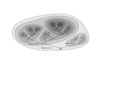
Figure 4: Generic 2D fitness landscape with evolution tree. Each connected slice represents a species. A species is also symbolized by a node in the slice. The number in a slice and near a node is the fitness value of the species. If individuals from one species can evolve to individuals of another species, the nodes are connected by a solid line. Altogether, they form the fitness tree. The branching factor $b$ is $2$ and the number of species per fitness level $s$ is $4$ for intermediate fitness values (3,4,5).

subsectionThe fitness tree model A general, problem independent comparison of the various optimization algorithms is difficult. We are interested in the performance for difficult fitness landscapes with many local optima.

We only consider mutation; recombination is discussed in the next section. The evolutionary neighborhood (not to be confused with $d$-similarity) of an individual $i$ is defined as the set of individuals that can be created from $i$ by a single mutation. Two individuals $i$ and $j$ with the same fitness are defined to belong to the same species if there is a finite sequence of mutations which transforms $i$ into $j$ and all individuals of the sequence also have fitness $f(i)=f(j)$. Each fitness level is partitioned in this way into disjoint species. We say a species of fitness $f+\varepsilon$ can evolve from a species of fitness $f$, if there is a mutation which transforms an individual from the latter species to one of the former. Those species are connected by an edge in Figures 4 and 5. A species is said to be promising if it can evolve to the global optimum $f_{max}$.

8.1 Additional definitions and simplifying assumptions

• Evolution which skips fitness levels is ignored, and also devolution to species of lower fitness other than the primordial species.

• Random individuals have lowest fitness $f_{min}$ with high probability, and there is only one species of fitness $f_{min}$.

• There is a fixed branching factor $b$, i.e. each species can evolve into $b$ improved species, or represents a local optimum from which no further evolution is possible.

• There is a single global optimum $f_{max}$ (or $b$ optima to be consistent with the previous item).

• There are $s$ different species per fitness level (except near $f_{min}$ and $f_{max}$ where there must be fewer to be consistent with the previous items).

• The probability $p$ that an individual evolves to a higher fitness is very small. In most cases a mutation keeps an individual within its species or devolves it.

• The probability to evolve to one of the offspring species is uniform, i.e. $1/b$ for all offspring species.

We have the feeling that this picture covers the essential features of fitness landscapes for difficult problems. The qualitative conclusions we will draw should still hold when some or all of the additional simplifying assumptions are violated.

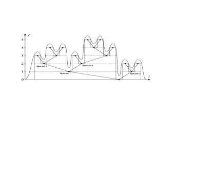
Figure 5: Generic fitness function with evolution tree. Individuals which are evolutionary neighbors are connected by a dashed line. They belong to the species indicated by a node on the dashed line. A species which can evolve from another is connected to it by a solid line. The smooth curve visualizes (somewhat misleading, since the fitness is discrete) the fitness function with many local maxima.

8.2 Example

Consider the case of individuals, which are real-valued $D$ dimensional vectors, i.e. $I={I\mskip-3.0mu\mskip-3.0muR}^{D}$. Let the fitness function $\tilde{f}$ be continuous and positive with many local maxima, which tends to zero for large arguments. This covers a large range of physical optimization problems. Mutation shall be local in ${I\mskip-3.0mu\mskip-3.0muR}^{D}$, i.e. $||i_{original}-i_{mutated}||\ll D$. As FUSS and the fitness tree model is only defined for discrete fitness functions, we discretize $\tilde{f}$ to $f:=\mskip 3.0mu_{\lfloor}{1\over\tilde{\varepsilon}}\tilde{f}_{\rfloor}$, which is acceptable for sufficiently small $\tilde{\varepsilon}$. A typical fitness landscape for $D=2$ and $D=1$ together with their fitness tree are depicted in Figures 4 and 5. Since mutation is a local operation, each species is a (possibly multiply punched) connected slice ($D$-dimensional sub-volume) and evolution can only occur from $f$ to $f+1$ ($\varepsilon=1$). Assumption (i) is generally satisfied. The special fitness landscapes depicted in Figures 4 and 5 also satisfy (ii,iii,iv,v) with $b=2$ and $s=4$.

8.3 Random walk

Consider a mutation induced random walk of a single individual. Due to the low evolution probability $p\ll 1$, most of the time will be spent on individuals of the lowest fitness $f_{min}$. As evolution is a tree, there is only one evolution sequence which leads to the global optimum. At each evolution step, the correct offspring species (out of $b$) has to be evolved. The probability of an evolution step in the right direction, hence, is $p/b$. $|F|$ evolution steps are necessary to reach $f_{max}$. Therefore, the expected time to find the global maximum by random walk is $T_{RW}\approx(b/p)^{|F|}$. Random walk is very slow; it is exponential in the number of fitness levels $|F|$ to a very large basis $b/p$.

8.4 FUSS

Assume that $L$ fitness levels from $f_{min}$ to $f$ are occupied. The probability that FUSS selects an individual of fitness $f$ is $1/L$. Under this additional assumption that the occupation of species within one fitness level is approximately uniform most of the time, the probability of selecting an individual of the promising species, which can evolve to the global optimum, is $1/s$. The probability of an evolution step in the right direction is $p/b$ as in the random walk case. Hence, the total expected time for an evolution in the right direction is $L\cdot s\cdot b/p$. The total time $T_{FUSS}\approx{\textstyle{1\over 2}}|F|^{2}\cdots\cdot b/p$ for an evolution from $L=1$ to the global optimum $L=|F|$ is obtained by summation over $L=1...|F|$.

8.5 FUDS

A similar analysis can be applied to FUDS. Assume again that the $L$ fitness levels from $f_{min}$ to $f$ are occupied and that the occupation of species within each fitness level is approximately uniform most of the time. Because FUDS tends to spread the population out, like FUSS, this assumption is not unreasonable. As FUDS is only a deletion scheme we must also specify a selection scheme. For our analysis we will take a very simple elitist selection scheme that half of the time selects an individual from the highest fitness level, and the other half of the time selects an individual from a lower level. It follows then that the probability of selecting a promising species is $1/2s$ and the probability that this then results in an evolutionary step in the right direction is $p/b$. Thus the total expected time for an evolutionary step in the right direction is $2\cdot s\cdot b/p$. Therefore by summation the total expected time to evolve to the global optimum is $T_{FUDS}\approx 2|F|\cdot s\cdot b/p$. Of course this analysis rests on our choice of selection scheme and the assumptions about the uniformity of the population that we have made. When FUDS is used with selection schemes which are very greedy these uniformity assumptions will likely be violated and less favorable bounds could result.

8.6 Standard selection

We assumed a fixed number of $s$ species per fitness level and $0$ or $b$ offspring species. This implies that only a fraction of $1/b$ species can evolve to higher fitness. We assume that fitness level $f$ has been taken over, i.e. most individuals have fitness $f$. The probability of evolution is $p$. A significant fraction (for simplicity we assume most) of the $|P|$ individuals must evolve to the next fitness level before evolution with a relevant rate can occur to the next to next level. Hence, the time to take over the next fitness level is roughly $|P|\cdot b/p$. As there are $|F|$ fitness levels, the total time is $T_{STD}\mbox{\raisebox{-3.44444pt}{$\stackrel{{\scriptstyle\displaystyle>}}{{\sim}}$}}|F|\cdot|P|\cdot b/p$.

We wrote $\stackrel{{\scriptstyle\displaystyle>}}{{\sim}}$ as we have made two significant favorable assumptions. In order to ensure convergence, the promising species in the current fitness level has to be occupied. If we assume a uniform occupation of species within one fitness level, as for FUSS, this means that all species of the current fitness level have to be populated. As there are $s$ species, $|P|$ has to be at least $s$, which can be quite large. On the other hand, STD linearly slows down with $|P|$, unlike FUSS. Hence, there is a trade-off in the choice of $|P|$.

More serious is the following problem. Assume that the first individual evolved with fitness $f+\varepsilon$ is one in a non-promising species $a$. Due to selection pressure it might happen that species $a$ takes over the whole population before all (or at least the promising) species with fitness $f+\varepsilon$ can evolve from the ones of fitness $f$. The probability to find the global optimum in the worst case scenario, where at each level only one species is occupied, is $(1/b)^{|F|}$. This is the original problem of the loss of genetic diversity discussed at the outset, which lead to the invention of FUSS.

Every other fix the authors are aware of only seems to diminish the problem, but does not solve it. One fix is to repeatedly restart the EA, but the huge number of $b^{|F|}$ restarts might be necessary. The time is exponential in $|F|$ like for random walk but with a smaller basis $b$. The true time is expected to be somewhere in between $|F|\cdot|P|\cdot b/p$ and this worst case analysis, although an unfavorable setting may never reach the global optimum ($T_{STD}=\infty$ in this case).

8.7 Performance comparison

The times $T_{FUSS}$, $T_{FUDS}$ and $T_{STD}$ should be regarded, at best, as rules of thumb, since the derivation was rather heuristic due to the list of assumptions. The quotient is more reliable:

$${T_{FUSS}\over T_{STD}}\quad\mbox{\raisebox{-3.44444pt}{$\stackrel{{\scriptstyle\displaystyle<}}{{\sim}}$}}\quad{|F|\mskip-3.0mu\cdot\mskip-3.0mus\over 2|P|}\quad\mbox{\raisebox{-3.44444pt}{$\stackrel{{\scriptstyle\displaystyle<}}{{\sim}}$}}\quad{\textstyle{1\over 2}}|F|\quad\leq\quad|F|,$$

and

$${T_{FUDS}\over T_{STD}}\quad\approx\quad{\frac{s}{|P|}}\quad\approx\quad 1.$$

We will give a more direct argument in Section 9 that the slowdown of FUSS relative to STD is at most $|F|$.

Finally, a truism has been recovered, namely that an EA can, under certain circumstances, be much faster than random walk, that is, $T_{RW}\gg T_{FUSS},T_{FUDS},T_{STD}$.

9 Scale-Independent Selection and Recombination

9.1 Worst case analysis

We now want to estimate the maximal possible slowdown of FUSS compared to STD. Let us assume that all individuals in STD have fitness $f$, and once one individual with fitness $f+\varepsilon$ has been found, takeover of level $f+\varepsilon$ is quick. Let us assume that this quick takeover is actually good (e.g. if there are no local maxima). The selection probability of individuals of same fitness is equal. For FUSS we assume individuals in the range of $f_{min}$ and $f$. Uniformity is not necessary. In the worst case, a selection of an individual of fitness $<f$ never leads to an individual of fitness $\geq f$, i.e. is always useless. The probability of selecting an individual with fitness $f$ is $\geq{1\over|F|}$. At least every $|F|th$ FUSS selection corresponds to a STD selection. Hence, we expect a maximal slowdown by a factor of $|F|$, since FUSS “simulates” STD statistically every $|F|th$ selection. It is possible to construct problems where this slowdown occurs (unimodal function, local mutation $x\to x\pm\varepsilon$, no crossover). Gradient ascent would be the algorithm of choice in this case. On the other hand, we have not observed this slowdown in our simple 2D example and the TSP experiments, where FUSS outperformed STD in solution quality/time (see the experimental results in Section 12). Since real world problems often lie in between these extreme cases it is desirable to modify FUSS to cope with simple problems as well, without destroying its advantages for complex objective functions.

9.2 Quadratic slowdown due to recombination

We have seen that $T_{FUSS}\leq|F|\cdot T_{STD}$. In the presence of recombination, a pair of individuals has to be selected. The probability that FUSS selects two individuals with fitness $f$ is $\geq{1\over|F|^{2}}$. Hence, in the worst case, there could be a slowdown by a factor of $|F|^{2}$ — for independent selection we expect $T_{FUSS}\leq|F|^{2}\cdot T_{STD}$. This potential quadratic slowdown can be avoided by selecting one fitness value at random, and then two individuals of this single fitness value. For this dependent selection, we expect $T_{FUSS}\leq|F|\cdot T_{STD}$. On the other hand, crossing two individuals of different fitness can also be advantageous, like the crossing of $f=1$ with $f=2$ individuals in the 2D example of Section 7.

9.3 Scale independent selection

A near optimal compromise is possible: a high selection probability $p(f)\sim 1$ if $f\approx f_{max}$ and $p(f)\sim{1\over|F|}$ otherwise. A “scale independent” probability distribution $p(f)\sim{1\over|f_{max}-f|}$ is appropriate for this. We define

$$p(f)\mskip 5.0mu plus 5.0mu:=\mskip 5.0mu plus 5.0mu{c\over\ln|F|}\cdot{1\over{1\over\varepsilon}|f_{max}-f|+1}.$$ (1)

The $+1$ in the denominator has been added to regularize the expression for $f=f_{max}$. The factor $c/\ln|F|$ ensures correct normalization ($\sum_{f}p(f)=1$). By using $\ln{b+1\over a}\leq\sum_{i=a}^{b}{1\over i}\leq\ln{b\over a-1}$, one can show that ${\ln|F|\over 1+\ln|F|}\leq c\leq 1$ i.e. $c\to 1$ for $|F|\to\infty$. In the following we assume $|F|\geq 3$, i.e. $c\geq{\textstyle{1\over 2}}$. Apart from a minor additional logarithmic suppression of order $\ln|F|$ we have the desired behavior $p(f)\sim 1$ for $f\approx f_{max}$ and $p(f)\sim{1\over|F|}$ otherwise:

$$p(f_{max}-m\varepsilon)\geq{1\over 2\ln|F|}\cdot{1\over m+1},$$

$$p(f)\geq{1\over 2\ln|F|}\cdot{1\over|F|}\quad\forall\mskip 3.0muf$$

During optimization, the minimal/maximal fitness of an individual in population $P_{t}$ is $f_{min/max}^{t}$. In the definition of $p$ one has to use $F_{t}:=\{f_{min}^{t},f_{min}^{t}+\varepsilon,...,f_{max}^{t}\}$ instead of $F$, i.e. $|F|$ replaced with $|F_{t}|={1\over\varepsilon}(f_{max}^{t}-f_{min}^{t})+1\leq|F|$. So (1) can not be achieved by a static re-parametrization of fitness $f$ replaced with $g(f)$. Furthermore the important idea of sampling from a fitness level instead of individuals directly is still maintained. The only difference now is that the population will no longer converge to a fitness uniform one but to one with distribution $p(f)$ which is biased toward higher fitness but still never converges to a fittest individual. In the worst case, we expect a small slowdown of the order of $\ln|F|$ as compared to FUSS, as well as compared to STD.

9.4 Scale independent pair selection

It is possible to (nearly) have the best of independent and dependent selection: a high selection probability $p(f,f^{\prime})\sim{1\over|F|}$ if $f\approx f^{\prime}$ and $p(f,f^{\prime})\sim{1\over|F|^{2}}$ otherwise, with uniform marginal $p(f)={1\over|F|}$. The idea is to use a strongly correlated joint distribution for selecting a fitness pair. A “scale independent” probability distribution $p(f,f^{\prime})\sim{1\over|f-f^{\prime}|}$ is appropriate. We define the joint probability $\tilde{p}(f,f^{\prime})$ of selecting two individuals of fitness $f$ and $f^{\prime}$ and the marginal $\tilde{p}(f)$ as

$$\tilde{p}(f,f^{\prime})\mskip 5.0mu plus 5.0mu:=\mskip 5.0mu plus 5.0mu{1\over 2|F|\ln|F|}\cdot{1\over{1\over\varepsilon}|f\mskip-3.0mu-\mskip-3.0muf^{\prime}|+1},$$ (2)

$$\tilde{p}(f)\mskip 5.0mu plus 5.0mu:=\mskip 5.0mu plus 5.0mu\sum_{f^{\prime}\in F}\tilde{p}(f,f^{\prime})=\sum_{f^{\prime}\in F}\tilde{p}(f^{\prime},f).$$

We assume $|F|\geq 3$ in the following. The $+1$ in the denominator has been added to regularize the expression for $f=f^{\prime}$. The factor $(2|F|\ln|F|)^{-1}$ ensures correct normalization for $|F|\to\infty$. More precisely, using $\ln{b+1\over a}\leq\sum_{i=a}^{b}{1\over i}\leq\ln{b\over a-1}$, one can show that

$$1-{\textstyle{1\over\ln|F|}}\mskip 5.0mu plus 5.0mu\leq\mskip 5.0mu plus 5.0mu\sum_{f,f^{\prime}\in F}\tilde{p}(f,f^{\prime})\mskip 5.0mu plus 5.0mu\leq\mskip 5.0mu plus 5.0mu1,\quad{\textstyle{1\over 2}}\mskip 5.0mu plus 5.0mu\leq\mskip 5.0mu plus 5.0mu|F|\mskip-3.0mu\cdot\mskip-3.0mu\tilde{p}(f)\mskip 5.0mu plus 5.0mu\leq\mskip 5.0mu plus 5.0mu1,$$

i.e. $\tilde{p}$ is not strictly normalized to $1$ and the marginal $\tilde{p}(f)$ is only approximately (within a factor of 2) uniform. The first defect can be corrected by appropriately increasing the diagonal probabilities $\tilde{p}(f,f)$. This also solves the second problem.

$$p(f,f^{\prime})\mskip 5.0mu plus 5.0mu:=\mskip 5.0mu plus 5.0mu\left\{\begin{array}[]{ll}\tilde{p}(f,f^{\prime})&\mbox{for}\quad f\neq f^{\prime}\\ \tilde{p}(f,f^{\prime})+[{1\over|F|}-\tilde{p}(f)]&\mbox{for}\quad f=f^{\prime}\end{array}\right.$$ (3)

9.5 Properties of $p(f,f^{\prime})$

$p$ is normalized to $1$ with uniform marginal

$$p(f):=\sum_{f^{\prime}\in F}p(f,f^{\prime})={1\over|F|},$$

$$\sum_{f,f^{\prime}\in F}p(f,f^{\prime})=\sum_{f\in F}p(f)=1,$$

$$p(f,f^{\prime})\geq\tilde{p}(f,f^{\prime}).$$

Apart from a minor additional logarithmic suppression of order $\ln|F|$ we have the desired behavior $p(f,f^{\prime})\sim{1\over|F|}$ for $f\approx f^{\prime}$ and $p(f,f^{\prime})\sim{1\over|F|^{2}}$ otherwise:

$$p(f,f\pm m\varepsilon)\geq{1\over 2\ln|F|}\cdot{1\over m+1}\cdot{1\over|F|},$$

$$p(f,f^{\prime})\geq{1\over 2\ln|F|}\cdot{1\over|F|^{2}}.$$

During optimization, the minimal/maximal fitness of an individual in population $P_{t}$ is $f_{min/max}^{t}$. In the definition of $p$ one has to use $F_{t}:=\{f_{min}^{t},f_{min}^{t}+\varepsilon,...,f_{max}^{t}\}$ instead of $F$, i.e. $|F|$ replaced with $L:=|F_{t}|={1\over\varepsilon}(f_{max}^{t}-f_{min}^{t})+1\leq|F|$.

9.6 Scale-Independent Deletion

Just as the selection scheme FUSS has its dual in the deletion scheme FUDS, we can likewise create the dual of Scale-Independent Selection in the form of Scale-Independent Deletion. Thus rather than targeting deletion from the population so that the distribution becomes flat, as we do with FUDS, we now define a convex curve $g$ which is peaked at the fittest individual in the population and delete the population down so that it follows the shape of this curve. This retains some of the advantages of FUDS, for example the population cannot collapse to just a few fitness levels, and yet it recognizes that for many problems it is useful to bias the population distribution toward fit individuals. Of course such problems are less deceptive than the kind that FUSS and FUDS are intended for.

10 Continuous Fitness Functions

10.1 Effective discretization scale

Up to now we have considered a discrete valued fitness function with values in $F=\{f_{min},f_{min}+\varepsilon,...,f_{max}\}$. In many practical problems, the fitness function is continuous valued with $F=[f_{min},f_{max}]$. We generalize FUSS, and some of the discussion of the previous sections to the continuous case by replacing the discretization scale $\varepsilon$ by an effective (time-dependent) discretization scale $\hat{\varepsilon}$. By construction, FUSS shifts the population toward a more uniform one. Although the fitness values are no longer equi-spaced, they still form a discrete set for finite population $P$. For a fitness uniform distribution, the average distance between (fitness) neighboring individuals is ${1\over|P_{t}|-1}(f^{t}_{max}-f^{t}_{min})=:\hat{\varepsilon}$. We define $\hat{F}_{t}:=\{f^{t}_{min},f^{t}_{min}+\hat{\varepsilon},...,f^{t}_{max}\}$. $|\hat{F}_{t}|={1\over\hat{\varepsilon}}(f^{t}_{max}-f^{t}_{min})+1=|P_{t}|$.

10.2 FUSS

Fitness uniform selection for a continuous valued function has already been mentioned in Section 3. We just take a uniform random fitness $f$ in the interval $[f_{min}^{t}-{\textstyle{1\over 2}}\hat{\varepsilon},f_{max}^{t}+{\textstyle{1\over 2}}\hat{\varepsilon}]$. Independent and dependent fitness pair selection as described in the last section works analogously. An $\hat{\varepsilon}=0$ version of correlated selection does not exist; a non-zero $\hat{\varepsilon}$ is important. A discrete pair $(f,f^{\prime})$ is drawn with probability $p(f,f^{\prime})$ as defined in (2) and (3) with $\varepsilon$ and $F$ replaced by $\hat{\varepsilon}$ and $\hat{F}_{t}$. The additional suppression $\ln|\hat{F}|=\ln|P_{t}|$ is small for all practically realizable population sizes. In all cases an individual with fitness nearest to $f$ ($f^{\prime}$) is selected from the population $P$ (randomly if there is more than one nearest individual).

If we assume a fitness uniform distribution then our worst case bound of $T_{FUSS}\mbox{\raisebox{-3.44444pt}{$\stackrel{{\scriptstyle\displaystyle<}}{{\sim}}$}}\sum_{t=1}^{T_{STD}}|P_{t}|$ is plausible, since the probability of selecting the best individual is approximately $|P_{t}|$. For constant population size we get a bound $T_{FUSS}\mbox{\raisebox{-3.44444pt}{$\stackrel{{\scriptstyle\displaystyle<}}{{\sim}}$}}|P|\cdot T_{STD}$. For the preferred non-deletion case with population size $|P_{t}|=t$ the bound gets much worse $T_{FUSS}\mbox{\raisebox{-3.44444pt}{$\stackrel{{\scriptstyle\displaystyle<}}{{\sim}}$}}{\textstyle{1\over 2}}T_{STD}^{2}$. This possible (but not necessary!) slowdown has similarities to the slowdown problems of proportionate selection in later optimization stages. The species definition in Section 8 has to be relaxed by allowing mutation sequences of individuals with $\hat{\varepsilon}$-similar fitness. Larger choices of $\hat{\varepsilon}$ may be favorable if the standard choice causes problems.

10.3 FUDS

Fitness uniform deletion already requires the range of the fitness function to be broken up into a finite number of intervals. While for discrete valued fitness functions the intervals may correspond to the unique values of the fitness function, this is not a requirement. Indeed if the population is small and the fitness function has a large number of possible values then a more coarse discretization is necessary. Continuous valued fitness functions can therefore be treated in exactly the same way and do not cause any special problems. In fact they are slightly simpler in that we are now free to choose the discretization as fine as we like without being limited by the number of possible fitness values. Of course, like in the discrete case, we still must choose a discretization which is appropriate given the size of the population.

11 The EA Test System

To test FUSS and FUDS we have implemented an EA test system in Java. The complete source code along with the test problems presented in this paper and basic usage instructions can be downloaded from [Leg04]. The EA model we have chosen for our tests is the so called “steady state” model as opposed to the more usual “generational” model. In a generational EA in each generation we select an entirely new population based on the old population. The old population is then simply discarded. Under the steady state model that we use, each step of the optimization adds and removes just one individual at a time. Specifically the process occurs as follows: Firstly an individual is selected by the selection scheme and then with a certain probability another individual is also selected and the crossover operator is applied to produce a new individual. Then with another probability a mutation operator is applied to produce the child individual which is then added to the population. We refer to the probability of crossing as the crossover probability and the probability of mutating following a crossover as the mutation probability. In the case where no crossover takes place the individual is always mutated to ensure that we are not simply adding a clone of an existing individual into the population. Finally, an individual must be deleted in order to keep the population size constant. This individual is selected by the deletion scheme. The deletion scheme is important as it has the power to bias the population in a similar way to the selection scheme.

Our task in this paper is to experimentally analyze how FUSS performs relative to other selection schemes and how FUDS performs relative to other deletion schemes. Because any particular run of a steady state EA requires both a selection and a deletion scheme to be used, there are many possible combinations that we could test. We have narrowed this range of possibilities down to just a few that are commonly used.

Among the selection schemes, tournament selection is one of the simplest and most commonly used and we consider it to be roughly representative of other standard selection schemes which favor the fitter individuals in the population; indeed in the case of tournament size 2 it can be shown that tournament selection is equivalent to the linear ranking selection scheme [Hut91, Sec.2.2.4]. With tournament selection we randomly pick a group of individuals and then select the fittest individual from this group. The size of the group is called the tournament size and it is clear that the larger this group is the more likely we are to select a highly fit individual from the population. At some point in the future we may implement other standard selection schemes to broaden our comparison, however we expect the performance of these schemes to be at best comparable to tournament selection when used with a correctly tuned selection intensity.

Among the deletion schemes one of the most commonly used in steady state EAs is random deletion. The rational for this is that it is neutral in the sense that it does not skew the distribution of the population in any way. Thus whether the population tends toward high or low fitness etc. is solely a function of the selection scheme and its settings. Of course random deletion, unlike FUDS, makes no effort to preserve diversity in the population as all individuals have an equal chance of being removed. In this paper we will compare FUDS against random deletion as this is the standard deletion schemes in situations where it is difficult or impossible to directly measure the similarity of individuals based on their genomes.

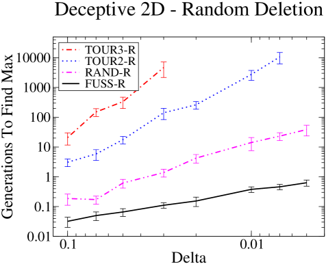
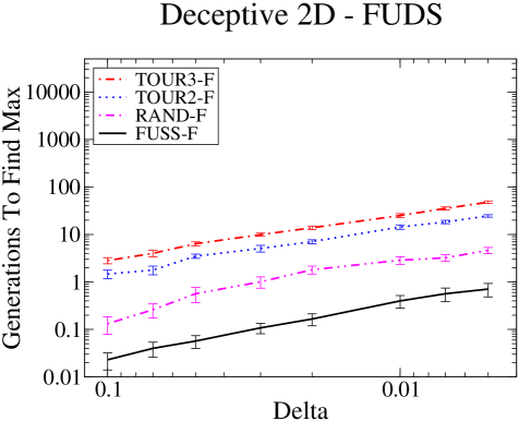
Figure 6: With random deletion (left graph) FUSS significantly outperforms TOURx and RAND. By switching to FUDS (right graph) the performance of TOURx and RAND now scale the same as FUSS.

When reporting test results we will adopt the following notation: TOUR2 means tournament selection with a tournament size of 2. Similarly for TOUR3, TOUR4 and so on. Under random selection, denoted RAND, all members of the population have an equal probability of being selected. This is sometimes called uniform selection. When a graph shows the performance of tournament selection over a range of tournament sizes we will simply write TOURx. Naturally FUSS indicates the fitness uniform selection scheme. To indicate the deletion scheme used we will add either the suffix -R or -F to indicate random deletion or FUDS respectively. Thus, TOUR10-R is tournament selection with a tournament size of 10 used with random deletion, while FUSS-F is FUSS selection used with FUDS deletion.

The important free parameters to set for each test are the population size, and the crossover and mutation probabilities. Good values for the crossover and mutation probabilities depend on the problem and must be manually tuned based on experience as there are few theoretical guidelines on how to do this. For some problems performance can be quite sensitive to these values while for others they are less important. Our default values are 0.5 for both as this has often provided us with reasonable performance in the past.

For each test we ran the system multiple times with the same mutation and crossover probabilities and the same population size. The only difference was which selection and deletion schemes were used by the code. Thus even if our various parameters, mutation operators etc. were not optimal for a given problem, the comparison is still fair. Indeed we often deliberately set the optimization parameters to non-optimal values in order to compare the robustness of the systems.

As a steady state optimizer operates on just one individual at a time, the number of cycles within a given run can be high, perhaps 100,000 or more. In order to make our results more comparable to a generational optimizer we divide this number by the size of the population to give the approximate number of generations. Unfortunately the theoretical understanding of the relationship between steady state and generational optimizers is not strong. It has been shown that under the assumption of no crossover the effective selection intensity using tournament selection with size 2 is approximately twice as strong under a steady state EA as it is with a generational EA [RPB99b]. As far as we are aware a similar comparison for systems with crossover has not been performed.

Depending on the purpose of a test run, different stopping criteria were applied. For example, in situations where we wanted to graph how rapidly different strategies converged with respect to generations, it made sense to fix the number of generations. In other situations we wanted to stop a run once the optimizer appeared to have become stuck, that is, when the maximum fitness had not improved after some specified number of generations. In any case we explain for each test the stopping criterion that has been used.

In order to generate reliable statistics we ran each test multiple times; typically 30 times but sometimes up to 100 times if the results were noisy. From these runs we then calculated the mean performance as well as the sample standard deviation and from this the standard error in our estimate of the mean. This value was then used to generate the 95% confidence intervals which appear as error bars on the graphs.

12 A Deceptive 2D Problem

The first problem we examine is the simple but highly deceptive 2D optimization problem which was theoretically analyzed in Section 7. As in the theoretical analysis, we set up the mutation operator to randomly replace either the $x$ or $y$ position of an individual and the crossover to take the $x$ position from one individual and the $y$ position from another to produce an offspring. The size of the domain for which the function is maximized is just $\delta^{2}$ which is very small for small values of $\delta$, while the local maxima at fitness level 3 covers most of the space. Clearly the only way to reach the global maximum is by leaving this local maximum and exploring the space of individuals with lower fitness values of 1 or 2. Thus, with respect to the mutation and crossover operators we have defined, this is a deceptive optimization problem as these partitions mislead the EA [FM93].

For this test we set the maximum population size to 1,000 and made 20 runs for each $\delta$ value. With a steady state EA it is usual to start with a full population of random individuals. However for this particular problem we reduced the initial population size down to just 10 in order to avoid the effect of doing a large random search when we created the initial population and thereby distorting the scaling. Usually this might create difficulties due to the poor genetic diversity in the initial population. However due to the fact that any individual can mutate to any other in just two steps this is not a problem in this situation. Initial tests indicated that reducing the crossover probability from 0.5 to 0.25 improved the performance slightly and so we have used the latter value.

The first set of results for the selection schemes used with random deletion appear in the left graph of Figure 6. As expected, higher selection intensity is a significant disadvantage for this problem. Indeed even with just a tournament size of 3 the number of generations required to find the maximum became infeasible to compute for smaller values of $\delta$. Our results confirm the theoretical scaling orders of $1\over\delta^{2}$ for TOUR2-R, and $1\over\delta$ for FUSS-R, as predicted in Section 7. Be aware that this is a log-log scaled graph and so the different slopes indicate significantly different orders of scaling.

In the second set of tests we switch from random deletion to FUDS. These results appear in the right graph of Figure 6. We see that with FUDS as the deletion scheme the scaling improves dramatically for RAND, TOUR2 and TOUR3. Indeed they are now of the same order $\frac{1}{\delta}$ as FUSS, as predicted in Section 7. This shows that for very deceptive problems much higher levels of selection intensity can be applied when using FUDS rather than random deletion. The performance of FUSS-R is very similar to that of FUSS-F. This is not surprising as the population distribution under FUSS already tends to be approximately uniform across fitness levels and thus we expect the effect of FUDS to be quite weak.

Although this problem was artificially constructed, the results clearly demonstrate how FUSS and FUDS can dramatically improve performance in some situations.

13 Traveling Salesman Problem

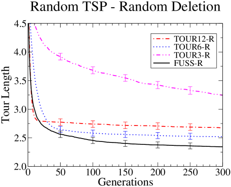
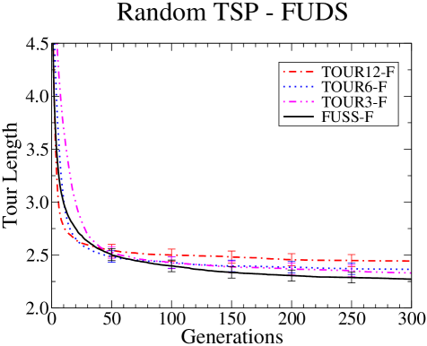
Figure 7: TOUR3-R converged too slowly while TOUR12-R converged prematurely and became stuck. TOUR6-R appears to be about the correct tournament size for this problem, however it is still inferior to FUSS-R. With FUDS all of the selection schemes performed well though FUSS was still the best.

A well known optimization problem is the so called Traveling Salesman Problem (TSP). The task is to find the shortest Hamiltonian cycle (path) in a graph of $N$ vertexes (cities) connected by edges of certain lengths. There exist highly specialized population based optimizers which use advanced mutation and crossover operators and are capable of finding paths less than one percent longer than the optimal path for up to $10^{7}$ cities [LK73, MO96, JM97, ACR00]. As our goal is only to study the relative performance of selection and deletion schemes, having a highly refined implementation is not important. Thus the mutation and crossover operators we used were quite simple: Mutation was achieved by just switching the position of two of the cities in the solution, while for crossover we used the partial mapped crossover technique [GA85]. Fitness was computed by taking the reciprocal of the tour length.

For our first set of tests we used randomly generated TSP problems, that is, the distance between any two cities was chosen uniformly from the unit interval $[0,1]$. We chose this as it is known to be a particularly deceptive form of the TSP problem as the usual triangle inequality relation does not hold in general. For example, the distance between cities $A$ and $B$ might be $0.1$, between cities $B$ and $C$ $0.2$, and yet the distance between $A$ and $C$ might be $0.8$. The problem still has some structure though as efficient partial solutions tend to be useful building blocks for efficient complete tours.

For this test we used random distance TSP problems with 20 cities and a population size of 1000. We found that changing the crossover and mutation probabilities did not improve performance and so these have been left at their default values of 0.5. Our stopping criterion was simply to let the EA run for 300 generations as this appeared to be adequate for all of the methods to converge and allowed us to easily graph performance versus generations.

The first graph in Figure 7 shows each of the selection schemes used with random deletion. We see that TOUR3-R has insufficient selection intensity for adequate convergence while TOUR12-R quickly converges to a local optimum and then becomes stuck. TOUR6-R has about the correct level of selection intensity for this problem and population size. FUSS-R however initially converges as rapidly as TOUR12-R but avoids becoming stuck in local optima. This suggests improved population diversity. The performance curve for FUSS-R is impressive, especially considering that it is parameterless.

At first it might seem surprising that the maximum fitness with FUSS climbs very quickly for the first 20 generations, especially considering that FUSS makes no attempt to increase the average fitness in the population. However we can explain this very rapid rise in solution fitness by considering a simple example. Consider a situation where there is a large number of individuals in a small band of fitness levels, say 1,000 with fitness values ranging from 50 to 70. Add to this population one individual with a fitness value of 73. Thus the total fitness range contains 24 values. Whenever FUSS picks a random point from 72 to 73 inclusive this single individual with maximal fitness will be selected. That is, the probability that the single fittest individual will be selected is 2/24 = 0.083. In comparison under TOUR12 the probability that the fittest individual is selected is the same as the probability that it is picked for the sample of 12 elements used for the tournament, which is approximately, 12/1000 = 0.012. Thus the probability of the fittest individual in the population being selected is higher under FUSS than under TOUR12 and so the maximum fitness would rise quickly to start with.

Previously in [LHK04] we speculated that this may have been responsible for performance problems that we had observed with FUSS in some situations. However further experimentation has shown that very rapid rises in maximal fitness are quite rare and are also very shortly lived when they do occur — too short to cause any significant diversity problems in the population. We now believe that the population distribution is to blame in these situations; something that we will explore in detail in Section 15.

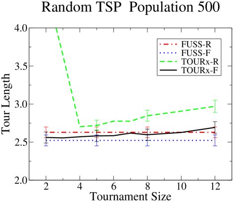
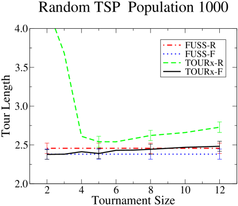
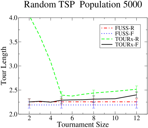
Figure 8: The performance of TOURx-F is much more stable than TOURx-R under variation in the selection intensity. Also both FUSS-R and FUSS-F produce very good results, especially with the larger populations.

The second graph in Figure 7 shows the same set of selection schemes but now using FUDS as the deletion scheme. With FUDS the performance of all of the selection schemes either stayed the same or improved. In the case of TOUR3 the improvement was dramatic and for TOUR12 the improvement was also quite significant. This is interesting because it shows that with fitness uniform deletion, performance can improve when the selection intensity is either too high or too low. That is, when using FUDS the performance of the EA now appears to be more robust with respect to variation in selection intensity.

In the case of TOUR12-F this is evidence of improved population diversity as the EA is no longer becoming stuck. However for TOUR3-R the selection intensity is quite low and thus we would expect the population diversity to be relatively good. Thus the fact that TOUR3-F was so much better than TOUR3-R suggests that FUDS can have significant performance benefits that are not related to improved population diversity.

Investigating further it seems that this effect is due to the way that FUDS focuses the deletion on the large mass of individuals which have an average level of fitness while completely leaving the less common fit individuals alone. This helps a system with very weak selection intensity move the mass of the population up through the fitness space. With higher selection intensity this problem tends not to occur as individuals in this central mass are less likely to be selected thus reducing the rate at which new individuals of average fitness are added to the population.

In order to better understand how stable FUDS performance is when used with different selection intensities we ran another set of tests on random TSP problems with 20 cities and graphed how performance varied by tournament size. For these tests we set the EA to stop each run when no improvement had occurred in 40 generations. We also tested on a range of population sizes: 250, 500, 1000 and 5000. The results appear in Figure 8.

In these graphs we can now clearly see how the performance of TOURx-R varies significantly with tournament size. Below the optimal tournament size performance worsened quickly while above this value it also worsened, though more slowly. Interestingly, with a population size of 5000 the optimal tournament size was about 6, while with small populations the optimal value fell to just 4. Presumably this was partly because smaller populations have lower diversity and thus cannot withstand as much selection intensity.

In contrast FUSS-R and FUSS-F appear as horizontal lines as they do not have a tournament size parameter. We see that they have performed as well as the optimal performance of TOURx-R without requiring any tuning. Indeed for larger populations FUSS-R appears to be even better than the optimally tuned performance of TOURx-R. This is a very positive result for the parameterless FUSS.

Comparing FUDS with random deletion we also see impressive results. For every combination of selection scheme, tournament size and population size the result with FUDS was better than the corresponding result with random deletion, and in some cases much better. Furthermore these graphs clearly display the improved robustness of tournament selection with FUDS as TOURx-F produced near optimal results for all tournament sizes. Even with an optimally tuned tournament size FUDS increased performance, particularly with the smaller populations. Indeed for each population size tested the worst performance of TOURx-F was equal to the best performance of TOURx-R.

With FUSS there was also a performance advantage when using FUDS, again more so with the smaller populations. The combination of both FUSS and FUDS was especially effective as can be seen by the consistently superior performance of FUSS-F across all of the graphs.

More tests were run exploring performance with up to 100 cities. Although the performance of FUDS remained stronger than random deletion for very low selection intensity, for high selection intensity the two were equal. We believe that the reason for this is the following: When the space of potential solutions is very large finding anything close to a global optimum is practically impossible, indeed it is difficult to even find the top of a reasonable local optimum as the space has so many dimensions. In these situations it is more important to put effort into simply climbing in the space rather than spreading out and trying to thoroughly explore. Thus higher selection intensity can be an advantage for large problem spaces. At any rate, for large problems and with high selection intensity FUDS did not appear to hinder the performance, while with low selection intensity it continued to significantly improve it.

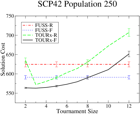
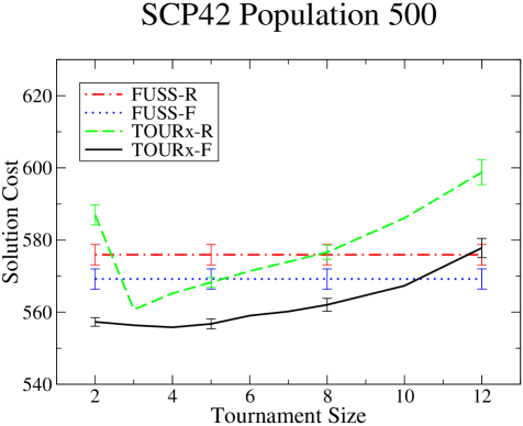
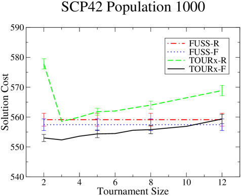
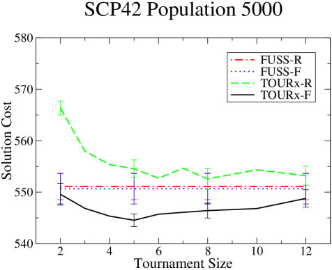
Figure 9: The performance of FUSS for the two smaller populations was relatively poor, while for the larger populations it matched the optimal performance of TOURx-R. FUDS again produced superior results to random deletion in all situations tested.

Experiments were also performed using the more efficient “2-Opt” mutation operator. As expected, this increased performance and allowed much higher selection pressure to be used. Of course the problem then no longer had the kind of deceptive structure that heavily punishes high selection pressure that we are looking for. Nevertheless, FUDS continued to significantly boost the performance of tournament selection, in particular when the tournament size was too small.

14 Set Covering Problem

The set covering problem (SCP) is a reasonably well known NP-complete optimization problem with many real world applications. Let $M\in\{0,1\}^{m\times n}$ be a binary valued matrix and let $c_{j}>0$ for $j\in\{1,\ldots n\}$ be the cost of column $j$. The goal is to find a subset of the columns such that the cost is minimized. Define $x_{j}=1$ if column $j$ is in our solution and 0 otherwise. We can then express the cost of this solution as $\sum_{j=1}^{n}c_{j}x_{j}$ subject to the condition that $\sum_{j=1}^{n}m_{ij}x_{j}\geq 1$ for $i\in\{1,\ldots m\}$.

Our system of representation, mutation operators and crossover follow that used by Beasley [BC96] and we compute the fitness by taking the reciprocal of the cost. The results presented here are based on the “scp42” problem from a standard collection of SCP problems [Bea03]. The results obtained on other problems in this test set were similar. We found that increasing the crossover probability and reducing the mutation probability improved performance, especially when the selection intensity was low. Thus we have tested the system with a crossover probability of 0.8 and a mutation probability of 0.2. We performed each test at least 50 times in order to minimize the error bars. Our stopping criterion was to terminate each run after no improvement in minimal cost had occurred for 40 generations. The results for this test appear in Figure 9.

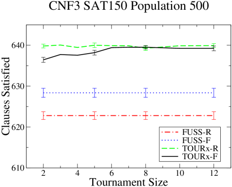
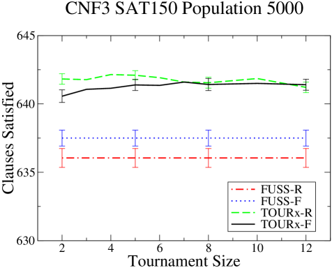
Figure 10: With low selection intensity TOURx-F performed slightly below TOURx-R, but was otherwise comparable. FUSS had serious difficulties.

Similar to the TSP graphs we again see the importance of correctly tuning the tournament size with TOURx-R. We also see the optimal range of performance for TOURx-R moving to the right as the population sizes increases. This is what we would expect due to the greater diversity in larger populations. This kind of variability is one of the reasons why the selection intensity parameter usually has to be determined by experimentation.

Unlike with TSP however, the performance of FUSS was less convincing in these results. With the smaller populations of 250 and 500 FUSS-R was only better than TOURx-R when the tournament size was very low or very high. With the larger populations of 1,000 and 5,000 the results were much better with FUSS-R performing as well as the optimal performance of TOURx-R. FUSS-F performed better than FUSS-R, in particular with the smaller populations though this improvement was still insufficient for it to match the optimal performance of TOURx-R in these cases. The fact that the performance of FUSS varied by population size suggests that FUSS might be experiencing some kind of population diversity problem. We will look more carefully at diversity issues in the next section.

With FUDS the results were again very impressive. As with the TSP tests; for all combinations of selection scheme, tournament size and population size that we tested, the performance with FUDS was superior to the corresponding performance with random deletion. This was true even when the tournament size was optimal. While the performance of TOURx-F did vary significantly with different tournament sizes, the results were more robust than TOURx-R, especially with the larger populations. Indeed for the larger two populations we again have a situation where the worst performance of TOURx-F is equal to the optimal performance of TOURx-R.

15 Maximum CNF3 SAT

Maximum CNF3 SAT is a well known NP hard optimization problem [CK03] that has been extensively studied. A three literal conjunctive normal form (CNF) logical equation is a boolean equation that consists of a conjunction of clauses where each clause contains a disjunction of three literals. So for example, $(a\lor b\lor\lnot c)\land(a\lor\lnot e\lor f)$ is a CNF3 expression. The goal in the maximum CNF3 SAT problem is to find an instantiation of the variables such that the maximum number of clauses evaluate to true. Thus for the above equation if $a=F$, $b=T$, $c=T$, $e=T$, and $f=F$ then just one clause evaluates to true and thus this instantiation gets a score of one. Achieving significant results in this area would be difficult and this is not our aim; we are simply using this problem as a test to compare selection and deletion schemes.

Our test problems have been taken from the SATLIB collection of SAT benchmark tests [HS00]. The first test was performed on the full set of 100 instances of randomly generated CNF3 formula with 150 variables and 645 clauses, all of which are known to be satisfiable. Based on test results the crossover and mutation probabilities were left at the default values. Our mutation operator simply flips one boolean variable and the crossover operator forms a new individual by randomly selecting for each variable which parent’s state to take. Fitness was simply taken to be the number of classes satisfied. Again we tested across a range of tournament sizes and population sizes. The results of these tests appear in Figure 10.

We have shown only the population sizes of 500 and 5,000 as the other population sizes tested followed the same pattern. Interestingly for this problem there was no evidence of better performance with FUDS at higher selection intensities. Nor for that matter was there the decline in performance with TOURx-R that we have seen elsewhere. Indeed with random deletion the selection intensity appeared to have no impact on performance at all. While SAT3 CNF is an NP hard optimization problem, this lack of dependence of our selection intensity parameter suggests that it may not have the deceptive structure that FUSS and FUDS are designed for.

With low selection intensity FUDS caused performance to fall below that of random deletion; something that we have not seen before. Because the advantages of FUDS have been more apparent with low populations in other test problems, we also tested the system with a population size of only 150. Unfortunately no interesting changes in behavior were observed.

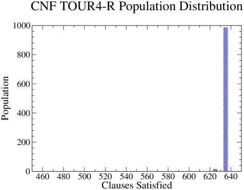
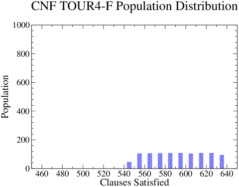
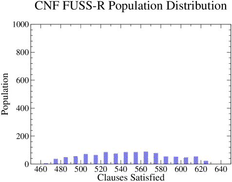
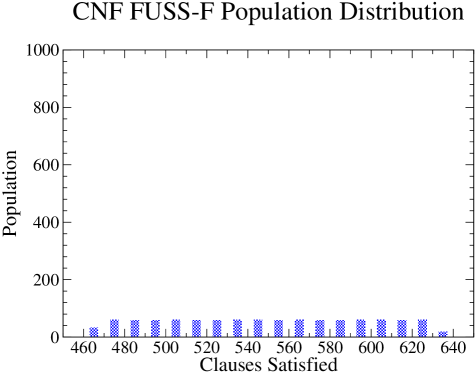
Figure 11: With TOUR4-R the population collapses to a narrow band of fitness levels while with TOUR4-F the distribution is flat. Under FUSS the population spreads out in both directions with FUSS-F in particular giving an extremely uniform distribution.

While FUDS had minor difficulties, FUSS had serious problems for all the population sizes that we tested. We suspected that the uniform nature of the population distribution that should occur with both FUSS and FUDS might be to blame as we only expect this to be a benefit for very deceptive problems which are sensitive to the tuning of the selection intensity parameter. Thus we ran the EA with a population of 1000 and graphed the population distribution across the number of clauses satisfied at the end of the run. We stopped each run when the EA made no progress in 40 generations. The results of this appear in Figure 11.

The first thing to note is that with TOUR4-R the population collapses to a narrow band of fitness levels, as expected. With TOUR4-F the distribution is now uniform, though practically none of the population satisfies fewer than 550 clauses. The reason for this is quite simple: While FUDS levels the population distribution out, TOUR4 tends to select the most fit individuals and thus pushes the population to the right from its starting point. In contrast, FUSS pushes the population toward currently unoccupied fitness levels. This results in the population spreading out in both directions and so the number of individuals with extremely poor fitness is much higher.

Given that our goal is to find an instantiation that satisfies all 645 clauses, it is questionable whether having a large percentage of the population unable to satisfy even 600 clauses is of much benefit. While the total population diversity under FUSS-F might be very high, perhaps the kind of diversity that matters the most is the diversity among the relatively fit individuals in the population. This should be true for all but the most excessively deceptive problems. By thinly spreading the population across a very wide range of fitness levels we actually end up with very few individuals with the kind of diversity that matters. Of course this depends on the nature of the problem we are trying to solve and the fitness function that we use.

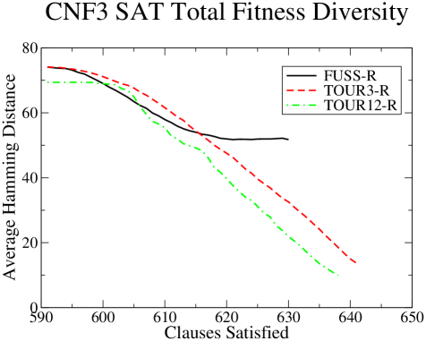
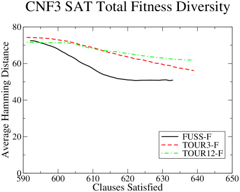
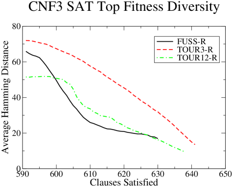
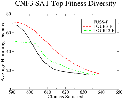
Figure 12: While the total population diversity is very strong under FUSS, the diversity among fit individuals is weak. FUDS improves the total population diversity compared to random deletion, but has little effect on the diversity among the fit individuals.

Fortunately with CNF3 SAT we can directly measure population diversity by taking the average hamming distance between individuals’ genomes. While this means that the value of the fitness based similarity metric is questionable for this problem, as more direct methods like crowding can be applied, it is a useful situation for our analysis as it allows us to directly measure how effective FUSS and FUDS are at preserving population diversity. The hope of course is that any positive benefits that we have seen here will also carry over to problems where directly measuring the diversity is problematic.

For the diversity tests we used a population size of 1000 again. For comparison we used FUSS, TOUR3 and TOUR12 both with random deletion and with FUDS. In each run we calculated two different statistics: The average hamming distance between individuals in the whole population, and the average hamming distance between individuals whose fitness was no more than 20 below the fittest individual in the population at the time. These two measurements give us the “total population diversity” and “high fitness diversity” graphs in Figure 12.

We graphed these measurements against the solution cost of the fittest individual rather than the number of generations. This is only fair because if good solutions are found very quickly then an equally rapid decline in diversity is acceptable and to be expected. Indeed it is trivial to come up with a system which always maintains high population diversity how ever long it runs, but is unlikely to find any good solutions. The results were averaged over all 100 problems in the test set. Because the best solution found in each run varied we have only graphed each curve until such a point where fewer than 50% of the runs were able to achieve this level of fitness. Thus the terminal point at the right of each curve is representative of fairly typical runs rather than just a few exceptional ones that perhaps found unusually good solutions by chance.

The top two graphs in Figure 12 show the total population diversity. As expected the diversity with TOUR3-R and TOUR12-R decline steadily as finding better solutions becomes increasingly difficult and the population tends to collapse into a narrow band of fitness. As we would expect, the total population diversity with TOUR3-R is higher than with TOUR12-R. While FUSS-R declines initially it then stabilizes at around 50 before becoming stuck. As the TOUR3-R and TOUR12-R curves both extend further to the right, even though the total population diversity becomes quite low, this show that diversity problems in the population as a whole are not a significant factor behind the performance problems with FUSS-R.

The top right graph shows the same selection schemes, but this time with FUDS. As expected FUDS has significantly improved the total population diversity with both TOUR3 and TOUR12, while having little impact on FUSS which already has a relatively flat population distribution. As the maximal solution found by TOUR3-F and TOUR12-F were not better than TOUR3-R and TOUR12-R, this indicates that improved total population diversity is not a significant factor in the performance of the EA for this type of optimization problem. That FUDS has lifted the total diversity for TOUR3 and TOUR12 so that they are now above FUSS-F, is particularly interesting. This suggests that while FUSS has high total population diversity, there appears to be some more subtle effects that are causing the diversity to be lower than it could be. It may be related to the fact the FUSS sometimes heavily selects from small groups within the population during the early stages of the optimization process, as we noted in Section 13. However we are not certain whether this is occurring in this case.

On the lower set of graphs we see the diversity among the fitter individuals in the population; specifically those whose fitness is no more than 20 below the fittest individual in the population at the time. On the first graph on the left we see that TOUR3 has significantly greater diversity than TOUR12 with both deletion schemes. This is expected as TOUR3 tends to search more evolutionary paths while TOUR12 just rushes down a few. Disappointingly FUDS does not appear to have made much difference to the diversity among these highly fit individuals, though the curves do flatten out a little as the diversity drops below 30, so perhaps FUDS is having a slight impact.

For both FUSS-R and FUSS-F the diversity among the fit individuals was poor, indeed it was even worse than TOUR12 for both deletion schemes. Thus, while the total population diversity with FUSS tends to be high, the diversity among the fittest individuals in the population can be quite poor. Furthermore, the curves for high fitness diversity all end once the diversity drops into the 12 to 17 range. As this pattern was absent from the graphs of total population diversity, this indicates that it is indeed the diversity among the relatively fit individuals in the population that most determines when the EA is going to become stuck.

In summary, these results show that while FUSS has been successful in maximizing total population diversity, for problems such as CNF3 SAT this is not sufficient. It appears to be more important that the EA maximizes the diversity among those individuals which have higher fitness and in this regard FUSS is poor, which leads to poor performance. This is most likely a characteristic of optimization problems which, while still difficult, are not as deceptive as SCP or random TSP.

16 Conclusions and Future Research Directions

We have addressed the problem of balancing the selection intensity in EAs, which determines speed versus quality of a solution. We invented a new fitness uniform selection scheme FUSS. It generates a selection pressure toward sparsely populated fitness levels. This property is unique to FUSS as compared to other selection schemes (STD). It results in the desired high selection pressure toward higher fitness if there are only a few fit individuals. The selection pressure is automatically reduced when the number of fit individuals increases. We motivated FUSS as a scheme which bounds the number of similar individuals in a population. We defined a universal similarity relation solely depending on the fitness, independent of the problem structure, representation and EA details. We showed analytically by way of a simple example that FUSS can be much more effective than STD. A joint pair selection scheme for recombination has been defined. A heuristic worst case analysis of FUSS compared to STD has been given. For this, the fitness tree model has been defined, which is an interesting analytic tool in itself. FUSS solves the problem of population takeover and the resulting loss of genetic diversity of STD, while still generating enough selection pressure. It does not help in getting a more uniform distribution within a fitness level.

We have also invented a related system called FUDS which achieves a similar effect to FUSS except that it works through deletion rather than through selection. This means that FUDS shares many of the important characteristics of FUSS including strong total population diversity and the impossibility of population collapse. We showed analytically that for a simple deceptive optimization problem the performance of STD when used with FUDS scales similarly to FUSS.

A test system has been constructed and used to evaluate the empirical performance of both FUSS and FUDS on a range of optimization problems with different population sizes, mutation probabilities and crossover probabilities. Their performance has been compared to the more standard methods of tournament selection and random deletion. For the artificial deceptive 2D optimization problem and random distance matrix TSP problems both FUSS and FUDS performed extremely well. For the deceptive 2D problem they dramatically improved the scaling exponent in the number of generations needed to find the global optimum. For the TSP problems FUSS-R performed as well as optimally tuned TOURx-R for all population sizes, and FUDS caused TOURx to perform near optimally for all tournament sizes and population sizes.

With SCP problems with small populations the performance of FUSS-R was only better than TOURx-R when the tournament size was poorly set. For populations larger than 1,000 however, FUSS-R continued to perform as well as the optimal results for TOURx-R. FUDS was again consistently superior returning better results than random deletion for every combination of selection scheme, tournament size and population size tested.

For CNF3 SAT problems we ran into difficulties however. While FUDS significantly improved the performance of FUSS, it was inferior to random deletion for low selection intensities. In other cases the performance was comparable. FUSS however had serious performance problems. Further investigations revealed that this appears to be due to the small number of individuals in the population that have relatively high fitness when using FUSS. We measured the diversity in the population and found that while the total population diversity with FUSS was high, the diversity among the fit individuals was relatively poor. This produced a serious diversity problem in the population when combined with the fact that there are relatively few individuals of high fitness when using FUSS.

As the performance of TOURx-R was not impacted by high selection intensity on the CNF3 SAT problem this indicates that this problem does not have the kind of deceptive nature that harshly punishes greedy exploration that we were looking for. Perhaps for such problems a less extreme approach is called for. For example, rather than trying to spread the population across all fitness levels uniformly we should instead control the distribution so that it is biased toward high fitness but never collapses totally as it does with TOURx-R.

We have experimented with a deletion scheme which deletes the population distribution down to a convex curve peaked at the fittest individual in the population. This is the deletion equivalent of the scale independent selection scheme described in Section 9. Our results thus far indicate that the performance is equal or slightly superior to random deletion in all situations. However the dramatic improvements that FUDS has over random deletion in some cases are now less significant.

Another possibility is to manipulate the fitness function to effectively achieve the same thing. For example, we have found that by taking the fitness to be the reciprocal of the number of unsatisfied clauses in the CNF3 SAT problem the performance of FUSS improves significantly, indeed it is then comparable to TOURx. Perhaps however it would be better to avoid these performance tricks and instead focus on extremely deceptive problems where high selection intensity is heavily punished, that is, the kinds of problems that FUSS and FUDS were specifically designed for.

16.1 Acknowledgments

This work was supported by SNF grants 2100-67712.02 and 200020-107616.

Marcus Hutter received the M.Sc. degree in computer science and the Ph.D. degree in theoretical particle physics from the (Technical) University, Munich, Germany, in 1992 and 1995, respectively.

Thereafter, he developed algorithms in a medical software company for five years. Since 2000, he has published over 35 research papers while a Researcher with the Dalle Molle Institute for Artificial Intelligence (IDSIA), Lugano, Switzerland. He is the author of Universal Artificial Intelligence (EATCS: Springer, 2004). His current interests are centered around reinforcement learning, algorithmic information theory and statistics, universal induction schemes, adaptive control theory, and related areas.

Shane Legg received the B.C.M.S. degree in mathematical and computer sciences from the University of Waikato, Hamilton, New Zealand, in 1996 and the M.Sc. degree in mathematics from Auckland University, Auckland, New Zealand, in 1997. He is currently working towards the Ph.D. degree at the Dalle Molle Institute for Artificial Intelligence (IDSIA), Lugano, Switzerland.

After receiving the M.Sc. degree in 1997, he then worked in a number of companies in New Zealand and the United States mainly focusing on commercial applications of artificial intelligence. His research is focused on genetic algorithms, complexity theory, and theoretical models of artificial intelligence.

References

- [ACR00] D. Applegate, W. Cook, and A. Rohe. Chained Lin-Kernighan for large traveling salesman problems. Technical report, Department of Computational and Applied Mathematics, Rice University, Houston, TX, 2000.
- [Bak85] J. E. Baker. Adaptive selection methods for genetic algorithms. In Proc. 1st International Conference on Genetic Algorithms and their Applications, pages 101–111, Pittsburgh, PA, 1985. Lawrence Erlbaum Associates.
- [BC96] J. Beasley and P. Chu. A genetic algorithm for the set covering problem. European Journal of Operational Research, 94:392–404, 1996.
- [Bea03] J. Beasley. Or-library. mscmga.ms.ic.ac.uk/jeb/orlib/scpinfo.html, 2003.
- [BHS91] T. Bäck, F. Hoffmeister, and H. P. Schwefel. A survey of evolution strategies. In Proc. 4th International Conference on Genetic Algorithms, pages 2–9, San Diego, CA, July 1991. Morgan Kaufmann.
- [BT95] T. Blickle and L. Thiele. A mathematical analysis of tournament selection. In Proc. Sixth International Conference on Genetic Algorithms (ICGA’95), pages 9–16, San Francisco, California, 1995. Morgan Kaufmann Publishers.
- [BT97] T. Blickle and L. Thiele. A comparison of selection schemes used in evolutionary algorithms. Evolutionary Computation, 4(4):361–394, 1997.
- [Cav70] D. J. Cavicchio. Adaptive search using simulated evolution. PhD thesis, Unpublished doctoral dissertation, University of Michigan, Ann Arbor, 1970.
- [CJ91] R. J. Collins and D. R. Jefferson. Selection in massively parallel genetic algorithms. In Proc. Fourth International Conference on Genetic Algorithms, San Mateo, CA, 1991. Morgan Kaufmann Publishers.
- [CK03] P. Crescenzi and V. Kann. A compendium of NP optimization problems. www.nada.kth.se/viggo/problemlist/compendium.html, 2003.
- [EHM99] A. E. Eiben, R. Hinterding, and Z. Michalewicz. Parameter control in evolutionary algorithms. IEEE Transactions on Evolutionary Computation, 3(2):124–141, 1999.
- [Esh91] L. J. Eshelman. The CHC adaptive search algorithm: How to safe search when engaging in nontraditional genetic recombination. In G. J. E. Rawlings, editor, Foundations of genetic algorithms, pages 265–283. Morgan Kaufmann, San Mateo, 1991.
- [FM93] S. Forrest and M. Mitchell. What makes a problem hard for a genetic algorithm? Some anomalous results and their explanation. Machine Learning, 13(2–3):285–319, 1993.
- [GA85] D. Goldberg and R. Lingle. Alleles. Loci and the traveling salesman problem. In Proc. International Conference on Genetic Algorithms and their Applications, pages 154–159. Lawrence Erlbaum Associates, 1985.
- [GD91] D. E. Goldberg and K. Deb. A comparative analysis of selection schemes used in genetic algorithms. In G. J. E. Rawlings, editor, Foundations of genetic algorithms, pages 69–93. Morgan Kaufmann, San Mateo, 1991.
- [Gol89] D. E. Goldberg. Genetic Algorithms in Search, Optimization, and Machine Learning. Addison-Wesley, Reading, Mass., 1989.
- [GR87] D. E. Goldberg and J. Richardson. Genetic algorithms with sharing for multi-modal function optimization. In Proc. 2nd International Conference on Genetic Algorithms and their Applications, pages 41–49, Cambridge, MA, July 1987. Lawrence Erlbaum Associates.
- [Her92] M. Herdy. Reproductive isolation as strategy parameter in hierarchically organized evolution strategies. In Parallel problem solving from nature 2, pages 207–217, Amsterdam, 1992. North-Holland.
- [Hol75] John H. Holland. Adpatation in Natural and Artificial Systems. University of Michigan Press, Ann Arbor, MI, 1975.
- [HS00] H. H. Hoos and T. Stützle. SATLIB: An Online Resource for Research on SAT. In SAT 2000, pages 283–292. IOS press, 2000.
- [Hut91] M. Hutter. Implementierung eines Klassifizierungs-Systems. Master’s thesis, Theoretische Informatik, TU München, 1991. 72 pages with C listing, in German, http://www.idsia.ch/marcus/ai/pcfs.htm.
- [Hut02] M. Hutter. Fitness uniform selection to preserve genetic diversity. In Proc. 2002 Congress on Evolutionary Computation (CEC-2002), pages 783–788, Washington D.C, USA, May 2002. IEEE.
- [JM97] D. S. Johnson and A. McGeoch. The traveling salesman problem: A case study. In E. H. L. Aarts and J. K. Lenstra, editors, Local Search in Combinatorial Optimization, Discrete Mathematics and Optimization, chapter 8, pages 215–310. Wiley-Interscience, Chichester, England, 1997.
- [Jon75] K. de Jong. An analysis of the behavior of a class of genetic adaptive systems. Dissertation Abstracts International, 36(10), 5140B, 1975.
- [Leg04] S. Legg. Website. www.idsia.ch/shane, 2004.
- [LH05] S. Legg and M. Hutter. Fitness uniform deletion for robust optimization. In Proc. Genetic and Evolutionary Computation Conference (GECCO’05), pages 1271–1278, Washington, OR, 2005. ACM SigEvo.
- [LHK04] S. Legg, M. Hutter, and A. Kumar. Tournament versus fitness uniform selection. In Proc. 2004 Congress on Evolutionary Computation (CEC’04), pages 2144–2151, Portland, OR, 2004. IEEE.
- [LK73] S. Lin and B. W. Kernighan. An effective heuristic for the travelling salesman problem. Operations Research, 21:498–516, 1973.
- [MO96] O. Martin and S. Otto. Combining simulated annealing with local search heuristics. Annals of Operations Research, 63:57–75, 1996.
- [MSV94] Heinz Mühlenbein and Dirk Schlierkamp-Voosen. The science of breeding and its application to the breeder genetic algorithm (BGA). Evolutionary Computation, 1(4):335–360, 1994.
- [MT93] M. de la Maza and B. Tidor. An analysis of selection procedures with particular attention paid to proportional and Boltzmann selection. In Proc. 5th International Conference on Genetic Algorithms, pages 124–131, San Mateo, CA, USA, 1993. Morgan Kaufmann.
- [RPB99a] A. Rogers and A. Prügel-Bennett. Genetic drift in genetic algorithm selection schemes. IEEE Transactions on Evolutionary Computation, 3(4):298–303, 1999.
- [RPB99b] A. Rogers and A. Prügel-Bennett. Modelling the dynamics of a steady-state genetic algorithm. In Wolfgang Banzhaf and Colin Reeves, editors, Foundations of Genetic Algorithms 5, pages 57–68. Morgan Kaufmann, San Francisco, CA, 1999.
- [Rud00] Günter Rudolph. On takeover times in spatially structured populations: array and ring. In K. K. Lai, O. Katai, M. Gen, and B. Lin, editors, Proceedings of the Second Asia-Pacific Conference on Genetic Algorithms and Applications (APGA’00), pages 144–151, Hong Kong, PR China, 2000. Global-Link Publishing Company.
- [SVM94] D. Schlierkamp-Voosen and H. Mühlenbein. Strategy adaptation by competing subpopulations. In Parallel Problem Solving from Nature – PPSN III, pages 199–208, Berlin, 1994. Springer. Lecture Notes in Computer Science 866.
- [Whi89] D. Whitley. The GENITOR algorithm and selection pressure: Why rank-based allocation of reproductive trials is best. In Proc. Third International Conference on Genetic Algorithms (ICGA’89), pages 116–123, San Mateo, California, 1989. Morgan Kaufmann Publishers, Inc.