Faithful Polynomial Evaluation
with Compensated Horner Algorithm

Abstract

This paper presents two sufficient conditions to ensure a faithful evaluation of polynomial in IEEE-754 floating point arithmetic. Faithfulness means that the computed value is one of the two floating point neighbours of the exact result; it can be satisfied using a more accurate algorithm than the classic Horner scheme. One condition here provided is an a priori  bound of the polynomial condition number derived from the error analysis of the compensated Horner algorithm. The second condition is both dynamic and validated to check at the running time the faithfulness of a given evaluation. Numerical experiments illustrate the behavior of these two conditions and that associated running time over-cost is really interesting.

Keywords: Polynomial evaluation, faithful rounding, Horner algorithm, compensated Horner algorithm, floating point arithmetic, IEEE-754 standard.

1 Introduction

1.1 Motivation

Horner’s rule is the classic algorithm when evaluating a polynomial $p(x)$. When performed in floating point arithmetic this algorithm may suffer from (catastrophic) cancellations and so yields a computed value with less exact digits than expected. The relative accuracy of the computed value ${\,\widehat{p}}(x)$ verifies the well known following inequality,

$$\frac{|p(x)-{\,\widehat{p}}(x)|}{|p(x)|}\leq\alpha(n)\operatorname{cond}(p,x)\ {\mathbf{u}}.$$ (1)

In the right-hand side of this accuracy bound, ${\mathbf{u}}$ is the computing precision and $\alpha(n)\approx 2n$ for a polynomial of degree $n$. The condition number $\operatorname{cond}(p,x)$ that only depends on $x$ and on $p$ coefficients will be explicited further. The product $\alpha(n)\operatorname{cond}(p,x)$ may be arbitrarily larger than $1/{\mathbf{u}}$ when cancellations appear, i.e., when evaluating the polynomial $p$ at the $x$ entry is ill-conditioned.

When the computing precision ${\mathbf{u}}$ is not sufficient to guarantee a desired accuracy, several solutions simulating a computation with more bits exist. Priest-like “double-double” algorithms are well-known and well-used solutions to simulate twice the IEEE-754 double precision [9, 7]. The compensated Horner algorithm is a fast alternative to “double-double” introduced in [2] — fast means that the compensated algorithm should run at least twice as fast as the “double-double” counterpart with the same output accuracy. In both cases this accuracy is improved and now verifies

$$\frac{|p(x)-{\,\widehat{p}}(x)|}{|p(x)|}\leq{\mathbf{u}}+\beta(n)\operatorname{cond}(p,x)\ {\mathbf{u}}^{2},$$ (2)

with $\beta(n)\approx 4n^{2}$. This relation means that the computed value is as accurate as the result of the Horner algorithm performed in twice the working precision and then rounded to this working precision.

This bound also tells us that such algorithms may yield a full precision accuracy for not too ill-conditioned polynomials, e.g., when $\beta(n)\operatorname{cond}(p,x){\mathbf{u}}<1$.

This remark motivates this paper where we consider faithful polynomial evaluation. By faithful (rounding) we mean that the computed result ${\,\widehat{p}}(x)$ is one of the two floating point neighbours of the exact result $p(x)$. Faithful rounding is known to be an interesting property since for example it guarantees the correct sign determination of arithmetic expressions, e.g., for geometric predicates.

We first provide an a priori  sufficient criterion on the condition number of the polynomial evaluation to ensure that the compensated Horner algorithm provides a faithful rounding of the exact evaluation (Theorem 7 in Section 3). We also propose a validated and dynamic bound to prove at the running time that the computed evaluation is actually faithful (Theorem 9 in Section 4). We present numerical experiments to show that the dynamic bound is sharper than the a priori  condition and we measure that the corresponding over-cost is reasonable (Section 5).

1.2 Notations

Throughout the paper, we assume a floating point arithmetic adhering to the IEEE-754 floating point standard [5]. We constraint all the computations to be performed in one working precision, with the “round to the nearest” rounding mode. We also assume that no overflow nor underflow occurs during the computations. Next notations are standard (see [4, chap. 2] for example). $\mathbb{F}$ is the set of all normalized floating point numbers and ${\mathbf{u}}$ denotes the unit roundoff, that is half the spacing between $1$ and the next representable floating point value. For IEEE-754 double precision with rounding to the nearest, we have ${\mathbf{u}}=2^{-53}\approx 1.11\cdot 10^{-16}$. We define the floating point predecessor and successor of a real number $r$ as follows,

$$\operatorname{pred}(r)=\max\{f\in\mathbb{F}/f<r\}\quad\mbox{and}\quad\operatorname{succ}(r)=\min\{f\in\mathbb{F}/r<f\}.$$

A floating point number $f$ is defined to be a faithful rounding of a real number $r$ if

$$\operatorname{pred}(f)<r<\operatorname{succ}(f).$$

The symbols $\oplus$, $\ominus$, $\otimes$ and $\oslash$ represent respectively the floating point addition, subtraction, multiplication and division. For more complex arithmetic expressions, $\operatorname{fl}(\cdot)$ denotes the result of a floating point computation where every operation inside the parenthesis is performed in the working precision. So we have for example, $a\oplus b=\operatorname{fl}(a+b)$.

When no underflow nor overflow occurs, the following standard model describes the accuracy of every considered floating point computation. For two floating point numbers $a$ and $b$ and for $\circ$ in $\{+,-,\times,/\}$, the floating point evaluation $\operatorname{fl}(a\circ b)$ of $a\circ b$ is such that

$$\operatorname{fl}(a\circ b)=(a\circ b)(1+\varepsilon_{1})=(a\circ b)/(1+\varepsilon_{2}),\mbox{with}\quad|\varepsilon_{1}|,|\varepsilon_{2}|\leq{\mathbf{u}}.$$ (3)

To keep track of the $(1+\varepsilon)$ factors in next error analysis, we use the classic $(1+\theta_{k})$ and $\gamma_{k}$ notations [4, chap. 3]. For any positive integer $k$, $\theta_{k}$ denotes a quantity bounded according to

$$|\theta_{k}|\leq\gamma_{k}=\frac{k{\mathbf{u}}}{1-k{\mathbf{u}}}.$$

When using these notations, we always implicitly assume $k{\mathbf{u}}<1$. In further error analysis, we essentially use the following relations,

$$(1+\theta_{k})(1+\theta_{j})\leq(1+\theta_{k+j}),\quad k{\mathbf{u}}\leq\gamma_{k},\quad\gamma_{k}\leq\gamma_{k+1}.$$

Next bounds are computable floating point values that will be useful to derive dynamic validation in Section 4. We denotes $\operatorname{fl}(\gamma_{k})=(k{\mathbf{u}})\oslash(1\ominus k{\mathbf{u}})$ by ${\,\widehat{\gamma}}_{k}$. We know that $\operatorname{fl}(k{\mathbf{u}})=k{\mathbf{u}}\in\mathbb{F}$, and $k{\mathbf{u}}<1$ implies $\operatorname{fl}(1-k{\mathbf{u}})=1-k{\mathbf{u}}\in\mathbb{F}$. So ${\,\widehat{\gamma}}_{k}$ only suffers from a rounding error in the division and

$$\gamma_{k}\leq(1+{\mathbf{u}}){\,\widehat{\gamma}}_{k}.$$ (4)

The next bound comes from the direct application of Relation (3). For $x\in\mathbb{F}$ and $n\in\mathbf{N}$,

$$(1+{\mathbf{u}})^{n}|x|\leq\operatorname{fl}\left(\frac{|x|}{1-(n+1){\mathbf{u}}}\right).$$ (5)

2 From Horner to compensated Horner algorithm

The compensated Horner algorithm improves the classic Horner iteration computing a correcting term to compensate the rounding errors the classic Horner iteration generates in floating point arithmetic. Main results about compensated Horner algorithm are summarized in this section; see [2] for a complete description.

2.1 Polynomial evaluation and Horner algorithm

The classic condition number of the evaluation of $p(x)=\sum_{i=0}^{n}a_{i}x^{i}$ at a given data $x$ is

$$\operatorname{cond}(p,x)=\frac{\sum_{i=0}^{n}|a_{i}||x|^{i}}{|\sum_{i=0}^{n}a_{i}x^{i}|}=\frac{\,\widetilde{p}(x)}{|p(x)|}.$$ (6)

For any floating point value $x$ we denote by $\mbox{{\sf Horner}}\left(p,x\right)$ the result of the floating point evaluation of the polynomial $p$ at $x$ using next classic Horner algorithm.

Algorithm 1.

The accuracy of the result of Algorithm LABEL:algo:Horner verifies introductory inequality (1) with $\alpha_{n}{\mathbf{u}}=\gamma_{2n}$ and previous condition number (6). Clearly, the condition number $\operatorname{cond}(p,x)$ can be arbitrarily large. In particular, when $\operatorname{cond}(p,x)>1/\gamma_{2n}$, we cannot guarantee that the computed result $\mbox{{\sf Horner}}\left(p,x\right)$ contains any correct digit.

We further prove that the error generated by the Horner algorithm is exactly the sum of two polynomials with floating point coefficients. The next lemma gives bounds of the generated error when evaluating this sum of polynomials applying the Horner algorithm.

Lemma 1.

Let $p$ and $q$ be two polynomials with floating point coefficients, such that $p(x)=\sum_{i=0}^{n}a_{i}x^{i}$ and $q(x)=\sum_{i=0}^{n}b_{i}x^{i}$. We consider the floating point evaluation of $(p+q)(x)$ computed with $\mbox{{\sf Horner}}\left(p\oplus q,x\right)$. Then, in case no underflow occurs, the computed result satisfies the following forward error bound,

$$|(p+q)(x)-\mbox{{\sf Horner}}\left(p\oplus q,x\right)|\leq\gamma_{2n+1}(\,\widetilde{p+q})(x).$$ (7)

Moreover, if we assume that $x$ and the coefficients of $p$ and $q$ are non-negative floating point numbers then

$$(p+q)(x)\leq(1+{\mathbf{u}})^{2n+1}\mbox{{\sf Horner}}\left(p\oplus q,x\right).$$ (8)

Proof.

The proof of the error bound (7) is easily adapted from the one of the Horner algorithm (see [4, p.95] for example). To prove (8) we consider Algorithm LABEL:algo:Horner, where

$$r_{n}=a_{n}\oplus b_{n}\quad\mbox{and}\quad r_{i}=r_{i+1}\otimes x\oplus(a_{i}\oplus b_{i})\quad\mbox{for}\quad i=n-1,\ldots,0.$$

Next, using the standard model (3) it is easily proved by induction that, for $i=0,\ldots,n$,

$$\sum_{j=0}^{i}(a_{n-i+j}+b_{n-i+j})x^{j}\leq(1+{\mathbf{u}})^{2i+1}r_{n-i},$$ (9)

which in turn proves (8) for $i=n$. ∎

2.2 EFT for the elementary operations

Now we review well known results concerning error free transformation (EFT) of the elementary floating point operations $+$, $-$ and $\times$.

Let $\circ$ be an operator in $\{+,-,\times\}$, $a$ and $b$ be two floating point numbers, and ${\,\widehat{x}}=\operatorname{fl}(a\circ b)$. Then their exist a floating point value $y$ such that

$$a\circ b={\,\widehat{x}}+y.$$ (10)

The difference $y$ between the exact result and the computed result is the rounding error generated by the computation of ${\,\widehat{x}}$. Let us emphasize that relation (10) between four floating point values relies on real operators and exact equality, i.e., not on approximate floating point counterparts. Ogita et al. [8] name such a transformation an error free transformation (EFT). The practical interest of the EFT comes from next Algorithms LABEL:algo:TwoSum and LABEL:algo:TwoProd that compute the exact error term $y$ for $\circ=+$ and $\circ=\times$.

For the EFT of the addition we use Algorithm LABEL:algo:TwoSum, the well known TwoSum algorithm by Knuth [6] that requires 6 flop (floating point operations). For the EFT of the product, we first need to split the input arguments into two parts. It is done using Algorithm LABEL:algo:Split of Dekker [1] where $r=27$ for IEEE-754 double precision. Next, Algorithm LABEL:algo:TwoProd by Veltkamp (see [1]) can be used for the EFT of the product. This algorithm is commonly called TwoProd and requires 17 flop.

 

Algorithm 2.

 

Algorithm 3.

 

Algorithm 4.

 

The next theorem exhibits the previously announced properties of TwoSum and TwoProd.

Theorem 2 ([8]).

Let $a,b$ in $\mathbb{F}$ and $x,y\in\mathbb{F}$ such that $[x,y]={\sf TwoSum}(a,b)$ (Algorithm LABEL:algo:TwoSum). Then, ever in the presence of underflow,

$$a+b=x+y,\quad x=a\oplus b,\quad|y|\leq{\mathbf{u}}|x|,\quad|y|\leq{\mathbf{u}}|a+b|.$$

Let $a,b\in\mathbb{F}$ and $x,y\in\mathbb{F}$ such that $[x,y]={\sf TwoProd}(a,b)$ (Algorithm LABEL:algo:TwoProd). Then, if no underflow occurs,

$$a\times b=x+y,\quad x=a\otimes b,\quad|y|\leq{\mathbf{u}}|x|,\quad|y|\leq{\mathbf{u}}|a\times b|.$$

We notice that algorithms TwoSum and TwoProd only require well optimizable floating point operations. They do not use branches, nor access to the mantissa that can be time-consuming. We just mention that significant improvements of these algorithms are defined when a Fused-Multiply-and-Add operator is available [2].

2.3 An EFT for the Horner algorithm

As previously mentioned, next EFT for the polynomial evaluation with the Horner algorithm exhibits the exact rounding error generated by the Horner algorithm together with an algorithm to compute it.

Algorithm 5.

Theorem 3 ([2]).

Let $p(x)=\sum_{i=0}^{n}a_{i}x^{i}$ be a polynomial of degree $n$ with floating point coefficients, and let $x$ be a floating point value. Then Algorithm LABEL:algo:EFTHorner computes both

1. the floating point evaluation $\mbox{{\sf Horner}}\left(p,x\right)$ and

2. two polynomials $p_{\pi}$ and $p_{\sigma}$ of degree $n-1$ with floating point coefficients,

such that

$$[\mbox{{\sf Horner}}\left(p,x\right),p_{\pi},p_{\sigma}]=\mbox{{\sf EFTHorner}}\left(p,x\right).$$

If no underflow occurs,

$$p(x)=\mbox{{\sf Horner}}\left(p,x\right)+(p_{\pi}+p_{\sigma})(x).$$ (11)

Moreover,

$$(\,\widetilde{p_{\pi}+p_{\sigma}})(x)\leq\gamma_{2n}\,\widetilde{p}(x).$$ (12)

Relation (11) means that algorithm EFTHorner is an EFT for polynomial evaluation with the Horner algorithm.

Proof of Theorem 3.

Since TwoProd and TwoSum are EFT from Theorem 2 it follows that $s_{i+1}x=p_{i}+\pi_{i}$ and $p_{i}+a_{i}=s_{i}+\sigma_{i}$. Thus we have $s_{i}=s_{i+1}x+a_{i}-\pi_{i}-\sigma_{i}$, for $i=0,\ldots,n-1$. Since $s_{n}=a_{n}$, at the end of the loop we have

$$s_{0}=\sum_{i=0}^{n}a_{i}x^{i}-\sum_{i=0}^{n-1}\pi_{i}x^{i}-\sum_{i=0}^{n-1}\sigma_{i}x^{i},$$

which proves (11).

Now we prove relation (12) According to the error analysis of the Horner algorithm (see [4, p.95]), we can write

$$\mbox{{\sf Horner}}\left(p,x\right)=(1+\theta_{2n})a_{n}x^{n}+\sum_{i=0}^{n-1}(1+\theta_{2i+1})a_{i}x^{i},$$

where every $\theta_{k}$ satisfies $|\theta_{k}|\leq\gamma_{k}$. Then using (11) we have

$$(p_{\pi}+p_{\sigma})(x)=p(x)-\mbox{{\sf Horner}}\left(p,x\right)=-\theta_{2n}a_{n}x^{n}-\sum_{i=0}^{n-1}\theta_{2i+1}a_{i}x^{i}.$$

Therefore it yields next expected inequalities between the absolute values,

$$(\,\widetilde{p_{\pi}+p_{\sigma}})(x)\leq\gamma_{2n}|a_{n}||x|^{n}+\sum_{i=0}^{n-1}\gamma_{2i+1}|a_{i}||x|^{i}\leq\gamma_{2n}\,\widetilde{p}(x).$$

∎

2.4 Compensated Horner algorithm

From Theorem 3 the final forward error of the floating point evaluation of $p$ at $x$ according to the Horner algorithm is

$$c=p(x)-\mbox{{\sf Horner}}\left(p,x\right)=(p_{\pi}+p_{\sigma})(x),$$

where the two polynomials $p_{\pi}$ and $p_{\sigma}$ are exactly identified by EFTHorner (Algorithm LABEL:algo:EFTHorner) —this latter also computes $\mbox{{\sf Horner}}\left(p,x\right)$. Therefore, the key of the compensated algorithm is to compute, in the working precision, first an approximate ${\,\widehat{c}}$ of the final error $c$ and then a corrected result

$$\,\overline{r}=\mbox{{\sf Horner}}\left(p,x\right)\oplus{\,\widehat{c}}.$$

These two computations leads to next compensated Horner algorithm CompHorner (Algorithm LABEL:algo:CompHorner).

Algorithm 6.

We say that ${\,\widehat{c}}$ is a correcting term for $\mbox{{\sf Horner}}\left(p,x\right)$. The corrected result $\bar{r}$ is expected to be more accurate than the first result $\mbox{{\sf Horner}}\left(p,x\right)$ as proved in next section.

3 An a priori condition for faithful rounding

We start proving the accuracy behavior of the compensated Horner algorithm we previously mentioned with introductory inequality (2) and that motivates the search for a faithful polynomial evaluation. This bound (and its proof) is the first step towards the proposed a priori  sufficient condition for a faithful rounding with compensated Horner algorithm.

3.1 Accuracy of the compensated Horner algorithm

Next result proves that the result of a polynomial evaluation computed with the compensated Horner algorithm (Algorithm LABEL:algo:CompHorner) is as accurate as if computed by the classic Horner algorithm using twice the working precision and then rounded to the working precision.

Theorem 4 ([2]).

Consider a polynomial $p$ of degree $n$ with floating point coefficients, and $x$ a floating point value. If no underflow occurs,

$$|\mbox{{\sf CompHorner}}\left(p,x\right)-p(x)|\leq{\mathbf{u}}|p(x)|+\gamma_{2n}^{2}\,\widetilde{p}(x).$$ (13)

Proof.

The absolute forward error generated by Algorithm LABEL:algo:CompHorner is

$$|\,\overline{r}-p(x)|=\left|({\,\widehat{r}}\oplus{\,\widehat{c}})-p(x)\right|=\left|(1+\varepsilon)({\,\widehat{r}}+{\,\widehat{c}})-p(x)\right|\quad\mbox{with}\quad|\varepsilon|\leq{\mathbf{u}}.$$

Let $c=(p_{\pi}+p_{\sigma})(x)$. From Theorem 3 we have ${\,\widehat{r}}=\mbox{{\sf Horner}}\left(p,x\right)=p(x)-c$, thus

$$|\,\overline{r}-p(x)|=\left|(1+\varepsilon)\left(p(x)-c+{\,\widehat{c}}\right)-p(x)\right|\leq{\mathbf{u}}|p(x)|+(1+{\mathbf{u}})|{\,\widehat{c}}-c|.$$

Since ${\,\widehat{c}}=\mbox{{\sf Horner}}\left(p_{\pi}\oplus p_{\sigma},x\right)$ with $p_{\pi}$ and $p_{\sigma}$ two polynomials of degree $n-1$, Lemma 1 yields $|{\,\widehat{c}}-c|\leq\gamma_{2n-1}(\,\widetilde{p_{\pi}+p_{\sigma}})(x)$. Then using (12) we have $|{\,\widehat{c}}-c|\leq\gamma_{2n-1}\gamma_{2n}\,\widetilde{p}(x)$. Since $(1+{\mathbf{u}})\gamma_{2n-1}\leq\gamma_{2n}$, we finally write the expected error bound (13). ∎

Remark 1.

For later use, we notice that $|{\,\widehat{c}}-c|\leq\gamma_{2n-1}\gamma_{2n}\,\widetilde{p}(x)$ implies

$$|{\,\widehat{c}}-c|\leq\gamma_{2n}^{2}\,\widetilde{p}(x).$$ (14)

It is interesting to interpret the previous theorem in terms of the condition number of the polynomial evaluation of $p$ at $x$. Combining the error bound (13) with the condition number (6) of polynomial evaluation gives the precise writing of our introductory inequality (2),

$$\frac{|\mbox{{\sf CompHorner}}\left(p,x\right)-p(x)|}{|p(x)|}\leq{\mathbf{u}}+\gamma_{2n}^{2}\operatorname{cond}(p,x).$$ (15)

In other words, the bound for the relative error of the computed result is essentially $\gamma_{2n}^{2}$ times the condition number of the polynomial evaluation, plus the inevitable summand ${\mathbf{u}}$ for rounding the result to the working precision. In particular, if $\operatorname{cond}(p,x)<{\mathbf{u}}/\gamma_{2n}^{2}$, then the relative accuracy of the result is bounded by a constant of the order ${\mathbf{u}}$. This means that the compensated Horner algorithm computes an evaluation accurate to the last few bits as long as the condition number is smaller than ${\mathbf{u}}/\gamma_{2n}^{2}\approx 1/4n^{2}{\mathbf{u}}$. Besides that, relation (15) tells us that the computed result is as accurate as if computed by the classic Horner algorithm with twice the working precision, and then rounded to the working precision.

3.2 An a priori  condition for faithful rounding

Now we propose a sufficient condition on $\operatorname{cond}(p,x)$ to ensure that the corrected result $\,\overline{r}$ computed with the compensated Horner algorithm is a faithful rounding of the exact result $p(x)$. For this purpose, we use the following lemma from [10].

Lemma 5 ([10]).

Let $r,\delta$ be two real numbers and $\,\overline{r}=\operatorname{fl}(r)$. We assume here that $\,\overline{r}$ is a normalized floating point number. If $|\delta|<\frac{{\mathbf{u}}}{2}|{\,\widehat{r}}|$ then $\,\overline{r}$ is a faithful rounding of $r+\delta$.

From Lemma 5, we derive a useful criterion to ensure that the compensated result provided by CompHorner is faithfully rounded to the working precision.

Lemma 6.

Let $p$ be a polynomial of degree $n$ with floating point coefficients, and $x$ be a floating point value. We consider the approximate $\,\overline{r}$ of $p(x)$ computed with $\mbox{{\sf CompHorner}}\left(p,x\right)$, and we assume that no underflow occurs during the computation. Let $c$ denotes $c=(p_{\pi}+p_{\sigma})(x)$. If $|{\,\widehat{c}}-c|<\frac{{\mathbf{u}}}{2}|\,\overline{r}|$, then $\,\overline{r}$ is a faithful rounding of $p(x)$.

Proof.

We assume that $|{\,\widehat{c}}-c|<\frac{{\mathbf{u}}}{2}|\,\overline{r}|$. From the notations of Algorithm LABEL:algo:CompHorner, we recall that $\operatorname{fl}({\,\widehat{r}}+{\,\widehat{c}})=\,\overline{r}$. Then from Lemma 5 it follows that $\,\overline{r}$ is a faithful rounding of ${\,\widehat{r}}+{\,\widehat{c}}+c-{\,\widehat{c}}={\,\widehat{r}}+c$. Since $[{\,\widehat{r}},p_{\pi},p_{\sigma}]=\mbox{{\sf EFTHorner}}\left(p,x\right)$, Theorem 3 yields $p(x)={\,\widehat{r}}+c$. Therefore $\,\overline{r}$ is a faithful rounding of $p(x)$. ∎

The criterion proposed in Lemma 6 concerns the accuracy of the correcting term ${\,\widehat{c}}$. Nevertheless Relation (14) pointed after the proof of Theorem 4 says that the absolute error $|{\,\widehat{c}}-c|$ is bounded by $\gamma_{2n}^{2}\,\widetilde{p}(x)$. This provides us a more useful criterion, since it relies on the condition number $\operatorname{cond}(p,x)$, to ensure that CompHorner computes a faithfully rounded result.

Theorem 7.

Let $p$ be a polynomial of degree $n$ with floating point coefficients, and $x$ a floating point value. If

$$\operatorname{cond}(p,x)<\frac{1-{\mathbf{u}}}{2+{\mathbf{u}}}{\mathbf{u}}{\gamma_{2n}}^{-2},$$ (16)

then $\mbox{{\sf CompHorner}}\left(p,x\right)$ computes a faithful rounding of the exact $p(x)$.

Proof.

We assume that (16) is satisfied and we use the same notations as in Lemma 6.

First we notice that $\,\overline{r}$ and $p(x)$ are of the same sign. Indeed, from (13) it follows that $\left|{\,\overline{r}}/{p(x)}-1\right|\leq{\mathbf{u}}+\gamma_{2n}^{2}\operatorname{cond}(p,x)$, and therefore ${\,\overline{r}}/{p(x)}\geq 1-{\mathbf{u}}-\gamma_{2n}^{2}\operatorname{cond}(p,x)$. But (16) implies that $1-{\mathbf{u}}-\gamma_{2n}^{2}\operatorname{cond}(p,x)>1-3{\mathbf{u}}/(2+{\mathbf{u}})>0$, hence ${\,\overline{r}}/{p(x)}>0$. Since $\,\overline{r}$ and $p(x)$ have the same sign, it is easy to see that

$$(1-{\mathbf{u}})|p(x)|-\gamma_{2n}^{2}\,\widetilde{p}(x)\leq|\,\overline{r}|.$$ (17)

Indeed, if $p(x)>0$ then (13) implies $p(x)-{\mathbf{u}}|p(x)|-\gamma_{2n}^{2}\,\widetilde{p}(x)\leq\,\overline{r}=|\,\overline{r}|$. If $p(x)<0$, from (13) it follows that $\,\overline{r}\leq p(x)+{\mathbf{u}}|p(x)|+\gamma_{2n}^{2}\,\widetilde{p}(x)$, hence $-p(x)-{\mathbf{u}}|p(x)|-\gamma_{2n}^{2}\,\widetilde{p}(x)\leq-\,\overline{r}=|\,\overline{r}|$.

Next, a small computation proves that

$$\operatorname{cond}(p,x)<\frac{1-{\mathbf{u}}}{2+{\mathbf{u}}}{\mathbf{u}}{\gamma_{2n}}^{-2}\quad\mbox{if and only if}\quad\gamma_{2n}^{2}\,\widetilde{p}(x)<\frac{{\mathbf{u}}}{2}\left[(1-{\mathbf{u}})|p(x)|-\gamma_{2n}^{2}\,\widetilde{p}(x)\right].$$

Finally, from (14) and (17) it follows

$$|{\,\widehat{c}}-c|\leq\gamma_{2n}^{2}\,\widetilde{p}(x)<\frac{{\mathbf{u}}}{2}\left[(1-{\mathbf{u}})|p(x)|-\gamma_{2n}^{2}\,\widetilde{p}(x)\right]\leq\frac{{\mathbf{u}}}{2}|\,\overline{r}|.$$

From Lemma 6 we deduce that $\,\overline{r}$ is a faithful rounding of $p(x)$. ∎

Numerical values of condition numbers for a faithful polynomial evaluation in IEEE-754 double precision are presented in Table 1 for degrees varying from 10 to 500.

Table 1: A priori bounds on the condition number to ensure faithful rounding in IEEE-754 double precision for polynomials of degree 10 to 500

n	10	100	200	300	400	500
$\frac{1-{\mathbf{u}}}{2-{\mathbf{u}}}{\mathbf{u}}{\gamma_{2n}}^{-2}$	$1.13\cdot 10^{13}$	$1.13\cdot 10^{11}$	$2.82\cdot 10^{10}$	$1.13\cdot 10^{10}$	$7.04\cdot 10^{9}$	$4.51\cdot 10^{9}$

4 Dynamic and validated error bounds for faithful rounding and accuracy

The results presented in Section 3 are perfectly suited for theoretical purpose, for instance when we can a priori  bound the condition number of the evaluation. However, neither the error bound in Theorem 4, nor the criterion proposed in Theorem 7 can be easily checked using only floating point arithmetic. Here we provide dynamic counterparts of Theorem 4 and Proposition 7, that can be evaluated using floating point arithmetic in the “round to the nearest” rounding mode.

Lemma 8.

Consider a polynomial $p$ of degree $n$ with floating point coefficients, and $x$ a floating point value. We use the notations of Algorithm LABEL:algo:CompHorner, and we denote $(p_{\pi}+p_{\sigma})(x)$ by $c$. Then

$$|c-{\,\widehat{c}}|\leq\operatorname{fl}\left(\frac{{\,\widehat{\gamma}}_{2n-1}\mbox{{\sf Horner}}\left(|p_{\pi}|\oplus|p_{\sigma}|,|x|\right)}{1-2(n+1){\mathbf{u}}}\right):={\,\widehat{\alpha}}.$$ (18)

Proof.

Let us denote $\mbox{{\sf Horner}}\left(|p_{\pi}|\oplus|p_{\sigma}|,|x|\right)$ by ${\,\widehat{b}}$. Since $c=(p_{\pi}+p_{\sigma})(x)$ and ${\,\widehat{c}}=\mbox{{\sf Horner}}\left(p_{\pi}\oplus p_{\sigma},x\right)$ where $p_{\pi}$ and $p_{\sigma}$ are two polynomials of degree $n-1$, Lemma 1 yields

$$|c-{\,\widehat{c}}|\leq\gamma_{2n-1}(\,\widetilde{p_{\pi}}+\,\widetilde{p_{\sigma}})(x)\leq(1+{\mathbf{u}})^{2n-1}\gamma_{2n-1}{\,\widehat{b}}.$$

From (4) and (3) it follows that

$$|c-{\,\widehat{c}}|\leq(1+{\mathbf{u}})^{2n}{\,\widehat{\gamma}}_{2n-1}{\,\widehat{b}}\leq(1+{\mathbf{u}})^{2n+1}\operatorname{fl}({\,\widehat{\gamma}}_{2n-1}{\,\widehat{b}}).$$

Finally we use relation (5) to obtain the error bound. ∎

Remark 2.

Lemma 8 allows us to compute a validated error bound for the computed correcting term ${\,\widehat{c}}$. We apply this result twice to derive next Theorem 9. First with Lemma 6 it yields the expected dynamic condition for faithful rounding. Then from the EFT for the Horner algorithm (Theorem 3) we know that $p(x)={\,\widehat{r}}+c$. Since $\,\overline{r}={\,\widehat{r}}\oplus{\,\widehat{c}}$, we deduce $|\,\overline{r}-p(x)|=|({\,\widehat{r}}\oplus{\,\widehat{c}})-({\,\widehat{r}}+{\,\widehat{c}})+({\,\widehat{c}}-c)|$. Hence we have

$$|\,\overline{r}-p(x)|\leq|({\,\widehat{r}}\oplus{\,\widehat{c}})-({\,\widehat{r}}+{\,\widehat{c}})|+|({\,\widehat{c}}-c)|.$$ (19)

The first term $|({\,\widehat{r}}\oplus{\,\widehat{c}})-({\,\widehat{r}}+{\,\widehat{c}})|$ in the previous inequality is basically the absolute rounding error that occurs when computing $\,\overline{r}={\,\widehat{r}}\oplus{\,\widehat{c}}$. Using only the bound (3) of the standard model of floating point arithmetic, it could be bounded by ${\mathbf{u}}|\,\overline{r}|$. But here we benefit again from error free transformations using algorithm ${\sf TwoSum}$ to compute the actual rounding error exactly, which leads to a sharper error bound. Next Relation (20) improves the dynamic bound presented in [2].

Theorem 9.

Consider a polynomial $p$ of degree $n$ with floating point coefficients, and $x$ a floating point value. Let $\,\overline{r}$ be the computed value, $\,\overline{r}=\mbox{{\sf CompHorner}}\left(p,x\right)$ (Algorithm LABEL:algo:CompHorner) and let ${\,\widehat{\alpha}}$ be the error bound defined by Relation (18).

1. If ${\,\widehat{\alpha}}<\frac{{\mathbf{u}}}{2}|\,\overline{r}|$, then $\,\overline{r}$ is a faithful rounding of $p(x)$ .

2. Let $e$ be the floating point value such that $\,\overline{r}+e={\,\widehat{r}}+{\,\widehat{c}}$, i.e., $[\,\overline{r},e]=\mbox{{\sf TwoSum}}\left({\,\widehat{r}},{\,\widehat{c}}\right)$, where ${\,\widehat{r}}$ and ${\,\widehat{c}}$ are defined by Algorithm LABEL:algo:CompHorner. The absolute error of the computed result $\,\overline{r}=\mbox{{\sf CompHorner}}\left(p,x\right)$ is bounded as follows,

   $$|\,\overline{r}-p(x)|\leq\operatorname{fl}\left(\frac{{\,\widehat{\alpha}}+|e|}{1-2u}\right):={\,\widehat{\beta}}.$$ (20)

Proof.

The first proposition follows directly from Lemma 6.

By hypothesis $\,\overline{r}={\,\widehat{r}}+{\,\widehat{c}}-e$, and from Theorem 3 we have $p(x)={\,\widehat{r}}+c$, thus

$$|\,\overline{r}-p(x)|=|{\,\widehat{c}}-c-e|\leq|{\,\widehat{c}}-c|+|e|\leq{\,\widehat{\alpha}}+|e|.$$

From (3) and (5) it follows that

$$|\,\overline{r}-p(x)|\leq(1+{\mathbf{u}})\operatorname{fl}({\,\widehat{\alpha}}+|e|)\leq\operatorname{fl}\left(\frac{{\,\widehat{\alpha}}+|e|}{1-2u}\right);$$

which proves the second proposition. ∎

From Theorem 9 we deduce the following algorithm. It computes the compensated result $\,\overline{r}$ together with the validated error bound ${\,\widehat{\beta}}$. Moreover, the boolean value isfaithful is set to true if and only if the result is proved to be faithfully rounded.

Algorithm 7.

5 Experimental results

We consider polynomials $p$ with floating point coefficients and floating point entries $x$. For presented accuracy tests we use Matlab codes for CompHorner (Algorithm LABEL:algo:CompHorner) and CompHornerIsFaithul (Algorithm LABEL:algo:FaithfulRoundingCompHorner). These Matlab programs are presented in Appendix 7. From these Matlab codes, we see that CompHorner requires $O(21n)$ flop and that CompHornerIsFaithul requires $O(26n)$ flop.

For time performance tests previous algorithms are coded in C language and several test platforms are described in next Table 2.

5.1 Accuracy tests

We start testing the efficiency of faithful rounding with compensated Horner algorithm and the dynamic control of faithfulness. Then we focus more on both the a priori  and dynamic bounds with two other test sets. Three cases may occur when the dynamic test for faithful rounding in Algorithm LABEL:algo:FaithfulRoundingCompHorner is performed.

1. The computed result is faithfully rounded and this is ensured by the dynamic test. Corresponding plots are green in next figures.

2. The computed result is actually faithfully rounded but the dynamic test fails to ensure this property. Corresponding plots are blue.

3. The computed result is not faithfully rounded and plotted in red in this case.

Next figures should be observed in color.

5.1.1 Faithful rounding with compensated Horner

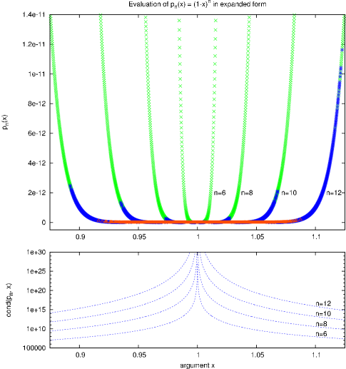
Figure 1: We report the evaluation of polynomials $p_{n}$ near the multiple root $x=1$ with the compensated Horner algorithm (CompHornerIsFaithul) and for multiplicity $n=6,8,10,12$. Each evaluation proved to be faithfully rounded thanks to the dynamic test is reported with a green cross. The faithful evaluations that are not detected to be so with the dynamic test are represented in blue. Finally, the evaluations that are not faithfully rounded are reported in red. The lower frame represents the condition number with respect to the argument $x$.

In the first experiment set, we evaluate the expanded form of polynomials $p_{n}(x)=(1-x)^{n}$, for degree $n=6,8,10,12$, at $2048$ equally spaced floating point entries being near the multiple root $x=1$. These evaluations are extremely ill-conditioned since

$$\operatorname{cond}(p_{n},x)=\left|\frac{1+|x|}{1-x}\right|^{n}.$$

These condition numbers are plotted in the lower frame of Figure 1 while $x$ varies around the root. These huge values have a sense since polynomials $p$ are exact in IEEE-754 double precision. Results are reported on Figure 1. The well known relation between the lost of accuracy and the nearness and the multiplicity of the root, i.e., the increasing of the condition number, is clearly illustrated. These results also illustrate that the dynamic bound becomes more pessimistic as the condition number increases. In next figures the horizontal axis does not represent the $x$ entry range anymore but the condition number which governs the whole behavior.

Figure 2: We report the relative accuracy of every polynomial evaluation ($y$ axis) with respect to the condition number ($x$ axis). Evaluation is performed with CompHornerIsFaithul (Algorithm LABEL:algo:FaithfulRoundingCompHorner). The color code is the same as for Figure 1. Leftmost vertical line is the a priori  sufficient condition (16) while the right one marks the inverse of the working precision ${\mathbf{u}}$. Broken line is the a priori  accuracy bound (15).

For the next experiment set, we first designed a generator of arbitrary ill-conditioned polynomial evaluations. It relies on the condition number definition (6). Given a degree $n$, a floating point argument $x$ and a targeted condition number $C$, it generates a polynomial $p$ with floating point coefficients such that $\operatorname{cond}(p,x)$ has the same order of magnitude as $C$. The principle of the generator is the following.

1. $\lfloor n/2\rfloor$ coefficients are randomly selected and generated such that $\,\widetilde{p}(x)=\sum|a_{i}||x|^{i}\approx C$,

2. the remaining coefficients are generated ensuring $|p(x)|\approx 1$ thanks to high accuracy computation.

Therefore we obtain polynomials $p$ such that $\operatorname{cond}(p,x)=\,\widetilde{p}(x)/|p(x)|\approx C$, for arbitrary values of $C$.

In this test set we consider generated polynomials of degree $50$ whose condition numbers vary from about $10^{2}$ to $10^{35}$. These huge condition numbers again have a sense here since the coefficients and the argument of every polynomial are floating point numbers. The results of the tests performed with CompHornerIsFaithul (Algorithm LABEL:algo:FaithfulRoundingCompHorner) are reported on Figure 2. As expected every polynomial with a condition number smaller than the a priori  bound (16) is faithfully evaluated with Algorithm LABEL:algo:FaithfulRoundingCompHorner —green plots at the left of the leftmost vertical line.

On Figure 2 we also see that evaluations with faithful rounding appear for condition numbers larger than the a priori  bound (16) — green and blue plots at the right of the leftmost vertical line. As expected a large part of these cases are detected by the dynamic test introduced in Theorem 9 —the green ones. Next experiment set comes back to this point. We also notice that the compensated Horner algorithm produces accurate evaluations for condition numbers up to about $1/{\mathbf{u}}$ —green and blue plots.

5.1.2 Significance of the dynamic error bound

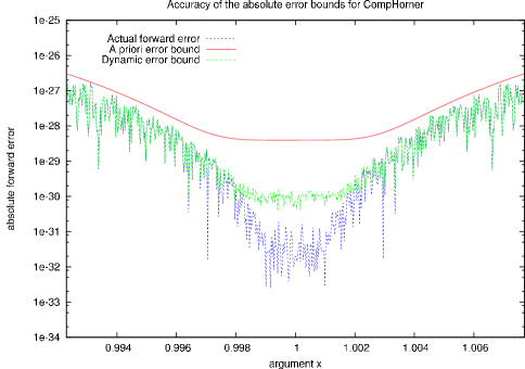
Figure 3: The dynamic error bound (20) compared to the a priori  bound (13) and to the actual forward error ($p(x)=(1-x)^{5}$ for $400$ entries on the $x$ axis).

We illustrate the significance of the dynamic error bound (20), compared to the a priori  error bound (13) and to the actual forward error. We evaluate the expanded form of $p(x)=(1-x)^{5}$ for $400$ points near $x=1$. For each value of the argument $x$, we compute $\mbox{{\sf CompHorner}}\left(p,x\right)$ (Algorithm LABEL:algo:CompHorner), the associated dynamic error bound (20) and the actual forward error. The results are reported on Figure 3.

As already noticed, the closer the argument is to the root $1$ (i.e., , the more the condition number increases), the more pessimistic becomes the a priori  error bound. Nevertheless our dynamic error bound is more significant than the a priori  error bound as it takes into account the rounding errors that occur during the computation.

5.2 Time performances

Table 2: Measured time performances for CompHorner, CompHornerIsFaithul and DDHorner. GCC denotes the GNU Compiler Collection and ICC denotes the Intel C/C++ Compiler.

		$\frac{{\sf CompHorner}}{{\sf Horner}}$	$\frac{{\sf CompHornerIsFaith}}{{\sf Horner}}$	$\frac{{\sf DDHorner}}{{\sf Horner}}$
Pentium 4, 3.00 GHz	GCC 3.3.5	3.77	5.52	10.00
	ICC 9.1	3.06	5.31	8.88
Athlon 64, 2.00 GHz	GCC 4.0.1	3.89	4.43	10.48
Itanium 2, 1.4 GHz	GCC 3.4.6	3.64	4.59	5.50
	ICC 9.1	1.87	2.30	8.78
		$\sim 2-4$	$\sim 4-6$	$\sim 5-10$

All experiments are performed using IEEE-754 double precision. Since the double-doubles [3, 7] are usually considered as the most efficient portable library to double the IEEE-754 double precision, we consider it as a reference in the following comparisons. For our purpose, it suffices to know that a double-double number $a$ is the pair $(a_{h},a_{l})$ of IEEE-754 floating point numbers with $a=a_{h}+a_{l}$ and $|a_{l}|\leq{\mathbf{u}}|a_{h}|$. This property implies a renormalisation step after every arithmetic operation with double-double values. We denote by DDHorner our implementation of the Horner algorithm with the double-double format, derived from the implementation proposed in [7].

We implement the three algorithms CompHorner, CompHornerIsFaith and DDHorner in a C code to measure their overhead compared to the Horner algorithm. We program these tests straightforwardly with no other optimization than the ones performed by the compiler. All timings are done with the cache warmed to minimize the memory traffic over-cost.

We test the running times of these algorithms for different architectures with different compilers as described in Table 2. Our measures are performed with polynomials whose degree vary from 5 to 200 by step of 5. For each algorithm, we measure the ratio of its computing time over the computing time of the classic Horner algorithm; we display the average time ratio over all test cases in Table 2.

The results presented in Table 2 show that the slowdown factor introduced by CompHorner compared to the classic Horner roughly varies between 2 and 4. The same slowdown factor varies between 4 and 6 for CompHornerIsFaithul and between 5 and 10 for DDHorner. We can see that CompHornerIsFaithul runs a most 2 times slower than CompHorner: the over-cost due to the dynamic test for faithful rounding is therefore quite reasonable. Anyway CompHorner and CompHornerIsFaithul run both significantly faster than DDHorner.

Remark 3.

We provide time ratios for IA’64 architecture (Itanium 2). Tested algorithms take benefit from IA’64 instructions, e.g., fma, but are not described in this paper.

6 Conclusion

Compensated Horner algorithm yields more accurate polynomial evaluation than the classic Horner iteration. Its accuracy behavior is similar to an Horner iteration performed in a doubled working precision. Hence compensated Horner may perform a faithful polynomial evaluation with IEEE-754 floating point arithmetic in the “round to the nearest” rounding mode. An a priori  sufficient condition with respect on the condition number that ensures such faithfulness has been defined thanks to the error free transformations.

These error free transformations also allow us to derive a dynamic sufficient condition that is more significant to check for faithful rounding with compensated Horner algorithm.

It is interesting to remark here that the significance of this dynamic bound can be improved easily —how to transform blue plots in green ones? Whereas bounding the error in the computation of the (polynomial) correcting term in Relation (18), a good approximate of the actual error could be computed (applying again CompHorner to the correcting term). Of course such extra computation will introduce more running time overhead not necessary useful —green plots are here! So it suffices to run such extra (but costly) checking only if the previous dynamic one fails (a similar strategy as in dynamic filters for geometric algorithms).

Compared to the classic Horner algorithm, experimental results exhibit reasonable over-costs for accurate polynomial evaluation (between 2 and 4) and even for this computation with a dynamic checking for faithfulness (between 4 and 6). Let us finally remark than such computation that provides as accuracy as if the working precision is doubled and a faithfulness checking is no more costly in term of running time than the “double-double” counterpart without any check.

Future work will be to consider subnormals results and also an adaptative algorithm that ensure faithful rounding for polynomials with an arbitrary condition number.

7 Appendix

Accuracy tests use next Matlab codes for algorithms Algorithm LABEL:algo:CompHorner (CompHorner) and Algorithm LABEL:algo:FaithfulRoundingCompHorner (CompHornerIsFaithul). Following Matlab convention, $p$ is represented as a vector p such that $p(x)=\sum_{i=0}^{n}\mathtt{p}(n-i+1)x^{i}$. We also recall that Matlab eps denotes the machine epsilon, which is the spacing between $1$ and the next larger floating point number, hence ${\mathbf{u}}=\mathtt{eps}/2$.

Algorithm 8.

Algorithm 9.

References

- [1] T. J. Dekker. A floating-point technique for extending the available precision. Numer. Math., 18:224–242, 1971.
- [2] S. Graillat, P. Langlois, and N. Louvet. Compensated Horner scheme. Technical report, University of Perpignan, France, July 2005.
- [3] Y. Hida, X. S. Li, and D. H. Bailey. Algorithms for quad-double precision floating point arithmetic. In N. Burgess and L. Ciminiera, editors, Proceedings of the 15th Symposium on Computer Arithmetic, Vail, Colorado, pages 155–162, Los Alamitos, CA, USA, 2001. Institute of Electrical and Electronics Engineers.
- [4] N. J. Higham. Accuracy and Stability of Numerical Algorithms. Society for Industrial and Applied Mathematics, Philadelphia, PA, USA, second edition, 2002.
- [5] IEEE Standards Committee 754. IEEE Standard for binary floating-point arithmetic, ANSI/IEEE Standard 754-1985. Institute of Electrical and Electronics Engineers, Los Alamitos, CA, USA, 1985. Reprinted in SIGPLAN Notices, 22(2):9-25, 1987.
- [6] D. E. Knuth. The Art of Computer Programming: Seminumerical Algorithms, volume 2. Addison-Wesley, Reading, MA, USA, third edition, 1998.
- [7] X. S. Li, J. W. Demmel, D. H. Bailey, G. Henry, Y. Hida, J. Iskandar, W. Kahan, S. Y. Kang, A. Kapur, M. C. Martin, B. J. Thompson, T. Tung, and D. J. Yoo. Design, implementation and testing of extended and mixed precision BLAS. ACM Trans. Math. Software, 28(2):152–205, 2002.
- [8] T. Ogita, S. M. Rump, and S. Oishi. Accurate sum and dot product. SIAM J. Sci. Comput., 26(6):1955–1988, 2005.
- [9] D. M. Priest. Algorithms for arbitrary precision floating point arithmetic. In P. Kornerup and D. W. Matula, editors, Proceedings of the 10th IEEE Symposium on Computer Arithmetic (Arith-10),Grenoble, France, pages 132–144, Los Alamitos, CA, USA, 1991. Institute of Electrical and Electronics Engineers.
- [10] S. M. Rump, T. Ogita, and S. Oishi. Accurate summation. Technical report, Hamburg University of Technology, Germany, Nov. 2005.