*

Abstract

In this paper we propose a Multi-Objective Ant Colony Optimization (MOACO) algorithm called CHAC, which has been designed to solve the problem of finding the path on a map (corresponding to a simulated battlefield) that minimizes resources while maximizing safety. CHAC has been tested with two different state transition rules: an aggregative function that combines the heuristic and pheromone information of both objectives and a second one that is based on the dominance concept of multiobjective optimization problems. These rules have been evaluated in several different situations (maps with different degree of difficulty), and we have found that they yield better results than a greedy algorithm (taken as baseline) in addition to a military behaviour that is also better in the tactical sense. The aggregative function, in general, yields better results than the one based on dominance.

1 Introduction

Prior to any combat manoeuvre, the unit commander must plan the best path to get to an position that is advantageous over the enemy in the tactical sense. This decision is conditioned by two criteria, speed and safety, which he must evaluate. The choice of a safe path is made when the enemy forces situation is not known, so the unit must move through hidden zones in order to avoid detection, which may correspond to a very long, and thus slower, path. On the other hand, the choice of a fast path is made when the unit is going to attack the enemy or if there are few hidden (safe) zones in the terrain and going through it may produce a lot of casualties. In any case, the computation of the best itinerary for the unit to reach the objective point is a very important tactical decision. We will try to make this decision in the paper by solving the what we have called the military unit path finding problem.

The military unit path finding problem is similar to the common path finding problem with some additional features and restrictions. It intends to find the best path from an origin to a destination point in the battlefield but keeping a balance between route speed and safety. The unit has an energy (health) and a resource level which are consumed when the unit moves through the path depending on the kind of terrain and difference of height, so the problem objectives are adapted to minimize the consumption of resources (which usually means walking as short/fast as possible) and the consumption of energy. In addition, there might be some enemies in the map (battlefield) which could shoot their weapons against the unit.

To solve the problem an Ant Colony System (ACS) algorithm has been adapted. It is a type of ACO [1, 2], which offers more control over the exploration and exploitation parts of search. In addition, some features to deal with the two objectives of the problem have been added (in [3] it can be found a survey of MO algorithms), so it is a MOACO algorithm (paper [4] presents a review of some of them). This problem had been solved so far using classical techniques like branch and bound or dynamic programming, which do not usually scale well with size, but to the best of our knowledge find no one that treat the problem as a multiobjective and solve it with a MOACO.

The rest of the paper is organized as follows: next section is devoted to a presentation of the problem we want to solve, followed in section 3 by a presentation of the CHAC algorithm. Experiments and results are presented in section 4, and conclusions are drawn in section 5, along with the future lines of development of this work.

2 The Problem

Our objective in this paper is to give the unit commander, or to a simulated unit in a combat training simulator, a tactical decision capability so that it will be able to calculate the best path to its target point in the battlefield considering the same factors that a commander would. The battlefield has been modeled as a square cell grid, every cell corresponding to a 500x500 meter zone in the real world.

The speed in a path is associated with the unit resources consumption because we have assigned a penalization to every cell related to the ‘difficulty’ of going through it and we have called this penalization resource cost of the cell. So, going through cells with more resource cost is more difficult and so more slow. Due to this justification, we refers to fast paths or paths with small resource cost.

Thus, the problem unit has two properties, a number of energy (which represent global health of unit soldiers or status of the unit vehicles) points and a number of resource (which represent unit supplies such as fuel, food and even moral) points. Its objective is to get to a target point with the maximum level in both properties.

The unit energy level is decremented in every cell of the path (the company depletes its human resources or vehicles suffer damage), which have a penalization called no combat casualties, depending on its type. In addition there is an extra penalization due to the impact of an enemy weapon in the cell. This value is calculated as combination of three other, the probability of enemy shoots, the probability of impact in the unit, and the damage it would produce to the unit.

Moreover every cell has an assigned resources penalty depending on the type of terrain. There is an extra penalty when the unit goes from a cell to other with different height (if it goes down, the penalty is small than if it goes up).

Besides cost in energy, and cost in resources, cells have the following properties:

• Type: there are four kinds of cells: normal (flat terrain), forest, water and obstacle, three different types of terrain and obstacle which means a cell that the unit cannot going through. There are several subtypes: it can be an enemy unit position, problem unit position, or the target point; it can also be affected by enemy fire (with one hundred levels of impact) or be lethal for the problem unit.

• Height: an integer number (between -3 and 3) which represents a level of depth or height of a cell.

We have implemented an application in Delphi 7 for Windows XP in order to create the problem scenarios (battlefields) and also to visualize the solutions obtained by CHAC. This application is available under request. Figure 1 shows an example of battlefield. It includes all typical features: enemy unit, obstacles, forest and water filled terrain accidents.

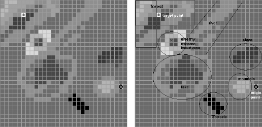
Figure 1: Map Example. It is a 30x30 map which shows some of the types and subtypes above mentioned. In left, and explanation of cells types is showed, because it is difficult to differ between different kinds of cells due to the black and white image. The example includes the problem unit (circle with black border), an enemy unit (square with gray border and mark with ’X’), the zone affected by enemy weapons (in different shades of light gray depending on the associated damage) surrounding the enemy and the objective point for the unit (circle with light gray border). The different shades in the same color models height (light color) and depth (dark color).

This implementation includes some constraints: problem and enemy units fill up exactly one cell (which corresponds with their size in real world). The problem unit as well as the target point must be located on the map; the presence of the enemy is optional. The unit can go only once through a cell and cannot go through cells occupied by an enemy or an obstacle, or cells with a cost in resources or energy bigger than what the unit has available. Some rules also apply to the line of sight, so that it behaves as realistically as possible.

3 The CHAC Algorithm

CHAC means Compañía de Hormigas Acorazadas or Armoured Ant Company; we have chosen this (admittedly a bit tongue-in-cheek) name to relate the ACO algorithms with the military scope of this application. It is an ACS adapted to deal with several objectives, that is, a MOACO or Multi-objective Ant Colony Optimization algorithm.

In order to approach it via an ACO algorithm, the problem must be transformed into a graph with weighted edges. Every cell in the map is considered a node in the graph with 8 edges connect it to every one of its neighbours (except in border cells). To deal with two objectives, there are two weights in every edge related to the cost of energy and resources, that is, a cost related to the energy expenses (cost assigned to the destination node of the edge) and other related to the consumption of resources if the unit moves from one cell to its neighbour following that edge (which depends on the types of both nodes and the height difference between them).

The algorithm implemented within CHAC is constructive which means that in every iteration, every ant builds a complete solution, if possible (there are some constraints, for example the unit cannot go through one node twice in the same path), by travelling through the graph. In order to guide this movement, the algorithm uses information of two kinds: pheromone and heuristic, that will be combined.

Since it is a multiobjective problem, CHAC uses two pheromone matrices, one per objective, and two heuristics functions (also matrices), following the BicriterionAnt algorithm designed by Iredi et al. in [5]. However, we decided to use an Ant Colony System (ACS) instead of an Ant System to have better control in the balance between exploration and exploitation by using the parameter q₀. We have implemented two state transition rules (which means two different algorithms), first one similar to the Iredi’s proposal and second one based on dominance of neighbours. The local and global updating formulas are based in the MACS-VRPTW algorithm proposed by Barán et al. in [6], with some changes due to the use of two pheromone matrices.

The objectives are named f, minimization the resources consumed in the path (speed maximization) and s, minimization the energy consumed in the path (safety).
The Heuristic Functions try to guide search between the start and the target point considering the most important factors for every objective. So, for edge (i,j) they are:

$$\eta_{f}(i,j)=\frac{\omega_{fr}}{Cr(i,j)}+\frac{\omega_{fd}}{Dist(j,T)}+\left(\omega_{fo}\cdot ZO(j)\right)$$ (1)

$$\eta_{s}(i,j)=\frac{\omega_{se}}{Ce(i,j)}+\frac{\omega_{sd}}{Dist(j,T)}+\left(\omega_{so}\cdot ZO(j)\right)$$ (2)

In Equation 1, Cr is the resource cost when moving from node i to node j, Dist is the Euclidean distance between two nodes (T is the target node of the problem) and ZO is a score (between 0 and 1) to a cell being 1 when the cell is hidden to all the enemies (or to all the cells in a radius when there are no enemies) and decreasing exponentially when it is seen. $\omega_{fr}$ , $\omega_{fd}$ and $\omega_{fo}$ are weights to assign relative importance to the terms in the formula. In this case, the most important term is the distance to target point because it searches for the fastest path. In second place is important the resources cost and only a little the hidden of the cell (it almost does not mind in a fast path).

In Equation 2, Ce is the energy cost of moving to node j, Dist and ZO is the same as the previous formula. $\omega_{se}$ , $\omega_{sd}$ and $\omega_{so}$ are again weights to assign relative importance to the terms in the formula, but in this case the most important are energy cost and hidden (both are to be considered in a safe path) and a little the distance to target point.

The Combined State Transition Rule (CSTR) is a formula used to decided which node j is the next in the construction of a solution (path) when the ant is at the node i, it is the pseudo-random-proportional rule used in ACS, but adapted to deal with a two objectives problem by combining the heuristic and pheromone information of both of them:

If (q $\leq$ q0)

$$j=\arg\max_{j\in N_{i}}\,\left\{\tau_{f}(i,j)^{\alpha\cdot\lambda}\cdot\tau_{s}(i,j)^{\alpha\cdot(1-\lambda)}\cdot\eta_{f}(i,j)^{\beta\cdot\lambda}\cdot\eta_{s}(i,j)^{\beta\cdot(1-\lambda)}\right\}$$ (3)

Else

$$P(i,j)=\left\{\begin{array}[]{ll}\frac{\displaystyle\tau_{f}(i,j)^{\alpha\cdot\lambda}\cdot\tau_{s}(i,j)^{\alpha\cdot(1-\lambda)}\cdot\eta_{f}(i,j)^{\beta\cdot\lambda}\cdot\eta_{s}(i,j)^{\beta\cdot(1-\lambda)}}{\displaystyle\sum\limits_{u\in N_{i}}\tau_{f}(i,u)^{\alpha\cdot\lambda}\cdot\tau_{s}(i,u)^{\alpha\cdot(1-\lambda)}\cdot\eta_{f}(i,u)^{\beta\cdot\lambda}\cdot\eta_{s}(i,u)^{\beta\cdot(1-\lambda)}}&\quad if\,j\in N_{i}\\ \\ \\ 0&\quad otherwise\\ \end{array}\right.$$ (4)

Where q₀ $\in$ [0,1] is the standard ACS parameter, q is a random value in [0,1]. $\tau_{f}$ and $\tau_{s}$ are the pheromone matrices and $\eta_{f}$ and $\eta_{s}$ are the heuristic functions for the objectives (Equations 1 and 2). All these matrices have a value for every edge (i,j). $\alpha$ and $\beta$ are the usual weighting parameters and N_i is the current feasible neighbourhood for the node i.
$\lambda$ $\in$ (0,1) is a user-defined parameter which sets the importance of the objectives in the search (this is an application created for a military user who decides which objective has more priority), so for instance, if the user decides to search for the fastest path, $\lambda$ will take a value close to 1 if he wants the safest path, it has to be close to 0. This value is kept during all the algorithm and for all the ants, unlike other bi-criterion implementations in which the parameter takes value 0 for first ant and it was growing for every ant until it takes a value 1 for the last one.

When an ant is building a solution path and it is placed at one node i, if q $\leq$ q₀ the best neighbour j is selected as the next (Equation 3). Otherwise, the algorithm decides which node is the next by using a roulette considering P(i,j) as probability for every feasible neighbour j (Equation 4).

The Dominance State Transition Rule (DSTR) is based on the dominance concept (see reference [3]), which is defined as follows (a dominates b):

$$a\succ b\;\;if:\quad\forall i\in 1,2,...,k\quad|\quad C_{i}(a)\leq C_{i}(b)\quad\wedge\quad\exists j\in 1,2,...k|C_{j}(a)<C_{j}(b)$$ (5)

Where a and b are two different vectors of k values (one per objective) and C is a cost function for every component in the vector. If it intends to minimize the cost and Equation 5 is true, then b is dominated by a.

So, in our problem there are two cost functions to evaluate the dominance between nodes. Actually these functions consider edges because they have assigned pheromone and heuristic information and combine them:

$$C_{f}(i,j)=\tau_{f}(i,j)^{\alpha\cdot\lambda}\cdot\eta_{f}(i,j)^{\beta\cdot\lambda}$$ (6)

$$C_{s}(i,j)=\tau_{s}(i,j)^{\alpha\cdot(1-\lambda)}\cdot\eta_{s}(i,j)^{\beta\cdot(1-\lambda)}$$ (7)

In addition there is a function which uses Equations 6 and 7:

$$D(i,j,u)=\left\{\begin{array}[]{ll}1&\quad if\>(i,j)\succ(i,u)\\ \\ 0&\quad otherwise\end{array}\right.$$ (8)

At last, the dominance state transition rule is as follows:

If (q $\leq$ q0)

$$j=\arg\max_{j\in N_{i}}\,\left\{\sum\limits_{u\in N_{i}}D(i,j,u)\quad\forall j\neq u\right\}$$ (9)

Else

$$P(i,j)=\left\{\begin{array}[]{ll}\frac{\displaystyle\left(\sum\limits_{u\in N_{i}}D(i,j,u)\right)+1}{\displaystyle\sum\limits_{k\in N_{i}}\left(\left(\sum\limits_{u\in N_{i}}D(i,k,u)\right)+1\right)}&\quad if\,j\in N_{i}\land j\neq u\land k\neq u\\ \\ \\ 0&\quad otherwise\\ \end{array}\right.$$ (10)

where all the parameters are the same as in Equations 3 and 4. This rule chooses the next node j in the path (when an ant is placed at node i) considering the number of neighbours dominated for every one. So if q $\leq$ q₀, the node which dominates more of the other neighbours is chosen, otherwise the probability roulette wheel is used. In Equation 10 we add 1 to avoid a 0 probability if no one dominates other neighbour.

There are two Evaluation Functions (one per objective, again):

$$F_{f}(Psol)=\sum\limits_{n\in Psol}[Cr(n-1,n)+\omega_{Ffo}\cdot(1-ZO(n))]$$ (11)

$$F_{s}(Psol)=\sum\limits_{n\in Psol}[Ce(n-1,n)+\omega_{Fso}\cdot(1-ZO(n))]$$ (12)

Where Psol is the solution path to evaluate and $\omega_{Ffo}$ and $\omega_{Fso}$ are weights related to the importance of visibility of the cells in the path. In Equation 11 its importance will be small, it is less important to hide in a fast path and it will be high in Equation 12 for the opposite reason. The other terms are the same that in Equations 1 and 2.

Since CHAC is an ACS, there are two levels of pheromone updating, local and global, which update two matrices at each level. The equations for Local Pheromone Updating (performed when a new node j is added to the path an ant is building) are:

$$\tau_{f}(i,j)=(1-\rho)\cdot\tau_{f}(i,j)+\rho\cdot\tau_{0f}$$ (13)

$$\tau_{s}(i,j)=(1-\rho)\cdot\tau_{s}(i,j)+\rho\cdot\tau_{0s}$$ (14)

Where $\rho$ in [0,1] is the common evaporation factor and $\tau_{0f}$, $\tau_{0s}$ are the initial amount of pheromone in every edge for every objective, respectively:

$$\tau_{0f}=\frac{1}{(numc\cdot MAX_{R})}$$ (15)

$$\tau_{0s}=\frac{1}{(numc\cdot MAX_{E})}$$ (16)

With numc as the number of cells in the map to solve, MAX_R is the maximum amount of resources going through a cell may require, and MAX_E is the maximum energy cost going through a cell may produce (in the worst case).

The equations for Global Pheromone Updating are:

$$\tau_{f}(i,j)=(1-\rho)\cdot\tau_{f}(i,j)+\rho/F_{f}$$ (17)

$$\tau_{s}(i,j)=(1-\rho)\cdot\tau_{s}(i,j)+\rho/F_{s}$$ (18)

Only the solutions inside the Pareto set will make the global pheromone updating once all the ants have finished of building paths in every iteration.

The pseudocode for CHAC is as follows:

Initialization of pheromone matrices with T0f and T0s

For i=1 to NUM_iterations

   For a=1 to NUM_ants

      ps=build_path(a)   /* Equations 1,2, [(3,4) or (6,7,8,9,10)] , 13,14 */

      evaluate(ps)   /* Equations 11,12 */

      if ps is non-dominated
         insert ps in Pareto_Set
         remove from Pareto_Set dominated solutions
      endif

   EndFor

   global_pheromone_updating   /* Equation 17,18 */

EndFor

4 Experiments and Results

We would like to first emphasize that the values for the parameters and weights affect the results because parameters guide the search and balance the exploration and exploitation of the algorithm, and weights set the importance of every term in the heuristics and evaluation function. We fine-tuned both in order to obtain a good behaviour in almost all the maps; the values found were $\alpha$ = 1, $\beta$ = 2, $\rho$ = 0.1 and q₀ = 0.4, in the three experiments we show in this section. The last value establishes a balance between exploration and exploitation, tending to exploration (but without abandoning exploitation altogether). The weights described in Equations 1, 2, 11 and 12 are set to give more importance to minimizing distance to target point and consumption of resources in the speed objective, and to give more importance to minimizing visibility and consumption of energy in the safety objective.

The user can only decide the value for $\lambda$ parameter, which gives relative importance to one objective over the other, so if it is near 1, finding fastest path would be more important and if it is near 0, the other way round.

As every MO algorithm, CHAC yields a set of non-dominated solutions from which the user chooses using his own criteria, since, usually he only wants one solution. But in this algorithm the resulting Pareto set is small (about five to ten different solutions on average, depending on the map size) because it only searches in the region of the ideal Pareto front delimited by the $\lambda$ parameter. We are going to represent in the results only ‘the best’ solution inside all the Pareto sets of 30 executions, considering better the solution with the smallest cost in the most significant criteria (depending on $\lambda$ value). In order to clarify this concept, there is not a best path, but paths enough good from the military point of view. These paths have been selected by the military participation of the project taking into account tactical considerations and the features of every battlefield.

CHAC have been implemented using the two state transition rules as two different algorithms. We are going to compare the results between both CHAC implementations (with the same parameter values), and both of them with a greedy approach which uses the same heuristic functions as cost functions (the pheromones has no equivalent in this algorithm), but using a dominance criterion to select the next node of the actual cell neighbourhood (it selects as next the node which dominates most of the others neighbours considering their cost in both objectives). This algorithm is quite simple, and sometimes does not even reach a solution because it gets into a loop situation (back and forth between a set of cells consuming all the resources or energy).

We have performed experiments on three different maps; two of them have cells of a single type of terrain (with different heights) in order to avoid problems of visualization due to the black and white figures. We executed every CHAC implementation 30 times with each extreme value for $\lambda$ parameter (0.9 and 0.1) in order to search for the fastest and the safest path (they cannot be 1 and 0 because always the two objectives must be considered). In every execution we chose the best solution (enough good from a military point of view) considering the objective we are minimizing and we make mean and standard deviation of them.

4.1 River and Forest Map

The first scenario is a 15x15 map with a river flowing between the start and the target point and a patch of forest. There is no enemy. The best of fast paths found and the best of safe paths found are shown in Figure 2, marked by circles.

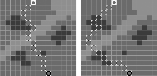
Figure 2: River and Forest map (forest cells in dark gray and water cells in light gray). Fastest (left) and safest (right) paths found. Both use forest cells to avoid being seen, but the latter goes through them to optimize safety.

	Combined State Transition Rule				Dominance State Transition Rule				Greedy
	Fastest ($\lambda$ = 0.9)		Safest ($\lambda$ = 0.1)		Fastest ($\lambda$ = 0.9)		Safest ($\lambda$ = 0.1)
	$F_{f}$	$F_{s}$	$F_{f}$	$F_{s}$	$F_{f}$	$F_{s}$	$F_{f}$	$F_{s}$
Best	22.198	85.768	25.704	61.189	22.214	80.075	27.274	61.833	NO SOLUTION
Mean	22.207	85.941	28.505	67.296	22.595	88.405	28.724	66.365
	$\pm$0.022	$\pm$0.436	$\pm$1.993	$\pm$3.360	$\pm$0.555	$\pm$3.127	$\pm$2.637	$\pm$2.881

Table 1: Results for River and Forest map. (500 iterations, 20 ants)

As it can be seen in Table 1, the cost of the solutions for the fastest path have a small standard deviation which means possibly CHAC has reach a quasi-optimal solution (small search space and enough iterations and ants to solve it). Mean and standard deviation in the objective which is not being minimized are logically worse, because it has little importance. DSTR implementation yields similar results even improving sometimes mean and standard deviation values in main objectives so, its solutions are more similar between executions (the algorithm has robustness).

Figure 2 (left) shows the fastest path found, which goes zigzagging, because the algorithm usually moves to the most hidden cells when there are no enemies (in a radius that can be set up by the user and which is 10 in this experiment), even in the search for the fastest path, but with less relevance. Forest cells obstruct the line of sight so the unit tends to move near them while goes rather directly to the target point. Figure 2 (right) shows the safest path found which moves in a less straightforward way and hides by moving near, and even inside forest cells (hidden is very important in safe paths) although it mean bigger resource cost (forest cells have more resource cost assigned than flat terrain).

4.2 Flat Terrain with Walls Map

The second map contains 30x30 cells, and represents a flat terrain with some ‘walls’, there is one enemy unit protecting the target cell (there are some cells affected by its weapons fire). The best of fast paths found and the best of safe paths found are shown in Figure 3. Cells with light gray border in the path are hidden to enemy.

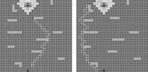
Figure 3: Flat Terrain with Walls, and one enemy shooting in a zone near the target point (the enemy is marked with ’X’, the cells surrounding it in light shades of gray are the zone of weapons impact and the other cells in light gray are the walls). Fastest (left) and safest (right) paths found by CHAC.

	Combined State Transition Rule				Dominance State Transition Rule				Greedy
	Fastest ($\lambda$ = 0.9)		Safest ($\lambda$ = 0.1)		Fastest ($\lambda$ = 0.9)		Safest ($\lambda$ = 0.1)
	$F_{f}$	$F_{s}$	$F_{f}$	$F_{s}$	$F_{f}$	$F_{s}$	$F_{f}$	$F_{s}$	$F_{f}$	$F_{s}$
Best	36.500	133.000	38.000	112.700	39.000	133.100	48.500	113.400	46.7	322.9
Mean	37.220	141.973	45.650	121.210	43.350	240.660	59.530	123.980
	$\pm$1.216	$\pm$2.904	$\pm$3.681	$\pm$10.425	$\pm$1.592	$\pm$85.254	$\pm$10.174	$\pm$8.119

Table 2: Results for the Flat Terrain with Walls map. (1000 iterations, 30 ants)

As it can be seen in Table 2, CHAC (in the two implementations) outperforms the greedy algorithm by almost 25% in resource cost and 75% in safety costs. The reason for this is that the greedy path is rather straight, which means low resource expenses; but, at the same time, it means the enemy sees the unit all the time (it moves through uncovered cells) and the safety cost is dramatically increased (it depends too much on cell visibility). The cost for fast path, which also depends on visibility, is increased too. The standard deviation is small in CSTR, but it grows a little in values of safest paths which could mean a bigger exploitation factor is needed. Again, in the DSTR implementation, results are similar to those obtained with CSTR, but with better standard deviation; however, its performance is poorer (even quite bad in one case) for the objectives it is not minimizing, which supports the theory that a higher exploitation level is needed in this scenario.

In Figure 3 (left), we can see the fastest path found; the unit moves in a curve mode in order to hide from enemy behind the walls (it consider the hidden of cells from the enemy cell). It surrounds this terrain elevations because resource cost of going through them is big. On the other hand, in Figure 3 (right) we can see the safest path found which moves surrounding the left side walls but remaining during more cells hide for the enemy. In both cases, the unit moves inside the zone affected by weapons choosing the less damaging cells, even in the safe case it arrives by a flank of the enemy unit where they have less fire power and this inflict less damage. It represents a good behaviour, very tactical in the case of safest path because attack to an enemy by the flank is one principle of military tactics.

4.3 Valleys and Mountains Map

This 45x45 map represents some big terrain accidents, with clear zones representing peaks (the more higher the more clearer) and dark zones representing valleys or cliffs. There are two enemies located in both peaks and the target point is behind one of them. The best of fast paths found and the best of safe paths found are shown in Figure 4. Circle cells mark the paths, those with light gray border in the path are hidden to both enemies.

Figure 4: Valleys and Mountains, with 2 enemy units (marked with ’X’) on watch. Fastest (left) and safest (right) path found.

	Combined State Transition Rule				Dominance State Transition Rule				Greedy
	Fastest ($\lambda$ = 0.9)		Safest ($\lambda$ = 0.1)		Fastest ($\lambda$ = 0.9)		Safest ($\lambda$ = 0.1)
	$F_{f}$	$F_{s}$	$F_{f}$	$F_{s}$	$F_{f}$	$F_{s}$	$F_{f}$	$F_{s}$
Best	70.500	334.600	84.500	285.800	73.500	374.300	76.000	354.600	NO SOLUTION
Mean	75.133	357.800	105.517	311.390	77.950	397.280	88.780	371.890
	$\pm$2.206	$\pm$9.726	$\pm$17.138	$\pm$19.541	$\pm$1.724	$\pm$11.591	$\pm$13.865	$\pm$7.522

Table 3: Results for Valleys and Mountains map. (2000 iterations, 70 ants)

As Table 3 shows, both implementations yield a low standard deviation, which means the algorithm is robust with respecto to initialization. CSTR implementation results may be nearer an optimal path, but in the DSTR case, the solutions have big costs (compared with the others), which means it needs more iterations or a greater exploitation factor to improve them. As in previous experiments, mean and standard deviation in the objectives that the algorithm is not minimizing are worse, because they have little importance. In this case, the differences between the cost of an objective when search minimizing this objective and when search minimizing the other are bigger than in the previous maps because the search space is bigger too.

In Figure 4 (left) we can see the fastest path found, the unit goes in a rather straight way to the target point, but without considering the hidden of cells (from the position of both enemies) so the safety cost increases dramatically. On the other hand, in Figure 4 (right) we can see the safest path found which represents a curve (distance to target point has little importance) which increases speed cost, but the unit goes through many hidden cells. This behaviour is excellent from military tactical point of view.

5 Conclusions and Future Work

In this paper we have described a MOACO algorithm called CHAC which tries to find the fastest and safest path, whose relative importance is set by the user, for a simulated military unit. This algorithm can use different state transition rules, and, in this papeer, two of them have been presented and tested. The first one combines heuristic and pheromone information of two objectives (Combined State Transition Rule, CSTR) and the second one is based on dominance over neighbours (Dominance State Transition Rule, DSTR).

The algorithm using both state transition rules has been tested in several different scenarios yielding very good results in a subjective assessment by the military staff of the project (Mr. Millán and Torrecillas) and being perfectly compatible with military tactics. They even offer good solutions in complicated maps in less time than a human expert would need. Moreover it is possible to observe an inherent emergent behaviour studying the solutions because it tends to be similar to those a real commander would, in many cases, take. In addition CHAC (using any state transition rule of the ones tested so far) outperforms a greedy algorithm. In the comparison between them, CHAC with CSTR yields better results in the same conditions, but CHAC with DSTR is more robust, yielding solutions that perform similarly, independently of the random initial conditions. If we increase exploitation level or iterations of algorithm, DSTR approach offers similar results to CSTR.

As future work, we will compare CHAC with path finding algorithms better than the simple greedy we have used here. From the algorithmic point of view, we will try to approach more systematically parameter setting, and investigate its performance in dynamic environments where, for instance, the enemy can move and shoot on sight. We will also try to evaluate its performance in environments with a hard time constraint, that is, in environments where the algorithm cannot run for an unlimited amount of time, but a limited and small one, which is usually the case in real combat situations. From the implementation point of view, it would be interesting to implement it within a real combat training simulator, that includes realistic values for most variables in this algorithm, including fuel consumption and casualties caused by projectile impact.

We will also try to approach scenario design more systematically, trying to describe its difficulty by looking at different aspects. This will allow us to assess different aspects of the algorithm and relate them to scenario difficulty, finding out which parameter combination is better for each scenario.

References

- [1] M. Dorigo and G. Di Caro. The ant colony optimization meta-heuristic. In D. Corne, M. Dorigo, and F. Glover, editors, New Ideas in Optimization, pages 11–32. McGraw-Hill, 1999.
- [2] M. Dorigo and T. Stützle. The ant colony optimization metaheuristic: Algorithms, applications, and advances. In G.A. Kochenberger F. Glover, editor, Handbook of Metaheuristics, pages 251–285. Kluwer, 2002.
- [3] Carlos A. Coello Coello, David A. Van Veldhuizen, and Gary B. Lamont. Evolutionary Algorithms for Solving Multi-Objective Problems. Kluwer Academic Publishers, 2002.
- [4] C. García-Martínez, O. Cordón, and F.Herrera. An empirical analysis of multiple objective ant colony optimization algorithms for the bi-criteria TSP. In ANTS 2004. Fourth International Workshop on. Ant Colony Optimization and Swarm Intelligence, number 3172 in LNCS, pages 61–72. Springer, 2004.
- [5] Steffen Iredi, Daniel Merkle, and Martin Middendorf. Bi-criterion optimization with multi colony ant algorithms. In E. Zitzler, K. Deb, L. Thiele, C. A. Coello Coello, and D. Corne, editors, Proceedings of the First International Conference on Evolutionary Multi-Criterion Optimization (EMO 2001), volume 1993 of Lecture Notes in Computer Science, pages 359–372, Berlin, 2001. Springer-Verlag.
- [6] B. Barán and M. Schaerer. A multiobjective ant colony system for vehicle routing problem with time windows. In IASTED International Multi-Conference on Applied Informatics, number 21 in IASTED IMCAI, pages 97–102, 2003. http://www.scopus.com/scopus/inward/record.url?eid=2-s2.0-1442302509&pa%rtner=40&rel=R4.5.0.