Local approximate inference algorithms

Abstract

We present a new local approximation algorithm for computing Maximum a Posteriori (MAP) and log-partition function for arbitrary exponential family distribution represented by a finite-valued pair-wise Markov random field (MRF), say $G$. Our algorithm is based on decomposition of $G$ into appropriately chosen small components; then computing estimates locally in each of these components and then producing a good global solution. Our algorithm for log-partition function provides provable upper and lower bounds on the correct value for arbitrary graph $G$. For MAP, our algorithm provides approximation with quantifiable error for arbitrary $G$. Specifically, we show that if the underlying graph $G$ either excludes some finite-sized graph as its minor (e.g. Planar graph) or has low doubling dimension (e.g. any graph with geometry), then our algorithm will produce solution for both questions within arbitrary accuracy. The running time of the algorithm is $\Theta(n)$ ($n$ is the number of nodes in $G$), with constant dependent on accuracy and either doubling dimension, or maximum vertex degree and the size of the graph that is excluded as a minor (e.g. $3$ for all Planar graphs).

We present a message-passing implementation of our algorithm for MAP computation using self-avoiding walk of graph. In order to evaluate the computational cost of this implementation, we derive novel tight bounds on the size of self-avoiding walk tree for arbitrary graph, which may be of interest in its own right.

As a consequence of our algorithmic result, we show that the normalized log-partition function (also known as free-energy) for a class of regular MRFs (e.g. Ising model on 2-dimensional grid) will converge to a limit, that is computable to an arbitrary accuracy, as the size of the MRF goes to infinity. This method, like classical sub-additivity method, is likely to be widely applicable.

I Introduction

Markov Random Field (MRF) [1] based exponential family of distribution allows for representing distributions in an intuitive parametric form. Therefore, it has been successful in modeling many applications (see, [2] for details). The key operational questions of interest are related to statistical inference: computing most likely assignment of (partially) unknown variables given some observations and computation of probability of an assignment given the partial observations (equivalently, computing log-partition function). In this paper, we study the question of designing efficient local algorithms for solving these inference problems.

I-A Previous work

The question of finding MAP (or ground state) of a given MRF comes up in many important application areas such as coding theory, discrete optimization, image denoising. Similarly, log-partition function is used in counting combinatorial objects [3], loss-probability computation in computer networks, [4], etc. Both problems are NP-hard for exact and even (constant) approximate computation for arbitrary graph $G$. However, the above stated applications require solving these problems using very simple algorithms. A popular successful approach for designing efficient heuristics has been as follows. First, identify a wide class of graphs that have simple algorithms for computing MAP and log-partition function. Then, for any given graph, approximately compute solution either by using that simple algorithm as a heuristic or in a more sophisticated case, by possibly solving multiple sub-problems induced by sub-graphs with good graph structures and then combining the results from these sub-problems to obtain a global solution.

Such an approach has resulted in many interesting recent results starting the Belief Propagation (BP) algorithm designed for Tree graph [1]. Since there is a vast literature on this topic, we will recall only few results. In our opinion, two important algorithms proposed along these lines of thought are the generalized belief propagation (BP) [5] and the tree-reweighted algorithm (TRW) [6, 7, 8]. Key properties of interest for these iterative procedures are the correctness of their fixed points and convergence. Many results characterizing properties of the fixed points are known starting from [5]. Various sufficient conditions for their convergence are known starting [9]. However, simultaneous convergence and correctness of such algorithms are established for only specific problems, e.g. [10, 11, 12].

Finally, we discuss two relevant results. The first result is about properties of TRW. The TRW algorithm provides provable upper bound on log-partition function for arbitrary graph [8]. However, to the best of authors’ knowledge the error is not quantified. The TRW for MAP estimation has a strong connection to specific Linear Programming (LP) relaxation of the problem [7]. This was made precise in a sequence of work by Kolmogorov [13], Kolmogorov and Wainwright [12] for binary MRF. It is worth noting that LP relaxation can be poor even for simple problems.

The second is an approximation algorithm proposed by Globerson and Jaakkola [14] to compute log-partition function using Planar graph decomposition (PDC). PDC uses techniques of [8] in conjunction with known result about exact computation of partition function for binary MRF when $G$ is Planar and the exponential family has a specific form (binary pairwise and multiplicative potentials). Their algorithm provides provable upper bound for arbitrary graph. However, they do not quantify the error incurred. Further, their algorithm is limited to binary MRF.

I-B Contributions

We propose a novel local algorithm for approximate computation of MAP and log-partition function. For any $\varepsilon>0$, our algorithm can produce an $\varepsilon$-approximate solution for MAP and log-partition function for arbitrary MRF $G$ as long as $G$ has either of these two properties: (a) $G$ has low doubling dimension (see Theorems 2 and 5), or (b) $G$ excludes a finite-sized graph as a minor (see Theorems 3 and 6). For example, Planar graph excludes $K_{3,3},K_{5}$ as a minor and thus our algorithm provides approximation algorithms for Planar graphs.

The running time of the algorithm is $\Theta(n)$, with constant dependent on $\varepsilon$ and (a) doubling dimension for doubling dimension graph, or (b) maximum vertex degree and size of the graph that is excluded as minor for minor-excluded graphs. For example, for $2$-dimensional grid graph, which has doubling dimension $O(1)$, the algorithm takes $C(\varepsilon)n$ time, where $\log\log C(\varepsilon)=O(1/\varepsilon)$. On the other hand, for a planar graph with maximum vertex degree a constant, i.e. $O(1)$, the algorithm takes $C^{\prime}(\varepsilon)n$ time, with $\log\log C^{\prime}(\varepsilon)=O(1/\varepsilon)$.

In general, our algorithm works for any $G$ and we can quantify bound on the error incurred by our algorithm. It is worth noting that our algorithm provides a provable lower bound on log-partition function as well unlike many of the previous results.

Our algorithm is primarily based on the following idea: First, decompose $G$ into small-size connected components say $G_{1},\dots,G_{k}$ by removing few edges of $G$. Second, compute estimates (either MAP or log-partition) in each of the $G_{i}$ separately. Third, combine these estimates to produce a global estimate while taking care of the error induced by the removed edges. We show that the error in the estimate depends only on the edges removed. This error bound characterization is applicable for arbitrary graph.

For obtaining sharp error bounds, we need good graph decomposition schemes. Specifically, we use a new, simple and very intuitive randomized decomposition scheme for graphs with low doubling dimensions. For minor-excluded graphs, we use a simple scheme based on work by Klein, Plotkin and Rao [15] and Rao [16] that they had introduced to study the gap between max-flow and min-cut for multicommodity flows. In general, as long as $G$ allows for such good edge-set for decomposing $G$ into small components, our algorithm will provide a good estimate.

To compute estimates in individual components, we use dynamic programming. Since each component is small, it is not computationally burdensome. However, one may obtain further simpler heuristics by replacing dynamic programming by other method such as BP or TRW for computation in the components.

In order to implement dynamic programing using message-passing approach, we use construction based on self-avoiding walk tree. Self-avoiding walk trees have been of interest in statistical physics for various reasons (see book by Madras and Slade [17]). Recently, Weitz [18] obtained a surprising result that connected computation of marginal probability of a node in any binary MRF to that of marginal probability of a root node in an appropriate self-avoiding walk tree. We use a direct adaption of this result for computing MAP estimate to design message passing scheme for MAP computation. In order to evaluate computation cost, we needed tight bound on the size on self-avoiding walk tree of arbitrary graph $G$. We obtain a novel characterization of size of self-avoiding walk tree within a factor $8$ for arbitrary graph $G$. This result should be of interest in its own right.

Finally, as a (somewhat unexpected) consequence of these algorithmic results, we obtain a method to establish existence of asymptotic limits of free energy for a class of MRF. Specifically, we show that if the MRF is $d$-dimensional grid and all node, edge potential functions are identical then the free-energy (i.e. normalized log-partition function) converges to a limit as the size of the grid grows to infinity. In general, such approach is likely to extend for any regular enough MRF for proving existence of such limit: for example, the result will immediately extend to the case when the requirement of node, edge potential being exactly the same is replaced by the requirement of they being chosen from a common distribution in an i.i.d. fashion.

I-C Outline

The paper is organized as follows. Section II presents necessary background on graphs, Markov random fields, exponential family of distribution, MAP estimation and log-partition function computation.

Section III presents graph decomposition schemes. These decomposition schemes are used later by approximation algorithms. We present simple, intuitive and $O(n)$ running time decomposition schemes for graphs with low doubling dimension and graphs that exclude finite size graph as a minor. Both of these schemes are randomized. The first scheme is our original contribution. The second scheme was proposed by Klein, Plotkin and Rao [15] and Rao [16].

Section IV presents the approximation algorithm for computing log-partition function. We describe how it provides upper and lower bound on log-partition function for arbitrary graph. Then we specialize the result for two graphs of interest: low doubling dimension and minor excluded graphs.

Section V presents the approximation algorithm for MAP estimation. We describe how it provides approximate estimate for arbitrary graph with quantifiable approximation error. Then we specialize the result for two graphs of interest: low doubling dimension and minor excluded graphs.

Section VI describes message passing implementation of the MAP estimation algorithm for binary pair-wise MRF for arbitrary $G$. This can be used by our approximation algorithm to obtain message passing implementation. This algorithm builds upon work by Weitz [18]. We describe a novel tight bound on the size of self-avoiding walk tree for any $G$. This helps in evaluating the computation time. The message passing implementation has similar computation complexity as the centralized algorithm.

Section VII presents an experimental evaluation of our algorithm for popular synthetic model on a grid graph. We compare our algorithm with TRW and PDC algorithms and show that our algorithm is very competent. An important feature of our algorithm is scalability.

Section VIII presents the implication of our algorithmic result in establishing asymptotic limit of free energy for regular MRFs, such as an Ising model on $d$-dimensional grid.

I-D How to read this paper: a suggestion

A reader, interested in obtaining a quick understanding of the results, should skip everything in Section III other than the definition of $(\varepsilon,\Delta)$ decomposition, and skip the Section VI completely. Reading these two sections at the very end may be helpful to parse the results with ease for all the readers.

II Preliminaries

This section provides the background necessary for subsequent sections. We begin with an overview of some graph theoretic basics. We then describe formalism of Markov random field and exponential family of distribution. We formulate the problem of log-partition function computation and MAP estimation for Markov random field. We conclude by stating precise definitions of approximate MAP estimation and approximate log-partition function computation.

II-A Graphs

An undirected graph $G=(V,E)$ consists of a set of vertices $V=\{1,\dots,n\}$ that are connected by set of edges $E\subset V\times V$. We consider only simple graphs, that is multiple edges between a pair of nodes or self-loops are not allowed. Let $\Gamma(v)=\{u\in V:(u,v)\in E\}$ denote the set of all neighboring nodes of $v\in V$. The size of the set $\Gamma(v)$ is the degree of node $v$, denoted as $d_{v}$. Let $d^{*}=\max_{v\in V}d_{v}$ be the maximum vertex degree in $G$. A clique of the graph $G$ is a fully-connected subset $C$ of the vertex set (i.e. $(u,v)\in E$ for all $u,v\in C$). Nodes $u$ and $v$ are called connected if there exists a path in $G$ starting from $u$ and ending at $v$ or vice versa since $G$ is undirected. Each graph $G$ naturally decomposes into disjoint sets of vertices $V_{1},\dots,V_{k}$ where for $1\leq i\leq k$, any two nodes say $u,v\in V_{i}$ are connected. The sets $V_{1},\dots,V_{k}$ are called the connected components of $G$.

We introduce a popular notion of dimension for graph $G$ (see recent works [19] [20] [21] for relevant details). Define $\mathbf{d_{G}}:V\times V\to\mathbb{R}_{+}$ as

$$\mathbf{d_{G}}(i,j)=\mbox{\sf length of the shortest path between $i$ and $j$}.$$

If $i=j$ then $\mathbf{d_{G}}(i,j)=0$ and if $i,j$ are not connected, then define $\mathbf{d_{G}}(i,j)=\infty$. It is easy to check that thus defined $\mathbf{d_{G}}$ is a metric on vertex set $V$. Define ball of radius $r\in\mathbb{R}_{+}$ around $v\in V$ as $\mathbf{B}(v,r)=\{u\in V:\mathbf{d_{G}}(u,v)<r\}$. Define

$$\rho(v,r) = \inf\{K\in\mathbb{N}:\exists~{}u_{1},\dots,u_{K}\in V,$$

$$\qquad\qquad\mathbf{B}(v,r)\subset\cup_{i=1}^{K}\mathbf{B}(u_{i},r/2)\}.$$

Then, $\rho(G)=\sup_{v\in V,r\in\mathbb{R}_{+}}\rho(v,r)$ is called the doubling dimension of graph $G$. Intuitively, this definition captures the notion of dimension $d$ in the Euclidian space $\mathbb{R}^{d}$. It follows from definition that for any graph $G$, $\rho(G)=O(\log_{2}n)$. We note the following property whose proof is presented in Appendix A.

Lemma 1

For any $v\in V$ and $r\in\mathbb{N}$, $|\mathbf{B}(v,2^{r})|\leq 2^{r\rho(\mathcal{M})}.$

Next, we introduce a class of graphs known as minor-excluded graphs (see a series of publications by Roberston and Seymour under ”the graph minor theory” project [22]). A graph $H$ is called minor of $G$ if we can transform $G$ into $H$ through an arbitrary sequence of the following two operations: (a) removal of an edge; (b) merge two connected vertices $u,v$: that is, remove edge $(u,v)$ as well as vertices $u$ and $v$; add a new vertex and make all edges incident on this new vertex that were incident on $u$ or $v$. Now, if $H$ is not a minor of $G$ then we say that $G$ excludes $H$ as a minor.

The explanation of the following statement may help understand the definition better: any graph $H$ with $r$ nodes is a minor of $K_{r}$, where $K_{r}$ is a complete graph of $r$ nodes. This is true because one may obtain $H$ by removing edges from $K_{r}$ that are absent in $H$. More generally, if $G$ is a subgraph of $G^{\prime}$ and $G$ has $H$ as a minor, then $G^{\prime}$ has $H$ as its minor. Let $K_{r,r}$ denote a complete bipartite graph with $r$ nodes in each partition. Then $K_{r}$ is a minor of $K_{r,r}$. An important implication of this is as follows: to prove property P for graph $G$ that excludes $H$, of size $r$, as a minor, it is sufficient to prove that any graph that excludes $K_{r,r}$ as a minor has property P. This fact was cleverly used by Klein et. al. [15].

II-B Markov random field

A Markov Random Field (MRF) is defined on the basis of an undirected graph $G=(V,E)$ in the following manner. Let $V=\{1,\dots,n\}$ and $E\subset V\times V$. For each $v\in V$, let $X_{v}$ be random variable taking values in some finite valued space $\Sigma_{v}$. Without loss of generality, lets assume that $\Sigma_{v}=\Sigma$ for all $v\in V$. Let $\mathbf{X}=(X_{1},\dots,X_{n})$ be the collection of these random variables taking values in $\Sigma^{n}$. For any subset $A\subset V$, we let $\mathbf{X}_{A}$ denote $\{X_{v}|v\in A\}$. We call a subset $S\subset V$ a cut of $G$ if by its removal from $G$ the graph decomposes into two or more disconnected components. That is, $V\backslash S=A\cup B$ with $A\cap B=\emptyset$ and there for any $a\in A,b\in B$, $(a,b)\notin E$. The $\mathbf{X}$ is called a Markov random field, if for any cut $S\subset V$, $\mathbf{X}_{A}$ and $\mathbf{X}_{B}$ are conditionally independent given $\mathbf{X}_{S}$, where $V\backslash S=A\cup B$.

By the Hammersley-Clifford theorem, any Markov random field that is strictly positive (i.e. $\Pr(\mathbf{X}=\mathbf{x})>0$ for all $\mathbf{x}\in\Sigma^{n}$) can be defined in terms of a decomposition of the distribution over cliques of the graph. Specifically, we will restrict our attention to pair-wise Markov random fields (to be defined precisely soon) only in this paper. This does not incur loss of generality for the following reason. A distributional representation that decomposes in terms of distribution over cliques can be represented through a factor graph over discrete variables. Any factor graph over discrete variables can be tranformed into a pair-wise Markov random field (see, [7] for example) by introducing auxiliary variables. As reader shall notice, the techniques of this paper can be extended to Markov random fields with higher-order interaction that contains hyper-edges.

Now, we present the precise definition of pair-wise Markov random field. We will consider distributions in exponential form. For each vertex $v\in V$ and edge $(u,v)\in E$, the corresponding potential functions are $\phi_{v}:\Sigma\to\mathbb{R}_{+}$ and $\psi_{uv}:\Sigma^{2}\to\mathbb{R}_{+}$. Then, the distribution of $\mathbf{X}$ is given as follows: for $\mathbf{x}\in\Sigma^{n}$,

$$\Pr[\mathbf{X}=\mathbf{x}] \propto \exp\left(\sum_{v\in V}\phi_{v}(x_{v})+\sum_{(u,v)\in E}\psi_{uv}(x_{u},x_{v})\right).~{}~{}$$ (1)

We note that the assumption of $\phi_{v},\psi_{uv}$ being non-negative does not incur loss of generality for the following reasons: (a) the distribution remains the same if we consider potential functions $\phi_{v}+C,\psi_{uv}+C$, for all $v\in V,(u,v)\in E$ with constant $C$; and (b) by selecting large enough constant, the modified functions will become non-negative as they are defined over finite discrete domain.

II-C Log-partition function

The normalization constant in definition (1) of distribution is called the partition function, $Z$. Specifically,

$$Z=\sum_{\mathbf{x}\in\Sigma^{n}}\exp\left(\sum_{v\in V}\phi_{v}(x_{v})+\sum_{(u,v)\in E}\psi_{uv}(x_{u},x_{v})\right).$$

Clearly, the knowledge of $Z$ is necessary in order to evaluate probability distribution or to compute marginal probabilities, i.e. $\Pr(X_{v}=x_{v})$ for $v\in V$. In applications in computer science, $Z$ corresponds to the number of combinatorial objects, in statistical physics normalized logarithm of $Z$ provides free-energy and in reversible stochastic networks $Z$ provides loss probability for evaluating quality of service.

In this paper, we will be interested in obtaining estimate of $\log Z$. Specifically, we will call $\hat{Z}$ as an $\varepsilon$-approximation of $Z$ if

$$(1-\varepsilon)\log Z\leq\log\hat{Z}\leq(1+\varepsilon)\log Z.$$

II-D MAP assignment

The maximum a posteriori (MAP) assignment $\mathbf{x}^{*}$ is one with maximal probability, i.e.

$$\mathbf{x}^{*}\in\arg\max_{\mathbf{x}\in\Sigma^{n}}\Pr[\mathbf{X}=\mathbf{x}].$$

Computing MAP assignment is of interest in wide variety of applications. In combinatorial optimization problem, $\mathbf{x}^{*}$ corresponds to an optimizing solution, in the context of image processing it can be used as the basis for image segmentation techniques and in error-correcting codes it corresponds to decoding the received noisy code-word.

In our setup, MAP assignment $\mathbf{x}^{*}$ corresponds to

$$\mathbf{x}^{*}\in\arg\max_{\mathbf{x}\in\Sigma^{n}}\left(\sum_{v\in V}\phi_{v}(x_{v})+\sum_{(u,v)\in E}\psi_{uv}(x_{u},x_{v})\right).$$

Define, $\mathcal{H}(\mathbf{x})=(\sum_{v\in V}\phi_{v}(x_{v})+\sum_{(u,v)\in E}\psi_{uv}(x_{u},x_{v}))$. We will be interested in obtaining an $\varepsilon$ estimate, say $\widehat{\mathbf{x}}$, of $\mathbf{x}^{*}$ such that

$$(1-\varepsilon)\mathcal{H}(\mathbf{x}^{*})\leq\mathcal{H}(\widehat{\mathbf{x}})\leq\mathcal{H}(\mathbf{x}^{*}).$$

III Graph decomposition

In this section, we introduce notion of graph decomposition. We describe very simple algorithms for obtaining decomposition for graphs with low doubling dimension and minor-excluded graphs. In the later sections, we will show that such decomposable graphs are good structures in the sense that they allow for local algorithms for approximately computing log-partition function and MAP.

III-A $(\varepsilon,\Delta)$ decomposition

Given $\varepsilon,\Delta>0$, we define notion of $(\varepsilon,\Delta)$ decomposition for a graph $G=(V,E)$. This notion can be stated in terms of vertex-based decomposition or edge-based decomposition.

We call a random subset of vertices $\mathcal{B}\subset V$ as $(\varepsilon,\Delta)$ vertex-decomposition of $G$ if the following holds: (a) For any $v\in V$, $\Pr(v\in\mathcal{B})\leq\varepsilon$. (b) Let $S_{1},\dots,S_{K}$ be connected components of graph $G^{\prime}=(V^{\prime},E^{\prime})$ where $V^{\prime}=V\backslash\mathcal{B}$ and $E^{\prime}=\{(u,v)\in E:u,v\in V^{\prime}\}$. Then, $\max_{1\leq k\leq K}|S_{k}|\leq\Delta$ with probability $1$.

Similarly, a random subset of edges $\mathcal{B}\subset E$ is called an $(\varepsilon,\Delta)$ edge-decomposition of $G$ if the following holds: (a) For any $e\in E$, $\Pr(e\in\mathcal{B})\leq\varepsilon$. (b) Let $S_{1},\dots,S_{K}$ be connected components of graph $G^{\prime}=(V^{\prime},E^{\prime})$ where $V^{\prime}=V$ and $E^{\prime}=E\backslash\mathcal{B}$. Then, $\max_{1\leq k\leq K}|S_{k}|\leq\Delta$ with probability $1$.

III-B Low doubling-dimension graphs

This section presents $(\varepsilon,\Delta)$ decomposition algorithm for graphs with low doubling dimension for various choice of $\varepsilon$ and $\Delta$. Such a decomposition algorithm can be obtained through a probabilistically padded decomposition for such graphs [20]. However, we present our (different) algorithm due to its simplicity. Its worth noting that this simplicity of the algorithm requires proof technique different (and more complicated) than that known in the literature.

We will describe algorithm for node-based $(\varepsilon,\Delta)$ decomposition. This will immediately imply algorithm for edge-based decomposition for the following reason: given $G=(V,E)$ with doubling dimension $\rho(G)$, consider graph of its edges $\mathcal{G}=(E,\mathcal{E})$ where $(e,e^{\prime})\in\mathcal{E}$ if $e,e^{\prime}$ shared a vertex in $G$. It is easy to check that $\rho(\mathcal{G})\leq 2\rho(G)+1$. Therefore, running algorithm for node-based decomposition on $\mathcal{G}$ will provide an edge-based decomposition.

The node-based decomposition algorithm for $G$ will be described for the metric space on $V$ with respect to the shortest path metric $\mathbf{d_{G}}$ introduced earlier. Clearly, it is not possible to have $(\varepsilon,\Delta)$ decomposition for any $\varepsilon$ and $\Delta$ values. As will become clear later, it is important to have such decomposition for $\varepsilon$ and $\Delta$ being not too large (specifically, we would like $\Delta=O(\log n)$). Therefore, we describe algorithm for any $\varepsilon>0$ and an operational parameter $K$. We will show that the algorithm will produce $(\varepsilon,\Delta)$ node-decomposition where $\Delta$ will depend on $\varepsilon,K$ and $\rho$.

Given $\varepsilon$ and $K$, define random variable $\mathbf{Q}$ over $\{1,\dots,K\}$ as

$$\Pr[\mathbf{Q}=i]=\begin{cases}\varepsilon(1-\varepsilon)^{i-1}&\mbox{if $1\leq i<K$}\\ (1-\varepsilon)^{K-1}&\mbox{if $i=K$}\end{cases}.$$

Define, $P_{K}=(1-\varepsilon)^{K-1}$. The algorithm Db-dim($\varepsilon,K$) described next essentially does the following: initially, all vertices are colored white. Iteratively, choose a white vertex arbitrarily. Let $u_{t}$ be vertex chosen in iteration $t$. Draw an independent random number as per distribution of $\mathbf{Q}$, say $\mathbf{Q}_{t}$. Select all white vertices that are at distance $\mathbf{Q}_{t}$ from $u_{t}$ in $\mathcal{B}$ and color them blue; color all white vertices at distance $<\mathbf{Q}_{t}$ from $u_{t}$ (including itself) as red. Repeat this process till no more white vertices are left. Output $\mathcal{B}$ (i.e. blue nodes) as the decomposition. Now, precise description of the algorithm.

Db-dim($\varepsilon,K$)  

• Initially, set iteration number $t=0$, $\mathcal{W}_{0}=V$, $\mathcal{B}_{0}=\emptyset$ and $\mathcal{R}_{0}=\emptyset$.

• Repeat the following till $\mathcal{W}_{t}\neq\emptyset$:

  • Choose an element $u_{t}\in\mathcal{W}_{t}$ uniformly at random.

  • Draw a random number $Q_{t}$ independently according to the distribution of $\mathbf{Q}$.

  • Update

    • $\mathcal{B}_{t+1}\leftarrow\mathcal{B}_{t}\cup\{w|\mathbf{d_{G}}(u_{t},w)=Q_{t}~{}\mbox{ and }~{}w\in\mathcal{W}_{t}\}$,

    • $\mathcal{R}_{t+1}\leftarrow\mathcal{R}_{t}\cup\{w|\mathbf{d_{G}}(u_{t},w)<Q_{t}~{}\mbox{ and }~{}w\in\mathcal{W}_{t}\}$,

    • $\mathcal{W}_{t+1}\leftarrow\mathcal{W}_{t}\cap\left(\mathcal{B}_{t+1}\cup\mathcal{R}_{t+1}\right)^{c}$.

  • Increment $t\leftarrow t+1$.

• Output $\mathcal{B}_{t}$.

 

We state property of the algorithm Db-dim($\varepsilon,K$) as follows.

Lemma 2

Given $G$ with doubling dimension $\rho=\rho(G)$ and $\varepsilon\in(0,1)$, let $K(\varepsilon,\rho)=\frac{12\rho}{\varepsilon}\log\left(\frac{24\rho}{\varepsilon}\right).$ Then Db-dim($\varepsilon,K(\varepsilon,\rho)$) produces random output $\mathcal{B}\subset V$ that is $(2\varepsilon,\Delta(\varepsilon,\rho))$ node-decomposition of $G$ with $\Delta(\varepsilon,\rho)\leq K(\varepsilon,\rho)^{2\rho}$. The algorithm takes $O(C(\varepsilon,\rho)n)$ amount of time to produce $\mathcal{B}$, where $C(\varepsilon,\rho)=K(\varepsilon,\rho)^{2\rho}$.

Before presenting the proof of Lemma 2, we state the following important corollary for designing efficient algorithm.

Corollary 1

Let $\varepsilon\leq 1,\rho$ be such that $\rho\log(\rho/\varepsilon)=o(\log\log n)$. Then Db-dim($\varepsilon/2,K(\varepsilon/2,\rho)$) produces $(\varepsilon,\log^{1/L}n)$ node-decomposition for any finite (not scaling with $n$) $L$ .

Proof:

Since $\rho\log(\rho/\varepsilon)=o(\log\log n)$, we have that

$$2\rho\left(\log\frac{24\rho}{\varepsilon}+\log\log\frac{48\rho}{\varepsilon}\right)=o(\log\log n).$$

Therefore, by definition of $K(\varepsilon,\rho)$ we have that

$$K(\varepsilon/2,\rho)^{2\rho} = \exp\left(2\rho\left[\log\frac{24\rho}{\varepsilon}+\log\log\frac{48\rho}{\varepsilon}\right]\right)$$ (2)

$$= \exp\left(o(\log\log n)\right)$$

$$\leq \log^{1/L}n,$$

for any finite $L$. The last inequality follows from the definition of notation $o(\cdot)$. Now, Lemma 2 implies the desired claim. ∎

Proof:

(Lemma 2) To prove claim of Lemma, we need to show two properties of the output set $\mathcal{B}$ for given $\varepsilon$ and $K=K(\varepsilon,\rho)$: (a) for any $v\in V$, $\Pr(v\in\mathcal{B})\leq 2\varepsilon$; (b) the graph $G$, upon removal of $\mathcal{B}$, decomposes into connected component each of size at most $K^{2\rho}$.

Before, we prove (a) and (b), lets bound the running time of the algorithm. Note that the algorithm runs for at most $n$ iterations. In each iteration, the algorithm needs to check nodes that are within distance $K(\varepsilon,\rho)$ of the randomly chosen node. Therefore, total number of operations performed is at most $O(K(\varepsilon,\rho)^{2\rho})$. Thus, the total running time is $O(nK(\varepsilon,\rho)^{2\rho})$. Now we first justify (a) and then (b).

Proof of (a). To prove (a), we use the following Claim.

Claim 1

Consider metric space $\mathcal{M}=(V,\mathbf{d_{G}})$ with $|V|=n$. Let $\mathcal{B}\subset V$ be the random set that is output of decomposition algorithm with parameter $(\varepsilon,K)$ applied to $\mathcal{M}$. Then, for any $v\in V$

$$\Pr[v\in\mathcal{B}]\leq\varepsilon+P_{K}|\mathbf{B}(v,K)|,$$

where $\mathbf{B}(v,K)$ is the ball of radius $K$ in $\mathcal{M}$ with respect to the $\mathbf{d_{G}}$.

Proof:

(Claim 1) The proof is by induction on the number of points $n$ over which metric space is defined. When $n=1$, the algorithm chooses only point as $u_{0}$ in the initial iteration and hence it can not be part of the output set $\mathcal{B}$. That is, for this only point, say $v$,

$$\Pr[v\in\mathcal{B}]=0\leq\varepsilon+P_{K}|\mathbf{B}(v,K)|.$$

Thus, we have verified the base case for induction ($n=1$).

As induction hypothesis, suppose that the Claim 1 is true for any metric space on $n$ points with $n<N$ for some $N\geq 2$. As the induction step, we wish to establish that for a metric space $\mathcal{M}=(V,\mathbf{d_{G}})$ with $|V|=N$, the Claim 1 is true. For this, consider any point $v\in V$. Now consider the first iteration of the algorithm applied to $\mathcal{M}$. The algorithm picks $u_{0}\in V$ uniformly at random in the first iteration. Given $v$, depending on the choice of $u_{0}$ we consider four different cases (or events).

Case 1. This case corresponds to event $E_{1}$ where the chosen random $u_{0}$ is equal to point $v$ of our interest. By definition of algorithm, under the event $E_{1}$, $v$ will never be part of output set $\mathcal{B}$. That is,

$$\Pr[v\in\mathcal{B}|E_{1}]=0~{}\leq~{}\varepsilon+P_{K}|\mathbf{B}(v,K)|.$$

Case 2. Now, suppose $u_{0}$ be such that $v\neq u_{0}$ and $\mathbf{d_{G}}(u_{0},v)<K$. Call this event $E_{2}$. Further, depending on choice of random number $Q_{0}$, define events:

$$E_{21}=\{\mathbf{d_{G}}(u_{0},v)<Q_{0}\},~{}E_{22}=\{\mathbf{d_{G}}(u_{0},v)=Q_{0}\},~{}\mbox{and}~{}$$

$$~{}E_{23}=\{\mathbf{d_{G}}(u_{0},v)>Q_{0}\}.$$

By definition of algorithm, when $E_{21}$ happens, $v$ is selected as part of $\mathcal{R}_{1}$ and hence can never be part of output $\mathcal{B}$. When $E_{22}$ happens $v$ is selected as part of $\mathcal{B}_{1}$ and hence it is definitely part of output set $\mathcal{B}$. When $E_{23}$ happens, $v$ is neither selected in set $\mathcal{R}_{1}$ nor selected in set $\mathcal{B}_{1}$. It is left as an element of the set $\mathcal{W}_{1}$. This new set $\mathcal{W}_{1}$ has points $<N$. The original metric $\mathbf{d_{G}}$ is still a metric on points of $\mathcal{W}_{1}$. By definition, the algorithm only cares about $(\mathcal{W}_{1},\mathbf{d_{G}})$ in future and is not affected by its decisions in past. Therefore, we can invoke induction hypothesis which implies that if event $E_{23}$ happens then the probability of $v\in\mathcal{B}$ is bounded above by $\varepsilon+P_{K}|\mathbf{B}(v,K)|$. Finally, let us relate the $\Pr[E_{21}|E_{2}]$ with $\Pr[E_{22}|E_{2}]$. Suppose $\mathbf{d_{G}}(u_{0},v)=\ell<K$. By definition of probability distribution of $\mathbf{Q}$, we have

$$\Pr[E_{22}|E_{2}] = \varepsilon(1-\varepsilon)^{\ell-1}.$$ (3)

$$\Pr[E_{21}|E_{2}] = (1-\varepsilon)^{K-1}+\sum_{j=\ell+1}^{K-1}\varepsilon(1-\varepsilon)^{j-1}$$ (4)

$$= (1-\varepsilon)^{\ell}.$$

That is,

$$\Pr[E_{22}|E_{2}]=\frac{\varepsilon}{1-\varepsilon}\Pr[E_{21}|E_{2}].$$

Let $q\stackrel{{\scriptstyle\triangle}}{{=}}\Pr[E_{21}|E_{2}]$. Then,

$$\Pr[v\in\mathcal{B}|E_{2}] = \Pr[v\in\mathcal{B}|E_{21}\cap E_{2}]\Pr[E_{21}|E_{2}]$$ (5)

$$~{}~{}+\Pr[v\in\mathcal{B}|E_{22}\cap E_{2}]\Pr[E_{22}|E_{2}]$$

$$~{}~{}~{}+\Pr[v\in\mathcal{B}|E_{23}\cap E_{2}]\Pr[E_{23}|E_{2}]$$

$$= \frac{\varepsilon q}{1-\varepsilon}+(\varepsilon+P_{K}|\mathbf{B}(v,K)|)\left(1-\frac{q}{1-\varepsilon}\right)$$

$$= \varepsilon+P_{K}|\mathbf{B}(v,K)|-\frac{qP_{K}|\mathbf{B}(v,K)|}{1-\varepsilon}$$

$$\leq \varepsilon+P_{K}|\mathbf{B}(v,K)|.$$

Case 3. Now, suppose $u_{0}\neq v$ is such that $\mathbf{d_{G}}(u_{0},v)=K$. Call this event $E_{3}$. Further, let event $E_{31}=\{Q_{0}=K\}$. Due to independence of selection of $Q_{0}$, $\Pr[E_{31}|E_{3}]=P_{K}$. Under event $E_{31}\cap E_{3}$, $v\in\mathcal{B}$ with probability $1$. Therefore,

$$\Pr[v\in\mathcal{B}|E_{3}] = \Pr[v\in\mathcal{B}|E_{31}\cap E_{3}]\Pr[E_{31}|E_{3}]$$ (6)

$$+\Pr[v\in\mathcal{B}|E^{c}_{31}\cap E_{3}]\Pr[E^{c}_{31}|E_{3}]$$

$$= P_{K}+\Pr[v\in\mathcal{B}|E_{31}^{c}\cap E_{3}](1-P_{K}).~{}~{}$$

Under event, $E^{c}_{31}\cap E_{3}$, we have $v\in\mathcal{W}_{1}$ and the remaining metric space $(\mathcal{W}_{1},\mathbf{d_{G}})$. This metric space has $<N$ points. Further, the ball of radius $K$ around $v$ with respect to this new metric space has at most $|\mathbf{B}(v,K)|-1$ points (this ball is with respect to the original metric space $\mathcal{M}$ of $N$ points). We can invoke induction hypothesis for this new metric space (because of similar justification as in the previous case) to obtain

$$\Pr[v\in\mathcal{B}|E^{c}_{31}\cap E_{3}] \leq \varepsilon+P_{K}(|\mathbf{B}(v,K)|-1).$$ (7)

From (6) and (7), we have

$$\Pr[v\in\mathcal{B}|E_{3}] \leq P_{K}+(1-P_{K})(\varepsilon+P_{K}(|\mathbf{B}(v,K)|-1))$$ (8)

$$= \varepsilon(1-P_{K})+P_{K}|\mathbf{B}(v,K)|$$

$$~{}~{}+P_{K}^{2}(1-|\mathbf{B}(v,K)|)$$

$$\leq \varepsilon+P_{K}|\mathbf{B}(v,K)|.$$

Case 4. Finally, let $E_{4}$ be the event that $\mathbf{d_{G}}(u_{0},v)>K$. Then, at the end of the first iteration of the algorithm, we again have the remaining metric space $(\mathcal{W}_{1},\mathbf{d_{G}})$ such that $|\mathcal{W}_{1}|<N$. Hence, as before by induction hypothesis we will have

$$\Pr[v\in\mathcal{B}|E_{4}]\leq\varepsilon+P_{K}|\mathbf{B}(v,K)|.$$

Now, the four cases are exhaustive and disjoint. That is, $\cup_{i=1}^{4}E_{i}$ is the universe. Based on the above discussion, we obtain the following.

$$\Pr[v\in\mathcal{B}] = \sum_{i=1}^{4}\Pr[v\in\mathcal{B}|E_{i}]\Pr[E_{i}]$$ (9)

$$\leq \left(\max_{i=1}^{4}\Pr[v\in\mathcal{B}|E_{i}]\right)\left(\sum_{i=1}^{4}\Pr[E_{i}]\right)$$

$$\leq \varepsilon+P_{K}|\mathbf{B}(v,K)|.$$

This completes the proof of Claim 1. ∎

Now, we will use Claim 1 to complete the proof of (a). Lemma 1 for metric space with doubling dimension $\rho$ and integer distances imply that,

$$\left|\mathbf{B}(v,K)\right|\leq\left|\mathbf{B}\left(v,2^{\lceil\log_{2}K\rceil}\right)\right|\leq 2^{\rho(\log_{2}K+1)}=(2K)^{\rho}.$$

Therefore, it is sufficient to show that

$$P_{K}(2K)^{\rho}\leq\varepsilon.$$

Recall that $K(\varepsilon,\rho)=\frac{12\rho}{\varepsilon}\log\left(\frac{24\rho}{\varepsilon}\right),$ and $P_{K}=(1-\varepsilon)^{K-1}$. Hence,

$$K = \frac{12\rho}{\varepsilon}\log\left(\frac{24\rho}{\varepsilon}\right)$$ (10)

$$\geq \frac{6\rho}{\varepsilon}\left(\log\left(\frac{24\rho}{\varepsilon}\right)+\log\log\left(\frac{24\rho}{\varepsilon}\right)\right)$$

$$= \frac{6\rho}{\varepsilon}\log 2K.$$

Now since $K\geq 3$, we obtain that $K-1\geq\frac{4\rho}{\varepsilon}\log 2K$. Then, from $K\geq\frac{1}{\varepsilon}$ and $\rho\geq 1$,

$$K-1\geq\frac{2\rho}{\varepsilon}\log 2K+\frac{2}{\varepsilon}\log\frac{1}{\varepsilon}.$$

Note that $\log(1-\varepsilon)^{-1}\geq\log(1+\varepsilon)\geq\frac{\varepsilon}{2},~{}~{}\mbox{for}~{}\varepsilon\in(0,1).$ Hence,

$$(K-1)\log(1-\varepsilon)^{-1}\geq\rho\log 2K+\log\frac{1}{\varepsilon},$$

which implies

$$(1-\varepsilon)^{K-1}(2K)^{\rho}\leq\varepsilon.$$

This completes the proof of (a) of Lemma 2.

Proof of (b). First we give some notations. Define $R_{t}=\mathcal{R}_{t}-\mathcal{R}_{t-1}$, $B_{t}=\mathcal{B}_{t}-\mathcal{B}_{t-1}$ and

$$\partial R_{t}=\{v\in V:v\notin R_{t}\mbox{~{}and~{}}\exists~{}v^{\prime}\in R_{t}\mbox{~{}s.t.~{}}\mathbf{d_{G}}(v,v^{\prime})=1\}.$$

The followings are straightforward observations implied by the algorithm: for any $t\geq 0$, (i) $R_{t}\cap\mathcal{R}_{t-1}=\emptyset$, (ii) $B_{t}\cap\mathcal{B}_{t-1}=\emptyset$, (iii) $R_{t}\subset\mathbf{B}(u_{t-1},Q_{t-1})$, and (iv) $B_{t}\subset\mathbf{B}(u_{t-1},Q_{t-1}+1)-\mathbf{B}(u_{t-1},Q_{t-1})$. Now, we state a crucial claim for proving (b).

Claim 2

For all $t\geq 0$, $\partial R_{t}\subset\mathcal{B}_{t}$.

Proof:

(Claim 2) We prove it by induction. Initially, $\partial R_{0}=\mathcal{B}_{0}=\emptyset$ and hence the claim is trivial. At the end of the first iteration, by definition of the algorithm

$$R_{1}=\mathcal{R}_{1}=\mathbf{B}(u_{0},Q_{0}),~{}\mbox{and}~{}$$

$$B_{1}=\mathcal{B}_{1}=\mathbf{B}(u_{0},Q_{0}+1)-\mathbf{B}(u_{0},Q_{0}).$$

Therefore, by definition $\partial R_{1}=\mathcal{B}_{1}$. Thus, the base case of induction is verified. Now, as the hypothesis for induction suppose that $\partial R_{t}\subset\mathcal{B}_{t}$ for all $t\leq\ell$, for some $\ell\geq 1$. As induction step, we will establish that $\partial R_{\ell+1}\subset\mathcal{B}_{\ell+1}$.

Suppose to the contrary, that $\partial R_{\ell+1}\not\subset\mathcal{B}_{\ell+1}$. That is, there exists $v\in\partial R_{\ell+1}$ such that $v\not\in\mathcal{B}_{\ell}$. By definition of algorithm, we have

$$R_{\ell+1}=\mathbf{B}(u_{\ell},Q_{\ell})-(\mathcal{R}_{\ell}\cup\mathcal{B}_{\ell}).$$

Therefore,

$$\partial R_{\ell+1}\subset(\mathbf{B}(u_{\ell},Q_{\ell}+1)-\mathbf{B}(u_{\ell},Q_{\ell}))\cup\mathcal{R}_{\ell}\cup\mathcal{B}_{\ell}.$$

Again, by definition of the algorithm we have

$$B_{\ell+1}=\mathbf{B}(u_{\ell},Q_{\ell}+1)-\mathbf{B}(u_{\ell},Q_{\ell})-\mathcal{R}_{\ell}-\mathcal{B}_{\ell}.$$

Therefore, $v\in B_{\ell+1}$ or $v\in\mathcal{R}_{\ell}\cup\mathcal{B}_{\ell}$. Recall that by definition of algorithm $\mathcal{B}_{\ell}\cap\mathcal{R}_{\ell}=\emptyset$. Since we have assumed that $v\notin\mathcal{B}_{\ell+1}$, it must be that $v\in\mathcal{R}_{\ell}$. That is, there exists $\ell^{\prime}\leq\ell$ such that $v\in R_{\ell^{\prime}}$. Now since $v\in\partial R_{\ell+1}$ by assumption, it must be that there exists $v^{\prime}\in R_{\ell+1}$ such that $\mathbf{d_{G}}(v,v^{\prime})=1$. Since by definition $R_{\ell+1}\cap R_{\ell^{\prime}}=\emptyset$, we have $v^{\prime}\in\partial R_{\ell^{\prime}}$. By induction hypothesis, this implies that $v^{\prime}\in\mathcal{B}_{\ell^{\prime}}\subset\mathcal{B}_{\ell}$. That is, $\mathcal{B}_{\ell}\cap R_{\ell+1}\neq\emptyset$, which is a contradiction to the definition of our algorithm. That is, our assumption that $\partial R_{\ell+1}\not\subset\mathcal{B}_{\ell+1}$ is false. Thus, we have established the inductive step. This completes the induction argument and proof of the Claim 2. ∎

Now when the algorithm terminates (which must happen within $n$ iterations), say the output set is $\mathcal{B}_{T}$ and $V-\mathcal{B}_{T}=\mathcal{R}_{T}$ for some $T$. As noted above, $\mathcal{R}_{T}$ is a union of disjoint sets $R_{1},\dots,R_{T}$. We want to show that $R_{i},R_{j}$ are disconnected for any $1\leq i<j\leq T$ using Claim 2. Suppose to the contrary that they are connected. That is, there exists $v\in R_{i}$ and $v^{\prime}\in R_{j}$ such that $\mathbf{d_{G}}(v,v^{\prime})=1$. Since $R_{i}\cap R_{j}=\emptyset$, it must be that $v^{\prime}\in\partial R_{i},v\in\partial R_{j}$. From Claim 2 and fact that $\mathcal{B}_{t}\subset\mathcal{B}_{t+1}$ for all $t$, we have that $R_{i}\cap\mathcal{B}\neq\emptyset,R_{j}\cap\mathcal{B}\neq\emptyset$. This is contrary to the definition of the algorithm. Thus, we have established that $R_{1},\dots,R_{T}$ are disconnected components whose union is $V-\mathcal{B}_{T}$. By definition, each of $R_{i}\subset\mathbf{B}(u_{i-1},K)$. Thus, we have established that $V-\mathcal{B}_{T}$ is made of connected components, each of which is contained inside balls of radius $K$ with respect to $\mathbf{d_{G}}$. Since, $G$ has doubling dimension $\rho$, Lemma 1 implies that the size of any ball of radius $K$ is at most $(2K)^{\rho}$. Given choice of $\varepsilon\leq 1$ and $\rho\geq 1$, we have that $K\geq 2$. Therefore, $(2K)^{\rho}\leq K^{2\rho}$. This completes the proof of (b) and that of Lemma 2. ∎

III-C Minor-excluded graphs

Here we describe a simple and explicit construction of decomposition for graphs that exclude certain finite sized graphs as their minor. This scheme is a direct adapation of a scheme proposed by Klein, Plotkin, Rao [15] and Rao [16]. We describe an $(\varepsilon,\Delta)$ node-decomposition scheme. Later, we describe how it can be modified to obtain $(\varepsilon,\Delta)$ edge-decomposition.

Suppose, we are given graph $G$ that excludes graph $K_{r,r}$ as minor. Recall that if a graph excludes some graph $G_{r}$ of $r$ nodes as its minor then it excludes $K_{r,r}$ as its minor as well. In what follows and the rest of the paper, we will always assume $r$ to be some finite number that does not scale with $n$ (the number of nodes in $G$). The following algorithm for generating node-decomposition uses parameter ${\Lambda}$. Later we shall relate the parameter ${\Lambda}$ to the decomposition property of the output.

Minor-v($G,r,{\Lambda}$)   

• Input is graph $G=(V,E)$ and $r,{\Lambda}\in{\mathbb{N}}$. Initially, $i=0$, $G_{0}=G$, $\mathcal{B}=\emptyset$.

• For $i=0,\dots,r-1$, do the following.

  • Let $S^{i}_{1},\dots,S^{i}_{k_{i}}$ be the connected components of $G_{i}$.

  • For each $S^{i}_{j},1\leq j\leq k_{i}$, pick an arbitrary node $v_{j}\in S^{i}_{j}$.

    • Create a breadth-first search tree $\mathcal{T}^{i}_{j}$ rooted at $v_{j}$ in $S^{i}_{j}$.

    • Choose a number $L^{i}_{j}$ uniformly at random from $\{0,\dots,{\Lambda}-1\}$.

    • Let $\mathcal{B}^{i}_{j}$ be the set of nodes at level $L^{i}_{j},{\Lambda}+L^{i}_{j},2{\Lambda}+L^{i}_{j},\dots$ in $\mathcal{T}^{i}_{j}$.

    • Update $\mathcal{B}=\mathcal{B}\cup_{j=1}^{k_{i}}\mathcal{B}^{i}_{j}$.

  • set $i=i+1$.

• Output $\mathcal{B}$ and graph $G^{\prime}=(V,E\backslash\mathcal{B})$.

 

As stated above, the basic idea is to use the following step recursively (upto depth $r$ of recursion): in each connected component, say $S$, choose a node arbitrarily and create a breadth-first search tree, say $\mathcal{T}$. Choose a number, say $L$, uniformly at random from $\{0,\dots,{\Lambda}-1\}$. Remove (and add to $\mathcal{B}$) all nodes that are at level $L+k{\Lambda},k\geq 0$ in $\mathcal{T}$. Clearly, the total running time of such an algorithm is $O(r(n+|E|))$ for a graph $G=(V,E)$ with $|V|=n$; with possible parallel implementation across different connected components.

Figure 1 explains the algorithm for a line-graph of $n=9$ nodes, which excludes $K_{2,2}$ as a minor. The example is about a sample run of Minor-v$(G,2,3)$ (Figure 1 shows the first iteration of the algorithm).

\psfrag{G0}{$G_{0}$}\psfrag{G1}{$G_{1}$}\psfrag{1}[r][r]{$1$}\psfrag{2}[r][r]{$2$}\psfrag{3}[r][r]{$3$}\psfrag{4}[r][r]{$4$}\psfrag{5}[r][r]{$5$}\psfrag{6}[r][r]{$6$}\psfrag{7}[r][r]{$7$}\psfrag{8}[r][r]{$8$}\psfrag{9}[r][r]{$9$}\psfrag{S1}{$S_{1}$}\psfrag{S2}{$S_{2}$}\psfrag{S3}{$S_{3}$}\psfrag{L1}{$L^{1}_{1}=1$}\psfrag{T1}{$\mathcal{T}^{1}_{1}$}\includegraphics[width=199.16928pt]{fig-alg-v.eps}

Figure 1: The first of two iterations in execution of Minor-v($G,2,3$) is shown.

The following is the result that was in essence proved in [15, 16].

Lemma 3

If $G$ excludes $K_{r,r}$ as a minor. Let $\mathcal{B}$ be the output of Minor-v$(G,r,{\Lambda})$. Then each connected component of $V\backslash\mathcal{B}$ has diameter of size $O({\Lambda})$.

Proof:

This Lemma, for $r=3$ was proved by Rao in [16] (Lemma 5 and Corollary 6 of [16]). The result is based on Theorem 4.2 of [15], which holds for any $r$. Therefore, the result of Rao naturally extends for any $r$. This completes the justification of Lemma 3. ∎

Now using Lemma 3, we obtain the following Lemma.

Lemma 4

Suppose $G$ excludes $K_{r,r}$ as a minor. Let $d^{*}$ be maximum vertex degree of nodes in $G$. Then algorithm Minor-v$(G,r,{\Lambda})$ outputs $\mathcal{B}$ which is $(r/{\Lambda},{d^{*}}^{O({\Lambda})})$ node-decomposition of $G$.

Proof:

Let $R$ be a connected component of $V\backslash\mathcal{B}$. From Lemma 3, the diameter of $R$ is $O({\Lambda})$. Since $d^{*}$ is the maximum vertex degree of nodes of $G$, the number of nodes in $R$ is bounded above by ${d^{*}}^{O({\Lambda})}$.

To show that $\Pr(v\in\mathcal{B})\leq r/{\Lambda}$, consider a vertex $v\in V$. If $v\notin\mathcal{B}$ in the beginning of an iteration $0\leq i\leq r-1$, then it will present in exactly one breadth-first search tree, say $\mathcal{T}^{i}_{j}$. This vertex $v$ will be chosen in $\mathcal{B}^{i}_{j}$ only if it is at level $k{\Lambda}+L^{i}_{j}$ for some integer $k\geq 0$. The probability of this event is at most $1/{\Lambda}$ since $L^{i}_{j}$ is chosen uniformly at random from $\{0,1\ldots,{\Lambda}-1\}$. By union bound, it follows that the probability that a vertex is chosen to be in $\mathcal{B}$ in any of the $r$ iterations is at most $r/{\Lambda}$. This completes the proof of Lemma 4. ∎

It is known that Planar graph excludes $K_{3,3}$ as a minor. Hence, Lemma 4 implies the following.

Corollary 2

Given a planar graph $G$ with maximum vertex degree $d^{*}$, then the algorithm Minor-v$(G,3,{\Lambda})$ produces $(3/{\Lambda},{d^{*}}^{O({\Lambda})})$ node-decomposition for any ${\Lambda}\geq 1$.

We describe slight modification of Minor-v  to obtain algorithm that produces edge-decomposition as follows. Note that the only change compared to Minor-v is the selection of edges rather than vertices to create the decomposition.

Minor-e($G,r,{\Lambda}$)   

• Input is graph $G=(V,E)$ and $r,{\Lambda}\in{\mathbb{N}}$. Initially, $i=0$, $G_{0}=G$, $\mathcal{B}=\emptyset$.

• For $i=0,\dots,r-1$, do the following.

  • Let $S^{i}_{1},\dots,S^{i}_{k_{i}}$ be the connected components of $G_{i}$.

  • For each $S^{i}_{j},1\leq j\leq k_{i}$, pick an arbitrary node $v_{j}\in S^{i}_{j}$.

    • Create a breadth-first search tree $\mathcal{T}^{i}_{j}$ rooted at $v_{j}$ in $S^{i}_{j}$.

    • Choose a number $L^{i}_{j}$ uniformly at random from $\{0,\dots,{\Lambda}-1\}$.

    • Let $\mathcal{B}^{i}_{j}$ be the set of edges at level $L^{i}_{j},{\Lambda}+L^{i}_{j},2{\Lambda}+L^{i}_{j},\dots$ in $\mathcal{T}^{i}_{j}$.

    • Update $\mathcal{B}=\mathcal{B}\cup_{j=1}^{k_{i}}\mathcal{B}^{i}_{j}$.

  • set $i=i+1$.

• Output $\mathcal{B}$ and graph $G^{\prime}=(V,E\backslash\mathcal{B})$.

 

Lemma 5

Suppose $G$ excludes $K_{r,r}$ as a minor. Let $d^{*}$ be maximum vertex degree of nodes in $G$. Then algorithm Minor-e$(G,r,{\Lambda})$ outputs $\mathcal{B}$ which is $(r/{\Lambda},{d^{*}}^{O({\Lambda})})$ edge-decomposition of $G$.

Proof:

Let $G^{*}$ be a graph that is obtained from $G$ by adding center vertex to each edge of $G$. It is easy to see that if $G$ excludes $K_{r,r}$ as minor then so does $G^{*}$.

Now the algorithm Minor-e($G,r,{\Lambda}$) can be viewed as executing Minor-v($G^{*},r,2{\Lambda}$-1) with modification that the random numbers $L^{i}_{j}$s are chosen uniformly at random from $\{1,3,5,\ldots 2{\Lambda}-1\}$ instead of the whole support $\{1,2,\dots,2{\Lambda}-1\}$. To prove Lemma 5, we need to show that: (a) each edge is part of the output set $\mathcal{B}$ with probability at most $r/{\Lambda}$, and (b) each of the connected component of $V\backslash\mathcal{B}$ is at most ${d^{*}}^{O({\Lambda})}$.

The (a) follows from exactly the same arguments as those used in Lemma 4. For (b), consider the following. The Lemma 3 implies that if the algorithm was executed with the random numbers $L^{i}_{j}$s being chosen from $\{1,2,\dots,2{\Lambda}-1\}$, then the desired result follows with probability $1$. It is easy to see that under the execution of the algorithm with these choices for random numbers, with strictly positive probability (independent of $n$) all the $L^{i}_{j}$s are chosen only from the odd numbers, i.e. $\{1,3,5,\ldots 2{\Lambda}-1\}$. Therefore, it must be that when we restrict the choice of numbers to these odd numbers, the algorithm must produce the desired result. This completes the proof of Lemma 5. ∎

Figure 2 explains the algorithm for a line-graph of $n=9$ nodes, which excludes $K_{2,2}$ as a minor. The example is about a sample run of Minor-e$(G,2,3)$ (Figure 2 shows the first iteration of the algorithm).

\psfrag{G0}{$G_{0}$}\psfrag{G1}{$G_{1}$}\psfrag{1}[r][r]{$1$}\psfrag{2}[r][r]{$2$}\psfrag{3}[r][r]{$3$}\psfrag{4}[r][r]{$4$}\psfrag{5}[r][r]{$5$}\psfrag{6}[r][r]{$6$}\psfrag{7}[r][r]{$7$}\psfrag{8}[r][r]{$8$}\psfrag{9}[r][r]{$9$}\psfrag{S1}{$S_{1}$}\psfrag{S2}{$S_{2}$}\psfrag{S3}{$S_{3}$}\psfrag{L1}{$L^{1}_{1}=1$}\psfrag{T1}{$\mathcal{T}^{1}_{1}$}\includegraphics[width=199.16928pt]{fig-alg.eps}

Figure 2: The first of two iterations in execution of Minor-e($G,2,3$) is shown.

IV Approximate $\log Z$

Here, we describe algorithm for approximate computation of $\log Z$ for any graph $G$. The algorithm uses an edge-decomposition algorithm as a sub-routine. Our algorithm provides provable upper and lower bound on $\log Z$ for any graph $G$. In order to obtain tight approximation guarantee, we will use specific graph structures as in low doubling dimension and minor-excluded graph.

IV-A Algorithm

In what follows, we use term Decomp for a generic edge-decomposition algorithm. The approximation guarantee of the output of the algorithm and its computation time depend on the property of Decomp. For graph with low doubling dimension, we use algorithm Db-dim(over the edge graph) and for graph that excludes $K_{r,r}$ as minor for some $r$, we use algorithm Minor-e.

Log Partition($G$)    

• Use Decomp($G$) to obtain $\mathcal{B}\subset E$ such that

  • $G^{\prime}=(V,E\backslash\mathcal{B})$ is made of connected components $S_{1},\dots,S_{K}$.

• For each connected component $S_{j},1\leq j\leq K$, do the following:

  • Compute partition function $Z_{j}$ restricted to $S_{j}$ by dynamic programming (or exhaustive computation).

• Let $\psi_{ij}^{L}=\min_{(x,x^{\prime})\in\Sigma^{2}}\psi_{ij}(x,x^{\prime})$, $\psi_{ij}^{U}=\max_{(x,x^{\prime})\in\Sigma^{2}}\psi_{ij}(x,x^{\prime})$. Then

  $$\log\hat{Z}_{\text{LB}}=\sum_{j=1}^{K}\log Z_{j}+\sum_{(i,j)\in\mathcal{B}}\psi_{ij}^{L};$$

  $$\log\hat{Z}_{\text{UB}}=\sum_{j=1}^{K}\log Z_{j}+\sum_{(i,j)\in\mathcal{B}}\psi_{ij}^{U}.$$

• Output: lower bound $\log\hat{Z}_{\text{LB}}$ and upper bound $\log\hat{Z}_{\text{UB}}$.

 

In words, Log Partition($G$) produces upper and lower bound on $\log Z$ of MRF $G$ as follows: decompose graph $G$ into (small) components $S_{1},\dots,S_{K}$ by removing (few) edges $\mathcal{B}\subset E$ using Decomp($G$). Compute exact log-partition function in each of the components. To produce bounds $\log\hat{Z}_{\text{LB}},\log\hat{Z}_{\text{UB}}$ take the summation of thus computed component-wise log-partition function along with minimal and maximal effect of edges from $\mathcal{B}$.

IV-B Analysis of Log Partition: General $G$

Here, we analyze performance of Log Partition  for any $G$. Later, we will use property of the specific graph structure to obtain sharper approximation guarantees.

Theorem 1

Given a pair-wise MRF $G$, the Log Partition  produces $\log\hat{Z}_{\text{LB}},\log\hat{Z}_{\text{UB}}$ such that

$$\log\hat{Z}_{\text{LB}}\leq\log Z\leq\log\hat{Z}_{\text{UB}},$$

$$\log\hat{Z}_{\text{UB}}-\log\hat{Z}_{\text{LB}}=\sum_{(i,j)\in\mathcal{B}}\left({\psi_{ij}^{U}}-{\psi_{ij}^{L}}\right).$$

It takes $O\left(|E|{{|\Sigma|}}^{|S^{*}|}\right)+T_{\text{{\sc Decomp}}}$ time to produce this estimate, where $|S^{*}|=\max_{j=1}^{K}|S_{j}|$ with Decomp producing decomposition of $G$ into $S_{1},\dots,S_{K}$ in time $T_{\text{{\sc Decomp}}}$.

Proof:

First, we prove properties of $\log\hat{Z}_{\text{LB}},\log\hat{Z}_{\text{UB}}$ as follows:

$$\log\hat{Z}_{\text{LB}} \stackrel{{\scriptstyle(o)}}{{=}} \sum_{j=1}^{K}\log Z_{j}+\sum_{(i,j)\in\mathcal{B}}\psi_{ij}^{L}$$

$$\stackrel{{\scriptstyle(a)}}{{=}} \log\left[\sum_{\mathbf{x}\in\Sigma^{n}}\exp\left(\sum_{i\in V}\phi_{i}(x_{i})\right.\right.$$

$$~{}\left.\left.+\sum_{(i,j)\in E\backslash\mathcal{B}}\psi_{ij}(x_{i},x_{j})+\sum_{(i,j)\in\mathcal{B}}\psi_{ij}^{L}\right)\right]$$

$$\stackrel{{\scriptstyle(b)}}{{\leq}} \log\left[\sum_{\mathbf{x}\in\Sigma^{n}}\exp\left(\sum_{i\in V}\phi_{i}(x_{i})\right.\right.$$

$$~{}\left.\left.+\sum_{(i,j)\in E\backslash\mathcal{B}}\psi_{ij}(x_{i},x_{j})+\sum_{(i,j)\in\mathcal{B}}\psi_{ij}(x_{i},x_{j})\right)\right]$$

$$= \log Z$$

$$\stackrel{{\scriptstyle(c)}}{{\leq}} \log\left[\sum_{\mathbf{x}\in\Sigma^{n}}\exp\left(\sum_{i\in V}\phi_{i}(x_{i})\right.\right.$$

$$~{}\left.\left.+\sum_{(i,j)\in E\backslash\mathcal{B}}\psi_{ij}(x_{i},x_{j})+\sum_{(i,j)\in\mathcal{B}}\psi^{U}_{ij}\right)\right]$$

$$\stackrel{{\scriptstyle(d)}}{{=}} \sum_{j=1}^{K}\log Z_{j}+\sum_{(i,j)\in\mathcal{B}}\psi_{ij}^{U}$$

$$= \log\hat{Z}_{\text{UB}}.$$

We justify (a)-(d) as follows: (a) holds because by removal of edges $\mathcal{B}$, the $G$ decomposes into disjoint connected components $S_{1},\dots,S_{K}$; (b) holds because of the definition of $\psi_{ij}^{L}$; (c) holds by definition $\psi_{ij}^{U}$ and (d) holds for a similar reason as (a). The claim about difference $\log\hat{Z}_{\text{UB}}-\log\hat{Z}_{\text{LB}}$ in the statement of Theorem 1 follows directly from definitions (i.e. subtract RHS (o) from (d)). This completes proof of claimed relation between bounds $\log\hat{Z}_{\text{LB}},\log\hat{Z}_{\text{UB}}$.

For running time analysis, note that Log Partition  performs two main tasks: (i) Decomposing $G$ using Decomp algorithm, which by definition take $T_{\text{{\sc Decomp}}}$ time. (ii) Computing $Z_{j}$ for each component $S_{j}$ through exhaustive computation, which takes $O(|E_{j}|{|\Sigma|}^{|S_{j}|})$ time (where $E_{j}$ are edges between nodes of $S_{j}$) and producing $\log\hat{Z}_{\text{LB}},\log\hat{Z}_{\text{UB}}$ takes addition $|E|$ operations at the most. Now, the maximum size among these components is $|S^{*}|$. Further, the $\cup_{j}E_{j}\subset E$. Therefore, we obtain that the total running time for this task is $O(|E|{|\Sigma|}^{|S^{*}|})$. Putting (i) and (ii) together, we obtain the desired bound. This completes the proof of Theorem 1. ∎

IV-C Some preliminaries

Before stating precise approximation bound of Log Partition  algorithm for graphs with low doubling dimension and graphs that exclude minors, we state two useful Lemmas about $\log Z$ for any graph.

Lemma 6

If $G$ has maximum vertex degree $d^{*}$ then,

$$\log Z\geq\frac{1}{d^{*}+1}\left[\sum_{(i,j)\in E}{\psi_{ij}^{U}}-{\psi_{ij}^{L}}\right].$$

Proof:

Assign weight $w_{ij}=\psi_{ij}^{U}-\psi_{ij}^{L}$ to an edge $(i,j)\in E$. Since graph has maximum vertex degree $d^{*}$, by Vizing’s theorem there exists an edge-coloring of the graph using at most $d^{*}+1$ colors. Edges with the same color form a matching of the $G$. A standard application of Pigeon-hole’s principle implies that there is a color with weight at least $\frac{1}{d^{*}+1}(\sum_{(i,j)\in E}w_{ij})$. Let $M\subset E$ denote these set of edges. That is,

$$\sum_{(i,j)\in M}(\psi_{ij}^{U}-\psi_{ij}^{L})\geq\frac{1}{d^{*}+1}\left(\sum_{(i,j)\in E}(\psi_{ij}^{U}-\psi_{ij}^{L})\right).$$

Now, consider a $Q\subset\Sigma^{n}$ of size $2^{|M|}$ created as follows. For $(i,j)\in M$ let $(x^{U}_{i},x^{U}_{j})\in\arg\max_{(x,x^{\prime})\in\Sigma^{2}}\psi_{ij}(x,x^{\prime})$. For each $i\in V$, choose $x^{L}_{i}\in\Sigma$ arbitrarily. Then,

$$Q = \{\mathbf{x}\in\Sigma^{n}:\forall~{}(i,j)\in M,~{}(x_{i},x_{j})=(x^{U}_{i},x^{U}_{j})~{}\mbox{or}~{}$$

$$~{}(x^{L}_{i},x^{L}_{j});\mbox{for~{} all other ~{}$i\in V$},~{}x_{i}=x^{L}_{i}\}.$$

Note that we have used the fact that $M$ is a matching for $Q$ to be well-defined.

By definition $\phi_{i},\psi_{ij}$ are non-negative function (hence, their exponents are at least $1$). Using this property, we have the following:

$$Z \geq \left[\sum_{\mathbf{x}\in Q}\exp\left(\sum_{i\in V}\phi_{i}(x_{i})+\sum_{(i,j)\in E}\psi_{ij}(x_{i},x_{j})\right)\right]$$

$$\stackrel{{\scriptstyle(o)}}{{\geq}} \left[\sum_{\mathbf{x}\in Q}\exp\left(\sum_{(i,j)\in M}\psi_{ij}(x_{i},x_{j})\right)\right]$$

$$\stackrel{{\scriptstyle(a)}}{{\geq}} 2^{|M|}\prod_{(i,j)\in M}\frac{\exp(\psi_{ij}^{L})+\exp(\psi^{U}_{ij})}{2}$$

$${\color[rgb]{1,1,1}Z} \stackrel{{\scriptstyle(b)}}{{=}} \prod_{(i,j)\in M}(1+\exp(\psi_{ij}^{U}-\psi_{ij}^{L}))\exp(\psi_{ij}^{L})~{}~{}~{}~{}~{}~{}~{}~{}~{}~{}~{}~{}$$ (11)

$$\stackrel{{\scriptstyle(c)}}{{\geq}} \prod_{(i,j)\in M}\exp(\psi_{ij}^{U}-\psi_{ij}^{L})$$

$$= \exp\left(\sum_{(i,j)\in M}\psi_{ij}^{U}-\psi_{ij}^{L}\right).$$

Justification of (o)-(c): (o) follows since $\psi_{ij},\phi_{i}$ are non-negative functions. (a) consider the following probabilistic experiment: assign $(x_{i},x_{j})$ for each $(i,j)\in M$ equal to $(x^{U}_{i},x^{U}_{j})$ or $(x^{L}_{i},x^{L}_{j})$ with probability $1/2$ each. Under this experiment, the expected value of the $\exp(\sum_{(i,j)\in M}\psi_{ij}(x_{i},x_{j}))$, which is $\prod_{(i,j)\in M}\frac{\exp(\psi_{ij}(x_{i}^{L},x_{j}^{L}))+\exp(\psi_{ij}(x_{i}^{U},x_{j}^{U}))}{2}$, is equal to $2^{-|M|}[\sum_{\mathbf{x}\in Q}\exp(\sum_{(i,j)\in M}\psi_{ij}(x_{i},x_{j}))]$. Now, use the fact that $\psi_{ij}(x_{i}^{L},x_{j}^{L})\geq\psi_{ij}^{L}$. (b) follows from simple algebra and (c) follows by using non-negativity of function $\psi_{ij}$. Therefore,

$$\log Z \geq \sum_{(i,j)\in M}\left(\psi_{ij}^{U}-\psi_{ij}^{L}\right)$$ (12)

$$\geq \frac{1}{d^{*}+1}\left(\sum_{(i,j)\in E}\left(\psi_{ij}^{U}-\psi_{ij}^{L}\right)\right),$$

using fact about weight of $M$. This completes the proof of Lemma 6. ∎

Lemma 7

If $G$ has maximum vertex degree $d^{*}$ and the Decomp($G$) produces $\mathcal{B}$ that is $(\varepsilon,\Delta)$ edge-decomposition, then

$${\mathbb{E}}\left[\log\hat{Z}_{\text{UB}}-\log\hat{Z}_{\text{LB}}\right]\leq\varepsilon(d^{*}+1)\log Z,$$

w.r.t. the randomness in $\mathcal{B}$, and Log Partition takes time $O(nd^{*}{|\Sigma|}^{\Delta})+T_{\text{{\sc Decomp}}}$.

Proof:

From Theorem 1, Lemma 6 and definition of $(\varepsilon,\Delta)$ edge-decomposition, we have the following.

$${\mathbb{E}}\left[\log\hat{Z}_{\text{UB}}-\log\hat{Z}_{\text{LB}}\right] \leq {\mathbb{E}}\left[\sum_{(i,j)\in\mathcal{B}}(\psi_{ij}^{U}-\psi_{ij}^{L})\right]$$

$$= \sum_{(i,j)\in E}\Pr((i,j)\in\mathcal{B})(\psi_{ij}^{U}-\psi_{ij}^{L})$$

$$\leq \varepsilon\left[\sum_{(i,j)\in E}(\psi_{ij}^{U}-\psi_{ij}^{L})\right]$$

$$\leq \varepsilon(d^{*}+1)\log Z.$$

Now to estimate the running time, note that under $(\varepsilon,\Delta)$ decomposition $\mathcal{B}$, with probability $1$ the $G^{\prime}=(V,E\backslash\mathcal{B})$ is divided into connected components with at most $\Delta$ nodes. Therefore, the running time bound of Theorem 1 implies the desired result. ∎

IV-D Analysis of Log Partition: Low doubling-dimension $G$

Here we interpret result obtained in Theorem 1 and Lemma 7, for $G$ that has low doubling-dimension and uses decomposition scheme Db-dim.

Theorem 2

Let MRF graph $G$ of $n$ nodes with doubling dimension $\rho$ be given. Consider any $\varepsilon\in(0,1)$. Define ${\varphi}=\varepsilon 2^{-\rho-3}$. Then Log Partition  using Db-dim(${\varphi},K({\varphi},\rho)$) produces bounds $\log\hat{Z}_{\text{LB}},\log\hat{Z}_{\text{UB}}$ such that

$${\mathbb{E}}\left[\log\hat{Z}_{\text{UB}}-\log\hat{Z}_{\text{LB}}\right]\leq\varepsilon\log Z.$$

The algorithm takes $O(n2^{\rho}C_{0}(\varepsilon,\rho))$ time to obtain the estimate, where $C_{0}(\varepsilon,\rho)=|\Sigma|^{K({\varphi},\rho)^{2\rho}}$. Further, if $\rho(\rho+\log 1/\varepsilon)=o(\log\log n)$ then the algorithm takes $o(n^{1+\delta})$ amount of time for any $\delta>0$.

Proof:

The Lemma 2, Lemma 7 and Theorem 1 implies the following bound:

$${\mathbb{E}}\left[\log\hat{Z}_{\text{UB}}-\log\hat{Z}_{\text{LB}}\right] \leq \varepsilon 2^{-\rho-2}(d^{*}+1)\log Z$$ (13)

$$\leq \varepsilon\log Z.$$

Now for graph with doubling dimension $\rho$, $|E|=n2^{\rho}$. Under the decomposition algorithm with parameter ${\varphi}$ and $K({\varphi},\rho)$, the number of nodes in any component is at most $K({\varphi},\rho)^{2\rho}$. Therefore, by Lemma 2 the desired bound on running time follows.

Now, consider when condition $\rho(\rho+\log 1/\varepsilon)=o(\log\log n)$. Given ${\varphi}=\varepsilon 2^{-\rho-3}$,

$$\rho\log\rho/{\varphi} = \rho(\log\rho+\rho+3+\log 1/\varepsilon)$$ (14)

$$= \Theta(\rho^{2}+\rho\log 1/\varepsilon)$$

$$= o(\log\log n),$$

from the above described hypothesis of the Theorem. Now, Db-dim(${\varphi},K({\varphi},\rho)$) produces $(\varepsilon 2^{-\rho-2},O(\log^{1/L}n))$ edge-decomposition from Corollary 1. We select $L=2$. Given this and above arguments, we have that the running time of the algorithm is $o(n^{1+\delta}))$ for any $\delta>0$. This completes the proof of Theorem 2. ∎

IV-E Analysis of Log Partition: Minor-excluded $G$

We apply Theorem 1 and Lemma 7 for minor-excluded graphs when the Decomp procedure is essentially the Minor-e. We obtain the following precise result.

Theorem 3

Let MRF graph $G$ of $n$ nodes exclude $K_{r,r}$ as its minor. Let $d^{*}$ be the maximum vertex degree in $G$. Given $\varepsilon>0$, use Log Partition algorithm with Minor-e($G,r,{\Lambda}$) where ${\Lambda}=\lceil\frac{r(d^{*}+1)}{\varepsilon}\rceil$. Then,

$$\log\hat{Z}_{\text{LB}}\leq\log Z\leq\log\hat{Z}_{\text{UB}};~{}\mbox{and}~{}$$

$${\mathbb{E}}\left[\log\hat{Z}_{\text{UB}}-\log\hat{Z}_{\text{LB}}\right]\leq\varepsilon\log Z.$$

Further, algorithm takes $(nC(d^{*},{|\Sigma|},\varepsilon))$, where constant $C(d^{*},{|\Sigma|},\varepsilon)=d^{*}{|\Sigma|}^{{d^{*}}^{O(\Lambda)}}.$ Therefore, if $\varepsilon^{-1}d^{*}\log d^{*}=o(\log\log n)$, then the algorithm takes $o(n^{1+\delta})$ steps for arbitrary $\delta>0$.

Proof:

From Lemma 5 about the Minor-e  algorithm, we have that with choice of $\Lambda=\lceil\frac{r(d^{*}+1)}{\varepsilon}\rceil$, the algorithm produces $(\varepsilon,\Delta)$ edge-decomposition where $\Delta={d^{*}}^{O(\Lambda)}$. Since it is an $(\varepsilon,\Delta)$ edge-decomposition, the upper bound and the lower bound, $\log\hat{Z}_{\text{UB}},\log\hat{Z}_{\text{LB}}$, for the value produced by the algorithm are within $(1\pm\varepsilon)\log Z$ by Lemma 7.

Now, by Lemma 7 the running time of the algorithm is $O(nd^{*}{|\Sigma|}^{\Delta})+T_{\text{{\sc Decomp}}}$. As discussed earlier in Lemma 5, the algorithm Minor-e takes $O(r|E|)=O(nrd^{*})$ operations. That is, $T_{\text{{\sc Decomp}}}=O(nrd^{*})$. Now, $\Delta={d^{*}}^{O(\Lambda)}$ and $\Lambda\leq r(d^{*}+1)/\varepsilon+1$. Therefore, the first term of the computation time bound is bounded above by

$$O\left(nd^{*}{|\Sigma|}^{{d^{*}}^{O(rd^{*}/\varepsilon)}}\right).$$

Now, we will establish that the above term is $O(n^{2})$ under the hypothesis $\varepsilon^{-1}d^{*}\log d^{*}=o(\log\log n)$. The hypothesis implies that (since $r$ a constant, not scaling with $n$):

$$\Lambda\log d^{*}=o(\log\log n).$$

That is, for any finite $L$ (say, $L=2$) we have that

$$\Delta=O(\log^{1/L}n).$$

This in turn implies that, for finite ${|\Sigma|}$ we have

$${|\Sigma|}^{\Delta}=o(n^{\delta/2}),$$

for any $\delta>0$. Since $d^{*}=o(\log\log n)=O(n^{\delta/2})$. Therefore, it follows that

$$O\left(nd^{*}{|\Sigma|}^{\Delta}\right)=o(n^{1+\delta}).$$

This completes the proof of Theorem 3. ∎

V Approximate MAP

Now, we describe algorithm to compute MAP approximately. It is very similar to the Log Partition algorithm: given $G$, decompose it into (small) components $S_{1},\dots,S_{K}$ by removing (few) edges $\mathcal{B}\subset E$. Then, compute an approximate MAP assignment by computing exact MAP restricted to the components. As in Log Partition, the computation time and performance of the algorithm depends on property of decomposition scheme. We describe algorithm for any graph $G$; which will be specialized for graph with low doubling dimension and graph that exclude minor by using the appropriate edge-decomposition schemes.

Mode($G$)    

• Input is MRF $G=(V,E)$ with $\phi_{i}(\cdot),i\in V$, $\psi_{ij}(\cdot,\cdot),(i,j)\in E$.

• Use Decomp($G$) to obtain $\mathcal{B}\subset E$ such that

  • $G^{\prime}=(V,E\backslash\mathcal{B})$ is made of connected components $S_{1},\dots,S_{K}$.

• For each connected component $S_{j},1\leq j\leq K$, do the following:

  • Through dynamic programming (or exhaustive computation) find exact MAP $\mathbf{x}^{*,j}$ for component $S_{j}$, where $\mathbf{x}^{*,j}=(x^{*,j}_{i})_{i\in S_{j}}$.

• Produce output $\widehat{\mathbf{x}^{*}}$, which is obtained by assigning values to nodes using $\mathbf{x}^{*,j},1\leq j\leq K$.

 

V-A Analysis of Mode: General $G$

Here, we analyze performance of Mode  for any $G$. Later, we will specialize our analysis for graph with low doubling dimension and minor excluded graphs.

Theorem 4

Given an MRF $G$ described by (1), the Mode  algorithm produces outputs $\widehat{\mathbf{x}^{*}}$ such that:

$$\mathcal{H}(\mathbf{x}^{*})-\sum_{(i,j)\in\mathcal{B}}\left({\psi_{ij}^{U}}-{\psi_{ij}^{L}}\right)~{}\leq\mathcal{H}(\widehat{\mathbf{x}^{*}})\leq\mathcal{H}(\mathbf{x}^{*}).$$

The algorithm takes $O\left(|E|K{{|\Sigma|}}^{|S^{*}|}\right)+T_{\text{{\sc Decomp}}}$ time to produce this estimate, where $|S^{*}|=\max_{j=1}^{K}|S_{j}|$ with Decomp producing decomposition of $G$ into $S_{1},\dots,S_{K}$ in time $T_{\text{{\sc Decomp}}}$.

Proof:

By definition of MAP $\mathbf{x}^{*}$, we have $\mathcal{H}(\widehat{\mathbf{x}^{*}})\leq\mathcal{H}(\mathbf{x}^{*})$. Now, consider the following.

$$\mathcal{H}({\mathbf{x}^{*}}) = \max_{\mathbf{x}\in\Sigma^{n}}\left[\sum_{i\in V}\phi_{i}(x_{i})+\sum_{(i,j)\in E}\psi_{ij}(x_{i},x_{j})\right]$$ (15)

$$= \max_{\mathbf{x}\in\Sigma^{n}}\left[\sum_{i\in V}\phi_{i}(x_{i})+\sum_{(i,j)\in E\backslash\mathcal{B}}\psi_{ij}(x_{i},x_{j})\right.$$

$$~{}~{}~{}\left.+\sum_{(i,j)\in\mathcal{B}}\psi_{ij}(x_{i},x_{j})\right]$$

$$\stackrel{{\scriptstyle(a)}}{{\leq}} \max_{\mathbf{x}\in\Sigma^{n}}\left[\sum_{i\in V}\phi_{i}(x_{i})+\sum_{(i,j)\in E\backslash\mathcal{B}}\psi_{ij}(x_{i},x_{j})\right.$$

$$~{}~{}~{}\left.+\sum_{(i,j)\in\mathcal{B}}\psi^{U}_{ij}\right]$$

$$\stackrel{{\scriptstyle(b)}}{{=}} \sum_{j=1}^{K}\left[\max_{\mathbf{x}^{j}\in\Sigma^{|S_{j}|}}\mathcal{H}(\mathbf{x}^{j})\right]+\left[\sum_{(i,j)\in\mathcal{B}}\psi_{ij}^{U}\right]$$

$$\stackrel{{\scriptstyle(c)}}{{=}} \sum_{j=1}^{K}\mathcal{H}(\mathbf{x}^{*,j})+\left[\sum_{(i,j)\in\mathcal{B}}\psi_{ij}^{U}\right]$$

$$\stackrel{{\scriptstyle(d)}}{{\leq}} \mathcal{H}(\widehat{\mathbf{x}^{*}})+\left[\sum_{(i,j)\in\mathcal{B}}\psi_{ij}^{U}-\psi_{ij}^{L}\right].$$

We justify (a)-(d) as follows: (a) holds because for each edge $(i,j)\in\mathcal{B}$, we have replaced its effect by maximal value $\psi_{ij}^{U}$; (b) holds because by placing constant value $\psi_{ij}^{U}$ over $(i,j)\in\mathcal{B}$, the maximization over $G$ decomposes into maximization over the connected components of $G^{\prime}=(V,E\backslash\mathcal{B})$; (c) holds by definition of $\mathbf{x}^{*,j}$ and (d) holds because when we obtain global assignment $\widehat{\mathbf{x}^{*}}$ from $\mathbf{x}^{*,j},1\leq j\leq K$ and compute its global value, the additional terms get added for each $(i,j)\in\mathcal{B}$ which add at least $\psi_{ij}^{L}$ amount.

The running time analysis of Mode  is exactly the same as that of Log Partition  in Theorem 1. Hence, we skip the details here. This completes the proof of Theorem 4.

∎

V-B Some preliminaries

This section presents some results about the property of MAP solution that will be useful in obtaining tight approximation guarantees later. First, consider the following.

Lemma 8

If $G$ has maximum vertex degree $d^{*}$, then

$$\mathcal{H}(\mathbf{x}^{*}) \geq \frac{1}{d^{*}+1}\left[\sum_{(i,j)\in E}{\psi_{ij}^{U}}\right]~{}$$ (16)

$$\geq \frac{1}{d^{*}+1}\left[\sum_{(i,j)\in E}{\psi_{ij}^{U}}-{\psi_{ij}^{L}}\right].$$

Proof:

Assign weight $w_{ij}=\psi_{ij}^{U}$ to an edge $(i,j)\in E$. Using argument of Lemma 6, we obtain that there exists a matching $M\subset E$ such that

$$\sum_{(i,j)\in M}\psi_{ij}^{U}\geq\frac{1}{d^{*}+1}\left(\sum_{(i,j)\in E}\psi_{ij}^{U}\right).$$

Now, consider an assignment $\mathbf{x}^{M}$ as follows: for each $(i,j)\in M$ set $(x_{i}^{M},x_{j}^{M})=\arg\max_{(x,x^{\prime})\in\Sigma^{2}}\psi_{ij}(x,x^{\prime})$; for remaining $i\in V$, set $x_{i}^{M}$ to some value in $\Sigma$ arbitrarily. Note that for above assignment to be possible, we have used matching property of $M$. Therefore, we have

$$\mathcal{H}(\mathbf{x}^{M}) = \sum_{i\in V}\phi_{i}(x_{i}^{M})+\sum_{(i,j)\in E}\psi_{ij}(x_{i}^{M},x_{j}^{M})$$ (17)

$$= \sum_{i\in V}\phi_{i}(x_{i}^{M})+\sum_{(i,j)\in E\backslash M}\psi_{ij}(x_{i}^{M},x_{j}^{M})$$

$$~{}~{}+\sum_{(i,j)\in M}\psi_{ij}(x_{i}^{M},x_{j}^{M})$$

$$\stackrel{{\scriptstyle(a)}}{{\geq}} \sum_{(i,j)\in M}\psi_{ij}(x_{i}^{M},x_{j}^{M})$$

$$= \sum_{(i,j)\in M}\psi_{ij}^{U}$$

$$\geq \frac{1}{d^{*}+1}\left[\sum_{(i,j)\in E}\psi_{ij}^{U}\right].$$

Here (a) follows because $\psi_{ij},\phi_{i}$ are non-negative valued functions. Since $\mathcal{H}(\mathbf{x}^{*})\geq\mathcal{H}(\mathbf{x}^{M})$ and $\psi_{ij}^{L}\geq 0$ for all $(i,j)\in E$, we obtain the Lemma 8. ∎

Lemma 9

If $G$ has maximum vertex degree $d^{*}$ and the Decomp($G$) produces $\mathcal{B}$ that is $(\varepsilon,\Delta)$ edge-decomposition, then

$${\mathbb{E}}\left[\mathcal{H}(\mathbf{x}^{*})-\mathcal{H}(\widehat{\mathbf{x}^{*}})\right]\leq\varepsilon(d^{*}+1)\mathcal{H}(\mathbf{x}^{*}),$$

where expectation is w.r.t. the randomness in $\mathcal{B}$. Further, Mode takes time $O(nd^{*}{|\Sigma|}^{\Delta})+T_{\text{{\sc Decomp}}}$.

Proof:

From Theorem 4, Lemma 8 and definition of $(\varepsilon,\Delta)$ edge-decomposition, we have the following.

$${\mathbb{E}}\left[\mathcal{H}(\mathbf{x}^{*})-\mathcal{H}(\widehat{\mathbf{x}^{*}})\right] \leq {\mathbb{E}}\left[\sum_{(i,j)\in\mathcal{B}}(\psi_{ij}^{U}-\psi_{ij}^{L})\right]$$ (18)

$$= \sum_{(i,j)\in E}\Pr((i,j)\in\mathcal{B})(\psi_{ij}^{U}-\psi_{ij}^{L})$$

$$\leq \varepsilon\left[\sum_{(i,j)\in E}(\psi_{ij}^{U}-\psi_{ij}^{L})\right]$$

$$\leq \varepsilon(d^{*}+1)\mathcal{H}(\mathbf{x}^{*}).$$

The running time bound can be obtained using arguments similar to those in Lemma 7. ∎

V-C Analysis of Mode: Low doubling dimension $G$

Here we interpret result obtained in Theorem 4 and Lemma 9, for $G$ that has low doubling-dimension and uses decomposition scheme Db-dim.

Theorem 5

Let MRF graph $G$ of $n$ nodes with doubling dimension $\rho$ be given. Consider any $\varepsilon\in(0,1)$ such that $\rho(\rho+\log 1/\varepsilon)=o(\log\log n)$, define ${\varphi}=\varepsilon 2^{-\rho-3}$. Then Mode  using Db-dim(${\varphi},K({\varphi},\rho)$) produces bounds $\widehat{\mathbf{x}^{*}}$ such that

$${\mathbb{E}}\left[\mathcal{H}(\mathbf{x}^{*})-\mathcal{H}(\widehat{\mathbf{x}^{*}})\right]\leq\varepsilon\mathcal{H}(\mathbf{x}^{*}).$$

The algorithm takes $O(n2^{\rho}C_{0}(\varepsilon,\rho))$ time to obtain the estimate, where $C_{0}(\varepsilon,\rho)=|\Sigma|^{K({\varphi},\rho)^{2\rho}}$. Further, if $\rho(\rho+\log 1/\varepsilon)=o(\log\log n)$ then the algorithm takes $o(n^{1+\delta})$ amount of time for any $\delta>0$.

Proof:

Theorem 4, Lemma 9 and Lemma 2 imply that the output produced by Mode algorithm is such that

$${\mathbb{E}}\left[\mathcal{H}(\mathbf{x}^{*})-\mathcal{H}(\widehat{\mathbf{x}^{*}})\right] \leq \varepsilon 2^{-\rho-2}(d^{*}+1)\mathcal{H}(\mathbf{x}^{*})$$ (19)

$$\leq \varepsilon\mathcal{H}(\mathbf{x}^{*}),$$

because $d^{*}+1\leq 2^{\rho+2}$ for a graph with doubling dimension $\rho$. The running time analysis of the algorithm follows exactly the same arguments as those in the proof of Theorem 2.

∎

V-D Analysis of Mode: Minor-excluded $G$

We apply Theorem 4 and Lemma 9 for minor-excluded graphs when the Decomp procedure is the Minor-e. We obtain the following precise result.

Theorem 6

Let MRF graph $G$ of $n$ nodes exclude $K_{r,r}$ as its minor. Let $d^{*}$ be the maximum vertex degree in $G$. Given $\varepsilon>0$, use Mode algorithm with Minor-e($G,r,{\Lambda}$) where ${\Lambda}=\lceil\frac{r(d^{*}+1)}{\varepsilon}\rceil$. Then,

$${\mathbb{E}}\left[\mathcal{H}(\mathbf{x}^{*})-\mathcal{H}(\widehat{\mathbf{x}^{*}})\right]\leq\varepsilon\mathcal{H}(\mathbf{x}^{*}).$$

Further, algorithm takes $(nC(d^{*},{|\Sigma|},\varepsilon))$, where $C(d^{*},{|\Sigma|},\varepsilon)=d^{*}{|\Sigma|}^{{d^{*}}^{O({\Lambda})}}.$ Therefore, if $\varepsilon^{-1}d^{*}\log d^{*}=o(\log\log n)$, then the algorithm takes $o(n^{1+\delta})$ steps for arbitrary $\delta>0$.

Proof:

From Lemma 5 about the Minor-e  algorithm, we have that with choice of ${\Lambda}=\lceil\frac{r(d^{*}+1)}{\varepsilon}\rceil$, the algorithm produces $(\varepsilon,\Delta)$ edge-decomposition where $\Delta={d^{*}}^{O({\Lambda})}$. Since its an $(\varepsilon,\Delta)$ edge-decomposition, from Lemma 9 it follows that

$${\mathbb{E}}\left[\mathcal{H}(\mathbf{x}^{*})-\mathcal{H}(\widehat{\mathbf{x}^{*}})\right]\leq\varepsilon\mathcal{H}(\mathbf{x}^{*}).$$

Now, by Lemma 9 the algorithm running time is $O(nd^{*}{|\Sigma|}^{\Delta})+T_{\text{{\sc Decomp}}}$. As discussed earlier in Lemma 5, the algorithm Minor-e takes $O(r|E|)=O(nrd^{*})$ operations. That is, $T_{\text{{\sc Decomp}}}=O(nrd^{*})$. Now, $\Delta={d^{*}}^{O(\Lambda)}$ and $\Lambda\leq r(d^{*}+1)/\varepsilon+1$. Therefore, the first term of the computation time bound is bounded above by

$$O\left(nd^{*}{|\Sigma|}^{{d^{*}}^{O(r{d^{*}}/\varepsilon)}}\right).$$

Now, we will establish that the above term is $O(n^{2})$ under the hypothesis $\varepsilon^{-1}d^{*}\log d^{*}=o(\log\log n)$. The hypothesis implies that (since $r$ a constant, not scaling with $n$):

$$\Lambda\log d^{*}=o(\log\log n).$$

That is, for any finite $L$ (say, $L=2$) we have that

$$\Delta=O(\log^{1/L}n).$$

This in turn implies that, for finite ${|\Sigma|}$ we have

$${|\Sigma|}^{\Delta}=o(n^{\delta/2}),$$

for any $\delta>0$. Since $d^{*}=o(\log\log n)=O(n^{\delta/2})$. Therefore, it follows that

$$O\left(nd^{*}{|\Sigma|}^{\Delta}\right)=o(n^{1+\delta}).$$

This completes the proof of Theorem 6. ∎

VI Message-passing implementation through self-avoiding walk

The approximate inference algorithms, Log Partition and Mode presented above are local in the sense that in order to make computation, the centralization of the algorithm is limited only up to each connected component. This section provides a method for designing message-passing implementation for computing these estimates using the self-avoiding walk trees. This message passing algorithm is explained for MAP computation and is restricted to binary MRF. It is worth noting that any MAP estimation problem over discrete pair-wise exponential family can be converted into a binary pair-wise MRF with the help of addition nodes. This is explained in Appendix B. Thus, in principle, this message passing algorithm can work for any discrete valued Markov random field represented by a factor graph.

VI-A Equivalence: MRF and Self-Avoiding Walk Tree

The first result is about equivalence of max-marginal of a node, say $v$, in an MRF $G$ and max-marginal of root of self-avoiding walk tree with respect to $v$. Dror Weitz [18] showed such equivalence in the context of marginal distributions of the nodes. We establish the result for max-marginal. However, the proof is a direct adaption of the proof of result by Weitz [18].

\psfrag{p12}{$\psi_{12}$}\psfrag{p13}{$\psi_{13}$}\psfrag{p23}{$\psi_{23}$}\psfrag{p34}{$\psi_{34}$}\psfrag{1}[r][r]{$1$}\psfrag{2}[r][r]{$2$}\psfrag{3}[r][r]{$3$}\psfrag{4}[r][r]{$4$}\psfrag{1o}[r][r]{{\color[rgb]{0,1,0} $1$}}\psfrag{1c}[r][r]{{\color[rgb]{1,0,0} $1$}}\psfrag{tsaw}[r][r]{$T_{SAW}(G,1)$}\psfrag{tcomp}[l][l]{$T_{COMP}(G,1)$}\psfrag{G}[r][r]{Graph $G$}\includegraphics[width=227.62204pt]{tsaw.eps}

Figure 3: A graph $G$ of $4$ nodes with one loop is given. On left, we have the self-avoiding walk tree of $G$ for node $1$, i.e. $T_{SAW}(G,1)$ with green and red being special nodes. On right, we have computation tree $T_{COMP}(G,1)$ for node $1$’s computation under Belief Propagation (or Max-Product) algorithm. The grey nodes of $T_{COMP}(G,1)$ correspond to green and red node of $T_{SAW}(G,1)$ on the left.

Given binary pair-wise MRF $G$ of $n$ nodes, our interest is in finding

$$p^{*}_{v}(\gamma)=\max_{{\sigma\in\{0,1\}^{n}:}{\sigma_{v}=\gamma}}\Pr(\sigma),\mbox{~{}for~{}}\gamma\in\{0,1\}~{}\mbox{for~{}all}~{}v.$$

Definition 1 (Self-Avoiding Walk Tree)

Consider graph $G=(V,E)$ of pair-wise binary MRF. For $v\in V$, we define the self avoiding walk tree $T_{SAW}(G,v)$ as follows. First, for each $u\in V$, give an ordering of its neighbors $N(u)$. This ordering can be arbitrary but remains fixed forever. Given this, $T_{SAW}(G,v)$ is constructed by the breadth first search of nodes of $G$ starting from $v$ without backtracking. Then stop the bread-first search along a direction when an already visited vertex is encountered (but include it in $T_{SAW}(G,v)$ as a leaf). Say one such leaf be $\hat{w}$ of $T_{SAW}(G,v)$ and let it be a copy of a node $w$ in $G$. We call such a leaf node of $T_{SAW}(G,v)$ as Marked. A marked leaf node is assigned color Red or Green according to the following condition: The leaf $\hat{w}$ is marked since we encountered node ${w}$ of $G$ twice along our bread-first search excursion. Let the (directed) path between these two encounters of $w$ in $G$ be given by $(w,v_{1},\dots,v_{k},w)$. Naturally, $v_{1},v_{k}\in N(w)$ in $G$. We mark the leaf node $\hat{w}$ as Green if according to the ordering done by node $w$ in $G$ of its neighbors, if $v_{k}$ is given smaller number than that of $v_{1}$. Else, we mark it as Red. Let ${\bf V}_{v}$ and ${\bf E}_{v}$ denote the set of nodes and vertices of tree $T_{SAW}(G,v)$. With little abuse of notation, we will call root of $T_{SAW}(G,v)$ as $v$.

Given a $T_{SAW}(G,v)$ for a node $v\in V$ in $G$, an MRF is naturally induced on it as follows: all edges inherit the pair-wise compatibility function (i.e. $\psi_{\cdot\cdot}(\cdot,\cdot)$) and all nodes inherit node-potentials (i.e. $\phi_{\cdot}(\cdot)$) from those of MRF $G$ in a natural manner. The only distinction is the modification of the node-potential of marked leaf nodes of $T_{SAW}(G,v)$ as follows. A marked leaf node, say $\hat{w}$ of $T_{SAW}(G,v)$ modifies its potentials as follows: if it is Green than it sets $\phi_{\hat{w}}(1)=\phi_{w}(1),\phi_{\hat{w}}(0)=0$ but if it is Red leaf node then it sets $\phi_{\hat{w}}(0)=\phi_{w}(0),\phi_{\hat{w}}(1)=0$.

Example 1 (Self-avoiding walk tree)

Consider $4$ node binary pair-wise MRF $G$ in Figure 3. Let node $1$ gives number $a$ to node $2$, number $b$ to node $3$ so that $a>b$. Given this numbering, the bottom left of Figure 3 represents $T_{SAW}(G,1)$. The Green leaf node essentially means that we set its value permanently to $1$.

With above description, $T_{SAW}(G,v)$ gives rise to a pair-wise binary MRF. Let ${\mathbb{Q}}_{G,v}$ denote the probability distribution induced by this MRF on boolean cube $\{0,1\}^{|{\bf V}_{v}|}$. Our interest will be in the max-marginal for root $v$ or equivalently

$$q^{*}_{v}(\gamma)=\max_{\sigma\in\{0,1\}^{|{\bf V}_{v}|}:\sigma_{v}=\gamma}{\mathbb{Q}}_{G,v}(\sigma),\mbox{~{}where~{}}\gamma\in\{0,1\}.$$

Here we present an equivalence between $p^{*}_{v}(\cdot)$ and $q^{*}_{v}(\cdot)$. This is a direct adaptation of result by Weitz [18].

Theorem 7

Consider any binary pair-wise MRF $G=(V,E)$. For any $v\in V$, let $p^{*}_{v}(\cdot)$ be as defined above with respect to $\Pr_{G}$. Let $T_{SAW}(G,v)$ be the self-avoiding walk tree MRF and let $q^{*}_{v}(\cdot)$ be as defined above for root node of $T_{SAW}(G,v)$ with respect to ${\mathbb{Q}}_{G,v}$. Then,

$$\frac{p^{*}_{v}(1)}{p^{*}_{v}(0)} = \frac{q^{*}_{v}(1)}{q^{*}_{v}(0)}.$$ (20)

Here we allow ratio to be $0,\infty$.

Proof:

The proof follows by induction. As a part of the proof, we will come across graphs with some fixed vertices, where a vertex $u$ is said to be fixed to $0$ (resp. $1$) if $\phi_{u}(0)>0$ , $\phi_{u}(1)=0$ (resp. $\phi_{u}(1)>0$ , $\phi_{u}(0)=0$). The induction is on the number of unfixed vertices of $G$. We essentially prove the following, which implies the statement of Lemma: given any pair-wise MRF on a graph $G$ (with possibly some fixed vertices), construct corresponding $T_{SAW}(G,v)$ MRF for some node $v$. If the number of unfixed vertex of $G$ is at most $m$, then the (20) holds. Next, inductive proof.

Initial condition. Trivially the desired statement holds for any graph with exactly one unfixed vertex, by definition of MRF, i.e. (1). The reason is that for such a graph, due to all but one node being fixed, the max-marginal of each node is purely determined by its immediate neighbors due to Markovian nature of MRF. The immediate neighborhood of $v$ in $T_{SAW}(G,v)$ and $G$ is the same.

Hypothesis. Assume that the statement is true for any graph with less than or equal to $m\in{\mathbb{N}}$ unfixed nodes.

Induction step. Without loss of generality, suppose that our graph of interest, $G$, has $m+1$ unfixed vertices. If $v$ is a fixed vertex, then (20) holds trivially. Let $v\in V$ be an unfixed vertex of $G$. Then we will show via inductive hypothesis that

$$\frac{q^{*}_{v}(1)}{q^{*}_{v}(0)}=\frac{p^{*}_{v}(1)}{p^{*}_{v}(0)}.$$

Let $d$ be the degree of $v$; $v_{1},v_{2},\ldots,v_{d}$ be the neighbors of $v$ where the order of neighbors is the same as that used in definition of $T_{SAW}(G,v)$. Let $T_{\ell}$ be the $\ell$th subtree of $T_{SAW}(G,i)$ having $v_{\ell}$ as its root and $Y(\ell)$ be the binary pair-wise MRF induced on $T_{\ell}$ by restriction of $T_{SAW}(G,v)$. Let $q^{*}_{\ell}(\sigma)$ be the max-marginal of vertex $v_{\ell}$ taking value $\sigma\in\Sigma=\{0,1\}$ with respect to $Y(\ell)$. Note that when $T_{\ell}$ consists of a single vertex, then $q^{*}_{\ell}(\sigma)\propto\phi_{v_{\ell}}(\sigma)$. Let $\lambda_{v}=\frac{\phi_{v}(1)}{\phi_{v}(0)}$. Then from definition of pair-wise MRF and tree-structure,

$$\frac{q^{*}_{v}(1)}{q^{*}_{v}(0)} = \lambda_{v}\prod_{\ell=1}^{d}\frac{\max_{\sigma\in\Sigma}\psi_{v_{\ell},v}(\sigma,1)q^{*}_{\ell}(\sigma)}{\max_{\sigma\in\Sigma}\psi_{v_{\ell},v}(\sigma,0)q^{*}_{\ell}(\sigma)}.$$ (21)

Now to calculate $\frac{p^{*}_{v}(1)}{p^{*}_{v}(0)}$, we define a new graph $G^{\prime}$ and the corresponding pair-wise MRF $X^{\prime}$ as follows. Let $G^{\prime}$ be the same as $G$ except that $v$ is replaced by $d$ vertices $v^{\prime}_{1},v^{\prime}_{2},\ldots,v^{\prime}_{d}$; each $v^{\prime}_{\ell}$ is connected only to $v_{\ell}$, $1\leq\ell\leq d$. The $X^{\prime}$ is defined same as $X$ except that $\phi_{v^{\prime}_{\ell}}(1)=\lambda_{v}^{1/d}\phi_{v}(1)$, $\phi_{v^{\prime}_{\ell}}(0)=\phi_{v}(0)$ and $\psi_{v_{\ell}v^{\prime}_{\ell}}=\psi_{v_{\ell}v}$. Then,

$$\frac{p^{*}_{v}(1)}{p^{*}_{v}(0)} = \frac{\max_{\left\{X^{\prime}:X^{\prime}_{v^{\prime}_{1}}=1,X^{\prime}_{v^{\prime}_{2}}=1,\ldots,X^{\prime}_{v^{\prime}_{d}}=1\right\}}\Pr_{G^{\prime}}(X^{\prime})}{\max_{\left\{X^{\prime}:X^{\prime}_{v^{\prime}_{1}}=0,X^{\prime}_{v^{\prime}_{2}}=0,\ldots,X^{\prime}_{v^{\prime}_{d}}=0\right\}}\Pr_{G^{\prime}}(X^{\prime})}$$ (22)

$$= \prod_{\ell=1}^{d}\frac{\mu_{\ell}(1)}{\mu_{\ell}(0)},$$

where define $\mu_{\ell}(\sigma)=\max_{\{X^{\prime}:X^{\prime}_{v^{\prime}_{\ell}}=\sigma\}}\Pr[X^{\prime}|\ X^{\prime}_{v^{\prime}_{1}}=0,\ldots,X^{\prime}_{v^{\prime}_{(\ell-1)}}=0,X^{\prime}_{v^{\prime}_{(\ell+1)}}=1,\ldots,X^{\prime}_{v^{\prime}_{d}}=1]$. The second equality in (22) follows by standard trick of Telescoping multiplication and Lemma 10.

Now for $1\leq\ell\leq d$, consider MRF $X^{\prime}(\ell)$ induced on $G^{\prime}(\ell)=G^{\prime}-\{v^{\prime}_{\ell}\}$ by fixing  $\{v^{\prime}_{1},\ldots v^{\prime}_{d}\}-\{v^{\prime}_{\ell}\}$ as follows: let $(\phi_{v^{\prime}_{1}}(0)=1,\phi_{v^{\prime}_{1}}(1)=0);\ldots;(\phi_{v^{\prime}_{\ell-1}}(0)=1,\phi_{v^{\prime}_{\ell-1}}(1)=0);(\phi_{v^{\prime}_{\ell+1}}(0)=0,\phi_{v^{\prime}_{\ell+1}}(1)=1);\ldots;(\phi_{v^{\prime}_{d}}(0)=0,\phi_{v^{\prime}_{d}}(1)=1)$. Then let $\nu_{\ell}(\sigma),\sigma\in\Sigma$ denote the max-marginal of $v_{\ell}$ for taking value $\sigma$ with respect to $X^{\prime}(\ell)$. Given this, by definition of MRF $X^{\prime}$ as well $X^{\prime}(\ell)$ and noting that $v^{\prime}_{\ell}$ is a leaf (only connected to $v_{\ell}$) with respect to graph $G^{\prime}$, we have

$$\frac{\mu_{\ell}(1)}{\mu_{\ell}(0)} = \lambda_{v}^{1/d}\frac{\max_{\sigma\in\Sigma}\psi_{v_{\ell},v^{\prime}_{\ell}}(\sigma,1)\nu_{\ell}(\sigma)}{\max_{\sigma\in\Sigma}\psi_{v_{\ell},v^{\prime}_{\ell}}(\sigma,0)\nu_{\ell}(\sigma)}.$$ (23)

From (21), (22) and (23) it is sufficient to show that

$$\frac{\nu_{\ell}(1)}{\nu_{\ell}(0)} = \frac{q^{*}_{\ell}(1)}{q^{*}_{\ell}(0)},~{}~{}1\leq\ell\leq d.$$ (24)

Now, note that $T_{\ell}$ is the same as $T_{SAW}(G(\ell))$ with respect to $X^{\prime}(\ell)$. Because for each $\ell=1,\ldots d$, $G^{\prime}(\ell)$ has one less unfixed node than $G$, the desired result (24) follows by induction hypothesis. ∎

Lemma 10

Consider a distribution on $X=(X_{1},\dots,X_{n})$ where $X_{i}$ are binary variables. Let $p_{s}=\Pr[X=s],s\in\Sigma^{n}$. Let $p_{s|a_{2},\dots,a_{d}}=\Pr[X=s|X_{2}=a_{2},\dots,X_{d}=a_{d}]$ for any $d\geq 1$. Let $S(a_{1},\dots,a_{d})=\{s=(s_{1},\dots,s_{n})\in\Sigma^{n}:s_{1}=a_{1},\dots,s_{d}=a_{d}\}$. Then,

$$\frac{\max_{s\in S(a_{1},a_{2}\dots,a_{d})}p_{s}}{\max_{s\in S(\hat{a}_{1},a_{2},\dots,a_{d})}p_{s}}=\frac{\max_{s\in S(a_{1},a_{2}\dots,a_{d})}p_{s|a_{2},\dots,a_{d}}}{\max_{s\in S(\hat{a}_{1},a_{2},\dots,a_{d})}p_{s|a_{2},\dots,a_{d}}}.$$

Proof:

Let $q=\Pr(X_{2}=a_{2},\dots,X_{d}=a_{d})$. Then, by definition of conditional probability for $s\in S(a_{1},a_{2},\dots,a_{d})\cup S(\hat{a}_{1},a_{2},\dots,a_{d})$, $p_{s}=p_{s|a_{2},\dots,a_{d}}q.$ From this, Lemma follows immediately. ∎

VI-B Size of Self-avoiding walk tree

We present a novel characterization of the size of the self avoiding walk tree in terms of number of edges in it (which is equal to number of nodes minus 1). This characterization is necessary to obtain bound on the running time of the self-avoiding walk tree. This combinatorial result should be of interest in its own right.

Lemma 11

Consider a connected graph $G=(V,E)$ with $|V|=n$ nodes and $|E|=n-1+k$ edges, $k\geq 0$. Then for any $v\in V$, $|T_{SAW}(G,v)|\leq(n+k-1)2^{k+1}.$ Further, there exists a graph with $n-1+k$ edges with $k<n/2$ so that for any node $v\in V$, $|T_{SAW}(G,v)|\geq n2^{k-2}.$

Proof:

The proof is divided into two parts. We first provide the proof of lower bound. Consider a line graph of $n$ nodes (with $n-1$ edges). Now add $k<n/2$ edges as follows. Add an edge between $1$ and $n$. Remaining $k-1$ edges are added between node pairs: $(2,4),(4,6),\dots,(2(k-2),2(k-1)),(2(k-1),2k)$. Consider any node, say $v$. It is easy to see that there are at least $2^{k-2}$ different ways in which one can start walking on the graph from node $v$ towards node $1$, cross from $1$ to $n$ via edge $(1,n)$ and then come back to node $v$. Each of these different loops, starting from $v$ and ending at $v$ creates $2$ distinct paths in the self-avoiding walk tree of length at least$\frac{n}{2}$. Thus, the size of self-avoiding walk tree of each node is at least $n2^{k-2}$ for each node. This completes the proof of lower bound.

Now, we prove the upper bound of $n2^{k+1}$ on the size of self-avoiding walk tree for each node $v\in V$. Given that $G$ is connected, we can divide the edge set $E=E_{T}\cup E_{k}$ where $E_{k}=\{e_{1},\dots,e_{k}\}$ and $T=(V,E_{T})$ forms a spanning tree of $G$. Let $\mathcal{S}$ be the set of all subsets of $E_{k}=\{e_{1},\dots,e_{k}\}$ (there are $2^{k}$ of them including empty set). Now fix a vertex $v\in V$ and we will concentrate on $T_{SAW}(G,v)$. Consider any $u\in V$ (can be $v$) and $S\in\mathcal{S}$. Next, we wish to count number of paths in $T_{SAW}(G,v)$ that end at (a copy of) $u$ (however, $u$ need not be a leaf), contain all edges in $S$ but none from $E_{k}\backslash S$. We claim the following.

Claim. There can be at most one path of $T_{SAW}(G,v)$ from $v$ to (a copy of) $u$ and containing all edges from $S$ but none from $E_{k}\backslash S$.

Proof:

To prove the above claim, suppose it is not true. Then there are at least two distinct paths from $v$ to $u$ that contain all edges in $S$ (but none from $E_{k}\backslash S$). Consider the symmetric difference of these two paths (in terms of edges). This symmetric difference must be a non-empty subset of $E_{T}$ and also contain a loop (as the two paths have same starting and ending point). But this is not possible as $T=(V,E_{T})$ is a tree and it does not contain a loop. This contradicts our assumption and proves the claim. ∎

Given the above claim, for any node $u$, clearly the number of distinct paths from node $v$ to (a copy of) $u$ in $T_{SAW}(G,v)$ are at most $2^{k}$. Now each edge has two end points. For each appearance of an edge of $G$ in $T_{SAW}(G,v)$, a distinct path from $v$ to one of its end point must appear in $T_{SAW}(G,v)$. From above claim, this can happen at most $2\times 2^{k}=2^{k+1}$. There are $n+k-1$ edges of $G$ in total. Thus, net number of edges that can appear in $T_{SAW}(G,v)$ is at most $(n+k-1)2^{k+1}$; thus completing the proof of Lemma 11. ∎

VI-C Algorithm: At a higher level

Now, we describe algorithm to compute MAP approximately. The algorithm is the same as Mode,  however computation restricted to each component is done through self-avoiding walk. Specifically, the algorithm does the following: given $G$, decompose it into (small) components $S_{1},\dots,S_{K}$ by removing (few) edges $\mathcal{B}\subset E$, where $\mathcal{B}$ is obtained using Decomp; (as before, for minor-excluded graph use Minor-e  and Db-dim  for graphs with low doubling dimension). Then, compute an approximate MAP assignment by computing exact MAP restricted to the components. This exact computation for each component is performed through a message passing mechanism using the equivalence stated in Theorem 7: essentially, growing self-avoiding walk tree is just sending messages along a breadth-first search tree; computation over a self-avoiding walk tree is essentially standard max-product (message passing) algorithm. The precise schedule for message-passing is described in the next sub-section. Here, we describe algorithm for any graph $G$ at a higher-level.

Mode($G$)    

• Use Decomp($G$) to obtain $\mathcal{B}\subset E$ such that

  • $G^{\prime}=(V,E\backslash\mathcal{B})$ is made of connected components $S_{1},\dots,S_{K}$.

• For each connected component $S_{j},1\leq j\leq K$, do the following:

  • Compute exact MAP $\mathbf{x}^{*,j}$ for component $S_{j}$, where $\mathbf{x}^{*,j}=(x^{*,j}_{i})_{i\in S_{j}}$.

  • Computation of $\mathbf{x}^{*,j}_{i}$ is performed by growing self-avoiding walk tree at node $i$ restricted to induced graph by nodes of $S_{j}$ using a message passing mechanism; then computing max-marginal on self-avoiding walk tree using message passing mechanism (i.e. standard max-product algorithm on self-avoiding walk tree).

• Produce output $\widehat{\mathbf{x}^{*}}$, which is obtained by assigning values to nodes using $\mathbf{x}^{*,j},1\leq j\leq K$. This is clearly local operation.

 

VI-D Algorithm: Message-passing schedule

The following is a pseudo-code of a distributed message passing algorithm Msg-Pass-Mode  which computes $\mathbf{x}^{*,j}$ for each component $S_{j}$. The Msg-Pass-Mode  finds exact MAP, by Theorem 7. This section is of interest primarily for the reason that it provides the detailed distributed message-passing implementation for computing MAP. A reader, not interested in such detailed implementation, may skip this section.

To describe the pseudo-code, we need some notation. Each node $v\in V$, let $N(v)$ denote the set of all its neighbors, i.e. $N(v)=\{u\in V:(u,v)\in E\}$. Node $v$ assigns an arbitrary fixed order to all nodes in $N(v)$. For example, if $v$ has neighbors $u,w$ and $z$ then it can number $u$ as the first neighbor, $w$ as second neighbor and $z$ as third neighbor. The ordering chosen by each node is independent of choices of all other nodes. The algorithm operates in two phases. In the first phase, algorithm explores local topology for each node via sending “path sequences”. By “path sequence” we mean a finite sequence of vertices $(v_{1},v_{2},\ldots,v_{k}),$ where $(v_{\ell},v_{\ell+1})\in E$ for $1\leq\ell\leq k-1$. In the second phase, algorithm uses the path sequences to recursively calculate “computation sequence” which in turn leads to calculation of $q^{*}_{v}(\cdot)$ at nodes. A “computation sequence” is of the form $(v_{1},v_{2},\ldots,v_{k},m_{v_{k}}(0),m_{v_{k}}(1)),$ where $m_{v_{k}}(\cdot)$ are certain real-numbers (which have interpretation of message). As we shall see, the structure of recursive calculation to obtain “computation sequence” is the same as that of max-product algorithm. Thus, there is very strong connection between MP and Msg-Pass-Mode. For ease of exposition, the algorithm is described to compute the ratio $q^{*}_{v}(1)/q^{*}_{v}(0)$ for all $v\in V$.

Msg-Pass-Mode(G)    

• Initially, each vertex $v$ sends a path sequence $(v)$ to each of its neighbors.

• When node $u$ receives a path sequence $(v_{1},v_{2},\ldots,v_{k})$ from its neighbor $v$, (note that, by construction given later, $v_{k}=v$) it does the following:

  • If $u$ is a leaf (i.e. $u$ is connected only to $v$), $u$ sends back a computation sequence $(v_{1},v_{2},\ldots,v_{k},u,m_{u}(0),m_{u}(1))$ to $v$, where

    $$m_{u}(\sigma) \propto \max_{\sigma_{u}\in\Sigma}\psi_{u,v}(\sigma_{u},\sigma)\phi_{u}(\sigma_{u})$$

    $$\sum_{\sigma_{u}\in\Sigma}m_{u}(\sigma_{u}) = 1.$$ (25)

  • If $u$ is not a leaf, check whether $u$ appears among $v_{\ell}$, $1\leq\ell\leq k$:

    • If NO, $u$ sends a path sequence $(v_{1},\ldots,v_{k},u)$ to each of $u$’s neighbors but $v$.

    • If YES, then let $v_{\ell}=u,1\leq\ell<k$.

      • If, with respect to the ordering given by node $u$ to its neighbors, the rank (order) of node $v_{\ell+1}$ is larger then $v$, then $u$ sends back (to $v$) a computation sequence $(v_{1},v_{2},\ldots,v_{k},u,m_{u}(0),m_{u}(1))$, where $m_{u}(1)=1$ and $m_{u}(0)=0$.

      • Otherwise (i.e. the rank of node $v_{\ell+1}$ is smaller than $v$), $u$ sends back (to $v$) computation sequence $(v_{1},v_{2},\ldots,v_{k},u,m_{u}(0),m_{u}(1))$, where $m_{u}(0)=1$ and $m_{u}(1)=0$.

• Once a node $u$ receives a computation sequence $(v_{1},\ldots,v_{k},m_{v_{k}}(0),m_{v_{k}}(1))$ from its neighbor $v$, (note that, by construction $v_{k}=v$ and $v_{k-1}=u$). Store this computation sequence in $u$’s memory and do the following:

  • If $k>2$, check whether $u$ has stored computation sequences of the form $(v_{1},\ldots,v_{k-1},w,m_{w}(0),m_{w}(1))$ for all $w\in N(u)-\{v_{k-2}\}$. If so, $u$ sends a computation sequence $(v_{1},\ldots,v_{k-1}(=u),m_{u}(0),m_{u}(1))$ to $v_{k-2}$ where

    $$m_{u}(\sigma) \propto \left[\max_{\sigma_{u}\in\Sigma}\psi_{u,v_{k-2}}(\sigma_{u},\sigma)\phi_{u}(\sigma_{u})\times\right.$$

    $$~{}~{}~{}~{}\left.\prod_{w\in N(u)-\{v_{k-2}\}}m_{w}(\sigma_{u})\right],$$

    $$\sum_{\sigma_{u}\in\Sigma}m_{u}(\sigma_{u}) = 1.$$

    Delete computation sequences $(v_{1},\ldots,v_{k-1},w,m_{w}(0),m_{w}(1))$ for all $w\in N(j)-\{i_{k-2}\}$ from $u$’s memory.

  • If $k=2$, then check whether for all $w\in N(j)$, $u$ has stored computation sequences $(v_{1},w,m_{w}(0),m_{w}(1))$. If so, compute the (estimate of) max-belief of $u$ as

    $$q^{*}_{u}(\sigma)\propto\phi_{u}(\sigma)\prod_{w\in N(u)}m_{w}(\sigma),\mbox{~{}~{}~{}and~{}~{}~{}}\sum_{\sigma\in\Sigma}q^{*}_{u}(\sigma)=1.$$

• When all nodes have computed their max-beliefs, declare $q^{*}_{v}(1)/q^{*}_{v}(0)$ as an estimate of $p^{*}_{v}(1)/p^{*}_{v}(0)$ $\forall~{}v\in V$.

 

VII Experiments

Our algorithm provides provably good approximation for any MRF that has low doubling dimension or that excluded minor. The planar graph is a special case of such graphs. The popular model of grid graph, which is both planar and has low doubling dimension, will be used in the experimental section. We will, however, use the decomposition algorithm Minor-e for obtaining our results. Now we present detailed setup and experimental results.

VII-A Setup 1

Consider binary (i.e. $\Sigma=\{0,1\}$) MRF on an $n\times n$ lattice $G=(V,E)$:

$$\Pr(\mathbf{x})\propto\exp\left(\sum_{i\in V}\theta_{i}x_{i}+\sum_{(i,j)\in E}\theta_{ij}x_{i}x_{j}\right),~{}~{}\mbox{for}~{}\mathbf{x}\in\{0,1\}^{n^{2}}.$$

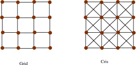
Figure 4: Example of grid graph (left) and cris-cross graph (right) with $n=4$.

Figure 4 shows a lattice or grid graph with $n=4$ (on the left side). There are two scenarios for choosing parameters (with notation $\mathcal{U}[a,b]$ being uniform distribution over interval $[a,b]$):

(1) Varying interaction. $\theta_{i}$ is chosen independently from distribution $\mathcal{U}[-0.05,0.05]$ and $\theta_{ij}$ chosen independent from $\mathcal{U}[-\alpha,\alpha]$ with $\alpha\in\{0.2,0.4,\dots,2\}$.

(2) Varying field. $\theta_{ij}$ is chosen independently from distribution $\mathcal{U}[-0.5,0.5]$ and $\theta_{i}$ chosen independently from $\mathcal{U}[-\alpha,\alpha]$ with $\alpha\in\{0.2,0.4,\dots,2\}$.

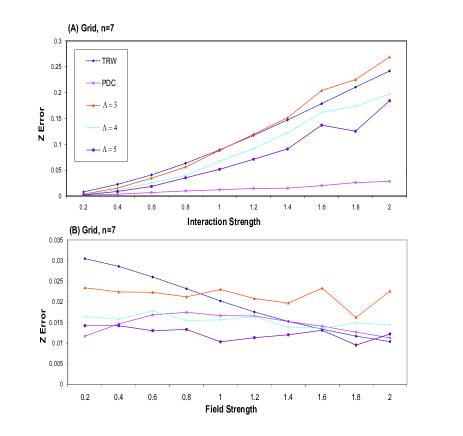
Figure 5: Comparison of TRW, PDC and our algorithm for grid graph with $n=7$ with respect to error in $\log Z$. Our algorithm outperforms TRW and is competitive with respect to PDC.

The grid graph is planar. Hence, we run our algorithms Log Partition  and Mode, with decomposition scheme Minor-e($G,3,{\Lambda}$), ${\Lambda}\in\{3,4,5\}$. We consider two measures to evaluate performance: error in $\log Z$, defined as $\frac{1}{n^{2}}|\log Z^{\text{alg}}-\log Z|$; and error in $\mathbb{E}(\mathbf{x}^{*})$, defined as $\frac{1}{n^{2}}|\mathbb{E}(\mathbf{x}^{\text{alg}}-\mathbb{E}(\mathbf{x}^{*})|$.

We compare our algorithm for error in $\log Z$ with the two recently very successful algorithms – Tree re-weighted algorithm (TRW) and planar decomposition algorithm (PDC). The comparison is plotted in Figure 5 where $n=7$ and results are averages over $40$ trials. The Figure (A) plots error with respect to varying interaction while Figure (B) plots error with respect to varying field strength. Our algorithm, essentially outperforms TRW for these values of ${\Lambda}$ and perform very competitively with respect to PDC.

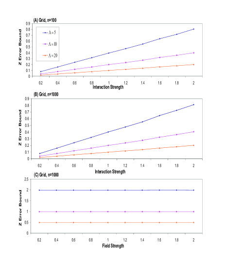
Figure 6: The theoretically computable error bounds for $\log Z$ under our algorithm for grid with $n=100$ and $n=1000$ under varying interaction and varying field model. This clearly shows scalability of our algorithm.

The key feature of our algorithm is scalability. Specifically, running time of our algorithm with a given parameter value ${\Lambda}$ scales linearly in $n$, while keeping the relative error bound exactly the same. To explain this important feature, we plot the theoretically evaluated bound on error in $\log Z$ in Figure 6 with tags (A), (B) and (C). Note that error bound plot is the same for $n=100$ (A) and $n=1000$ (B). Clearly, actual error is likely to be smaller than these theoretically plotted bounds. We note that these bounds only depend on the interaction strengths and not on the values of fields strengths (C).

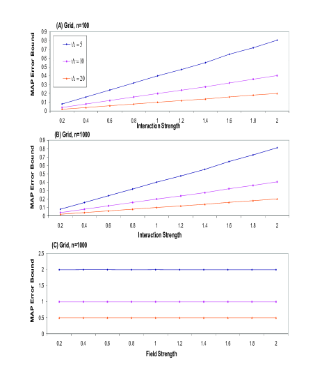
Figure 7: The theoretically computable error bounds for MAP under our algorithm for grid with $n=100$ and $n=1000$ under varying interaction and varying field model.

Results similar to of Log Partition are expected from Mode. We plot the theoretically evaluated bounds on the error in MAP in Figure 7 with tags (A), (B) and (C). Again, the bound on MAP relative error for given ${\Lambda}$ parameter remains the same for all values of $n$ as shown in (A) for $n=100$ and (B) for $n=1000$. There is no change in error bound with respect to the field strength (C).

VII-B Setup 2

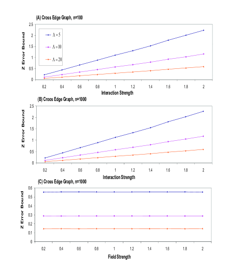
Figure 8: The theoretically computable error bounds for $\log Z$ under our algorithm for cris-cross with $n=100$ and $n=1000$ under varying interaction and varying field model. This clearly shows scalability of our algorithm and robustness to graph structure.

Everything is exactly the same as the above setup with the only difference that grid graph is replaced by cris-cross graph which is obtained by adding extra four neighboring edges per node (exception of boundary nodes). Figure 4 shows cris-cross graph with $n=4$ (on the right side). We again run the same algorithm as above setup on this graph. For cris-cross graph, which is graph with low-doubling dimension, we obtained its graph decomposition from the decomposition of its grid sub-graph. Therefore , the running time of our algorithm remains the same (in order) as that of grid graph and error bound will become only $3$ times weaker than that for the grid graph. We compute these theoretical error bounds for $\log Z$ and MAP which is plotted in Figure 8 and 9. These figures are similar to the Figures 6 and 7 for grid graph.

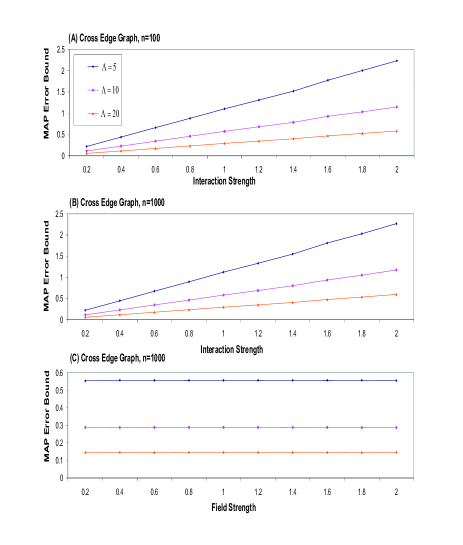
Figure 9: The theoretically computable error bounds for MAP under our algorithm for cris-cross with $n=100$ and $n=1000$ under varying interaction and varying field model.

VIII Unexpected implication: existence of limit

This section describes an important and somewhat unexpected implication of our results, specifically Lemmas 7 and 9. In the context of regular MRF, such as an MRF on $\mathbb{Z}_{n}^{d}$ (of $n^{d}$ nodes) with same node and edge potential functions for all nodes and edges, we will show that (non-trivial) limit $\frac{1}{n^{d}}\log Z$ exists as $n\to\infty$. It is worth noting that showing existence of such limits is not straightforward in general and hence our method should be of interest as such an analytic tool. We believe that the result stated below is well-known; however its proof method is likely to allow for establishing such existence for a more general class of problems. As an example, the theorem will hold even when node and edge potentials are not the same but are chosen from a class of such potential as per some distribution in an i.i.d. fashion. Now, we state the result.

Theorem 8

Consider a regular MRF of $n^{d}$ nodes on $d$-dimensional grid $\mathbb{Z}_{d}^{n}=(V_{n},E_{n})$: let $\psi_{ij}\equiv\psi,\phi_{i}\equiv\phi$ for all $i\in V_{n},(i,j)\in E_{n}$ with $\psi:\Sigma^{2}\to\mathbb{R}_{+},\phi:\Sigma\to\mathbb{R}_{+}$. Let $Z_{n}$ be partition function of this MRF. Then, the following limit exists:

$$\lim_{n\to\infty}\frac{1}{n^{d}}\log Z_{n}=A(d,\phi,\psi)\in(0,\infty).$$

VIII-A Proof of Theorem 8

The proof of Theorem 8 is stated for $d=2$ and $\Sigma=\{0,1\}$ case. Proof for $d\geq 3$ and $\Sigma$ with ${|\Sigma|}\geq 2$ can be proved using exactly the same argument. The proof will use the following Lemmas.

Lemma 12

Let $d=2$ and $\phi^{*}=\max_{\sigma\in\{0,1\}}\phi(\sigma)$, $\psi^{*}=\max_{(\sigma,\sigma^{\prime})\in\{0,1\}^{2}}\psi(\sigma,\sigma^{\prime}).$ Then,

$$n^{2}\leq\log Z_{n}\leq\alpha n^{2},$$

where $\alpha=\log 2+\log\phi^{*}+4\log\psi^{*}$.

Lemma 13

Define $a_{n}=\frac{1}{n^{2}}\log Z_{n}$. Now, given $k>0$, there exists $n(k)$ large enough such that for any $m,n\geq n(k)$,

$$|a_{m}-a_{n}|=O\left(\frac{1}{k}\right)+O\left(\frac{k}{\min{\{{m},{n}}\}}\right).$$

Proof:

(Theorem 8) We state proof of Theorem 8, before proving the above stated Lemmas. First note that, by Lemma 12, the elements of sequence $a_{n}=n^{-2}\log Z_{n}$ take value in $[1,\alpha]$. Now, suppose the claim of theorem is false. That is, sequence $a_{n}$ does not converge as $n\to\infty$. That is, there exists $\delta>0$ such for any choice of $n_{0}$, there are $m\geq n\geq n_{0}$ such that

$$|a_{m}-a_{n}|\geq\delta.$$

By Lemma 13, we can select $k$ large enough and later $n_{0}\geq n(k)$ large enough such that for any $m,n\geq n_{0}$,

$$|a_{m}-a_{n}|<\delta.$$

But this is a contradiction to our assumption that $a_{n}$ does not converge to a limit. That is, we have established that $a_{n}$ converges to a non-trivial limit in $[1,\alpha]$ as desired. This completes the proof of Theorem 8. ∎

VIII-B Proofs of Lemmas

Proof:

(Lemma 12) Consider the following.

$$2^{n^{2}} = \sum_{\mathbf{x}\in\{0,1\}^{n^{2}}}\prod_{i\in V_{n}}1\prod_{(i,j)\in E_{n}}1$$ (26)

$$\stackrel{{\scriptstyle(a)}}{{\leq}} \sum_{\mathbf{x}\in\{0,1\}^{n^{2}}}\prod_{i\in V_{n}}\exp(\phi(x_{i}))\prod_{(i,j)\in E_{n}}\exp(\psi(x_{i},x_{j}))$$

$$= Z_{n}$$

$$\stackrel{{\scriptstyle(b)}}{{\leq}} \sum_{\mathbf{x}\in\{0,1\}^{n^{2}}}\prod_{i\in V_{n}}\exp(\phi^{*})\prod_{(i,j)\in E_{n}}\exp(\psi^{*}).$$

Here, (a) follows from the fact that $\psi,\phi$ are non-negative valued functions and (b) follows from definitions of $\phi^{*},\psi^{*}$. Now, taking logarithm on both sides implies the Lemma 12. ∎

Proof:

(Lemma 13) Given $k>0$, consider $n$ large enough (will be decided later). Consider $\mathbb{Z}_{n}^{2}=(V_{n},E_{n})$ and let it be laid out on $X-Y$ plane so that its node in $V_{n}$ occupy the integral locations : $(i,j),~{}0\leq i\leq n-1,0\leq j\leq n-1$. Now, we describe a scheme to obtain a $(O(1/k),O(k^{2}))$ edge-decomposition of $\mathbb{Z}^{2}_{n}$. For this, choose $\ell_{1},\ell_{2}\in\{0,\dots,k-1\}$ independently and uniformly at random. Select edges to form $\mathcal{B}$ to obtain edge-decomposition as follows: select vertical edges with bottom vertex having $Y$ coordinate $\ell_{2}+jk,j\geq 0$, and select horizontal edges with left vertex having $X$ coordinate $\ell_{1}+jk,j\geq 0$. That is,

$$\mathcal{B} = \{(u,v)\in E_{n}:u=(i,j),v=(i+1,j),i\mbox{~{}mod~{}}k=\ell_{1}\}~{}~{}~{}~{}$$

$$\cup \{(u,v)\in E_{n}:u=(i,j),v=(i,j+1),j\mbox{~{}mod~{}}k=\ell_{2}\}.~{}~{}~{}~{}$$

It is easy to check that this is $(O(1/k),O(k^{2}))$ edge-decomposition due to uniform selection of $\ell_{1},\ell_{2}$ from $\{0,\dots,k-1\}$. Therefore, by Lemma 7, we can obtain estimates that are $(1\pm O(1/k))\log Z_{n}$ using our algorithm.

Let $m=\lceil n/k\rceil$. Under the decomposition $\mathcal{B}$ as described above, there are at least $(m-1)^{2}$ connected components that are MRF on $\mathbb{Z}_{k}$. Also, all the connected components can be covered by at most $(m+1)^{2}$ identical MRFs on $\mathbb{Z}_{k}$. Using arguments similar to those employed in calculations of Theorem 1 (using non-negativity of $\phi,\psi$), it can be shown that the estimate produced by our algorithm is lower bounded as

$$(1-O(1/k))(m-1)^{2}\log Z_{k} = n^{2}\frac{\log Z_{k}}{k^{2}}\times~{}~{}~{}$$

$$\left(1-O(1/k)-O(k/n)\right),~{}~{}~{}$$

and is upper bounded as

$$(1+O(1/k))(m+1)^{2}\log Z_{k} = n^{2}\frac{\log Z_{k}}{k^{2}}\times~{}~{}~{}$$

$$\left(1+O(k/n)+O(1/k)\right).~{}~{}~{}$$

Therefore, from above discussion we obtain that

$$\frac{1}{n^{2}}\log Z_{n}=\frac{Z_{k}}{k^{2}}\left(1\pm O(k/n)\pm O(1/k)\right).$$

Therefore, recalling notation of $a_{n}$, we have that

$$|a_{m}-a_{n}|=a_{k}O\left(\frac{k}{\min{\{m,n\}}}\right)+a_{k}O(1/k).$$

Since, $a_{k}\in[1,\alpha]$ for all $k$, we obtain the desired result of Lemma 13. ∎

IX Conclusion

In this paper, we present simple novel local approximation algorithm for computing log-partition function and MAP estimation for arbitrary exponential distribution represented by a pair-wise MRF. We showed these algorithms provide bounds for arbitrary graph with quantifiable approximation guarantees. Further, for low-doubling dimension graphs and minor-excluded graphs it can provide arbitrary accuracy within linear time. The main takeaway for a practitioner is the following: there is a simple and intuitive local algorithm that provides provable bounds with computable approximation error for any graph and hence it can be used as a good heuristic and producing approximation guarantee certificate.

We proposed message-passing implementation based on self-avoiding walk trees which should provide such implementation for other problems as well. This method, through a transformation from non-binary exponential family to binary MRF, extends for any finite valued factor graph. However, this can result in somewhat redundant construction. Understanding design of direct constructions for non-binary pair-wise MRF is an important open problem.

We derived an unusual implication of our algorithmic results for providing existence of asymptotic limits of free energy for a class of regular MRFs. Our result suggest a way to explicitly evaluate these limiting up to an arbitrary accuracy. This should be of general interest as a method for establishing asymptotic limits as well as computing these limits.

Finally, we remark that our methods are explained for exponential family only. However, they easily extend to certain hard-core models such as independent set or matching where there is a non-constraining assignment to node values.

Appendix A Proof of Lemma 1

The proof is by induction on $r\in\mathbb{N}$. For base case, consider $r=0$. Now, $\mathbf{B}(x,2^{0}=1)$ is essentially the set of all points which are at distance $<1$ by definition. Since it is metric with distance being integer, this means that the set of all points that are at distance $0$. By definition of metric, we have that $x$ is the only such point. That is, $\mathbf{B}(x,1)=\{x\}$. Hence, $|\mathbf{B}(x,1)|=1\leq 2^{0\times\rho(\mathcal{M})}$ for all $x\in\mathcal{X}$.

Now suppose the claim of Lemma is true for all $r\leq k$ and all $x\in\mathcal{X}$. Consider $r=k+1$ and any $x\in\mathcal{X}$. By definition of doubling dimension, there exists $\ell\leq 2^{\rho(\mathcal{M})}$ balls of radius $2^{k}$, say $\mathbf{B}(y_{j},2^{k})$ with $y_{j}\in\mathcal{X}$ for $1\leq j\leq\ell$, such that

$$\mathbf{B}(x,2^{k+1})\subset\cup_{j=1}^{\ell}\mathbf{B}(y_{j},2^{k}).$$

Therefore,

$$|\mathbf{B}(x,2^{k+1})|\leq\sum_{j=1}^{\ell}|\mathbf{B}(y_{j},2^{k})|.$$

By inductive hypothesis, for $1\leq j\leq\ell$,

$$|\mathbf{B}(y_{j},2^{k})|\leq 2^{k\rho(\mathcal{M})}.$$

Since we have $\ell\leq 2^{\rho(\mathcal{M})}$, we obtain

$$|\mathbf{B}(x,2^{k+1})|\leq\ell~{}2^{k\rho(\mathcal{M})}~{}\leq~{}2^{(k+1)\rho(\mathcal{M})}.$$

This completes the proof of inductive step and that of the Lemma 1.

Appendix B Transformation: MAP in factor graph to binary pair-wise MRF

In this section we show that any MAP estimation problem is equivalent to estimating MAP in a specific binary pair-wise problem on a suitably constructed graph with node potentials. This construction is from work by Sanghavi, Shah and Willsky[23]. This construction is related to the “overcomplete basis” representation [2]. Consider the following canonical MAP estimation problem: suppose we are given a distribution $q(\mathbf{y})$ over vectors $\mathbf{y}=(y_{1},\ldots,y_{M})$ of variables $y_{m}$, each of which can take a finite value. Suppose also that $q$ factors into a product of strictly positive functions, which we find convenient to denote in exponential form:

$$q(\mathbf{y})~{}=~{}\frac{1}{Z}\prod_{\alpha\in A}\exp\left(\phi_{\alpha}(\mathbf{y}_{\alpha})\right)~{}=~{}\frac{1}{Z}\exp\left(\sum_{\alpha\in A}\phi_{\alpha}(\mathbf{y}_{\alpha})\right)$$

Here $\alpha$ specifies the domain of the function $\phi_{\alpha}$, and $\mathbf{y}_{\alpha}$ is the vector of those variables that are in the domain of $\phi_{\alpha}$. The $\alpha$’s also serve as an index for the functions. $A$ is the set of functions. The MAP estimation problem is to find a maximizing assignment $\mathbf{y}^{*}\in\arg\max_{\mathbf{y}}q(\mathbf{y})$.

We now build an auxillary graph $\widetilde{G}$, and assign weights to its nodes, such that the MAP estimation problem above is equivalent to finding the MWIS of $\widetilde{G}$. There is one node in $\widetilde{G}$ for each pair $(\alpha,\mathbf{y}_{\alpha})$, where $\mathbf{y}_{\alpha}$ is an assignment (i.e. a set of values for the variables) of domain $\alpha$. We will denote this node of $\widetilde{G}$ by $\delta(\alpha,\mathbf{y}_{\alpha})$.

There is an edge in $\widetilde{G}$ between any two nodes $\delta(\alpha_{1},\mathbf{y}_{\alpha_{1}}^{1})$ and $\delta(\alpha_{2},\mathbf{y}_{\alpha_{2}}^{2})$ if and only if there exists a variable index $m$ such that

1. $m$ is in both domains, i.e. $m\in\alpha_{1}$ and $m\in\alpha_{2}$, and

2. the corresponding variable assignments are different, i.e. $y^{1}_{m}\neq y^{2}_{m}$.

In other words, we put an edge between all pairs of nodes that correspond to inconsistent assignments. Given this graph $\widetilde{G}$, we now assign weights to the nodes. Let $c>0$ be any number such that $c+\phi_{\alpha}(\mathbf{y}_{\alpha})>0$ for all $\alpha$ and $\mathbf{y}_{\alpha}$. The existence of such a $c$ follows from the fact that the set of assignments and domains is finite. Assign to each node $\delta(\alpha,\mathbf{y}_{\alpha})$ a weight of $c+\phi_{\alpha}(\mathbf{y}_{\alpha})$. Consider an example of this construction first. Later, we state the precise equivalence.

Figure 10: Example of transforming MAP for factor graph to MAP in binary pair-wise MRF.

Example 2

Let $y_{1}$ and $y_{2}$ be binary variables with joint distribution

$$q(y_{1},y_{2})~{}=~{}\frac{1}{Z}\exp(\theta_{1}y_{1}+\theta_{2}y_{2}+\theta_{12}y_{1}y_{2})$$

where the $\theta$ are any real numbers. The corresponding $\widetilde{G}$ is shown in Figure 10. Let $c$ be any number such that $c+\theta_{1}$, $c+\theta_{2}$ and $c+\theta_{12}$ are all greater than 0. The weights on the nodes in $\widetilde{G}$ are: $\theta_{1}+c$ on node “1” on the left, $\theta_{2}+c$ for node “1” on the right, $\theta_{12}+c$ for the node “11”, and $c$ for all the other nodes.

Lemma 14

Suppose $q$ and $\widetilde{G}$ are as above. (a) If $\mathbf{y}^{*}$ is a MAP estimate of $q$, let $\delta^{*}=\{\delta(\alpha,\mathbf{y}^{*}_{\alpha})\,|\,\alpha\in A\}$ be the set of nodes in $\widetilde{G}$ that correspond to each domain being consistent with $\mathbf{y}^{*}$. Then, $\delta^{*}$ is an MWIS of $\widetilde{G}$. (b) Conversely, suppose $\delta^{*}$ is an MWIS of $\widetilde{G}$. Then, for every domain $\alpha$, there is exactly one node $\delta(\alpha,\mathbf{y}^{*}_{\alpha})$ included in $\delta^{*}$. Further, the corresponding domain assignments$\{\mathbf{y}^{*}_{\alpha}\,|\,\alpha\in A\}$ are consistent, and the resulting overall vector $\mathbf{y}^{*}$ is a MAP estimate of $q$.

Proof:

A maximal independent set is one in which every node is either in the set, or is adjacent to another node that is in the set. Since weights are positive, any MWIS has to be maximal. For $\widetilde{G}$ and $q$ as constructed, it is clear that

1. If $\mathbf{y}$ is an assignment of variables, consider the corresponding set of nodes $\{\delta(\alpha,\mathbf{y}_{\alpha})\,|\,\alpha\in A\}$. Each domain $\alpha$ has exactly one node in this set. Also, this set is an independent set in $\widetilde{G}$, because the partial assignments $\mathbf{y}_{\alpha}$ for all the nodes are consistent with $\mathbf{y}$, and hence with each other. This means that there will not be an edge in $\widetilde{G}$ between any two nodes in the set.

2. Conversely, if $\Delta$ is a maximal independent set in $\widetilde{G}$, then all the sets of partial assignments corresponding to each node in $\Delta$ are all consistent with each other, and with a global assignment $\mathbf{y}$.

There is thus a one-to-one correspondence between maximal independent sets in $\widetilde{G}$ and assignments $\mathbf{y}$. The lemma follows from this observation. ∎

References

• [1] J. Pearl, Probabilistic Reasoning in Intelligent Systems: Networks of Plausible Inference.   San Francisco, CA: Morgan Kaufmann, 1988.
• [2] M. Wainwright and M. Jordan, “Graphical models, exponential families, and variational inference,” UC Berkeley, Dept. of Statistics, Technical Report 649, 2003.
• [3] A. Sinclair and M. Jerrum, “Approximate counting, uniform generation and rapidly mixing markov chains,” Inf. Comput., vol. 82, no. 1, pp. 93–133, 1989.
• [4] F. P. Kelly, “Loss networks,” Annals of Applied Probability, vol. 1, pp. 319–378, 1991.
• [5] J. Yedidia, W. Freeman, and Y. Weiss, “Generalized belief propagation,” Mitsubishi Elect. Res. Lab., TR-2000-26, 2000.
• [6] M. J. Wainwright, T. Jaakkola, and A. S. Willsky, “Tree-based reparameterization framework for analysis of sum-product and related algorithms,” IEEE Transactions on Information Theory, 2003.
• [7] ——, “Map estimation via agreement on (hyper)trees: Message-passing and linear-programming approaches,” IEEE Transactions on Information Theory, 2005.
• [8] ——, “A new class of upper bounds on the log partition function,” IEEE Transactions on Information Theory, 2005.
• [9] S. C. Tatikonda and M. I. Jordan, “Loopy belief propagation and gibbs measure,” in Uncertainty in Artificial Intelligence, 2002.
• [10] M. Bayati, D. Shah, and M. Sharma, “Max-product for maximum weight matching: convergence, correctness and lp duality,” IEEE Transaction on Information Theory, Accepted, preliminary version appeared in IEEE, ISIT 2005.
• [11] C. Moallemi and B. V. Roy, “Convergence of the min-sum message passing algorithm for quadratic optimization,” Stanford University Technical report, 2006.
• [12] V. Kolmogorov and M. Wainwright, “On optimality of tree-reweighted max-product message-passing,” in Uncertainty in Artificial Intelligence, 2005.
• [13] V. Kolmogorov, “Convergent tree-reweighted message passing for energy minimization,” IEEE Transactions on Pattern Analysis and Machine Intelligence, 2006.
• [14] A. Globerson and T. Jaakkola, “Bound on partition function through planar graph decomposition,” in NIPS, 2006.
• [15] P. Klein, S. Plotkin, and S. Rao, “Excluded minors, network decomposition and multicommodity flow,” in ACM STOC, 1993.
• [16] S. Rao, “Small distortion and volume preserving embeddings for planar and euclidean metrics,” in SCG ’99: Proceedings of the fifteenth annual symposium on Computational geometry.   New York, NY, USA: ACM Press, 1999, pp. 300–306.
• [17] N. Madras and G. Slade, The Self-Avoiding Walk.   Birkhauser, Boston, 1993.
• [18] D. Weitz, “Counting independent sets up to the tree threshold,” in STOC ’06: Proceedings of the thirty-eighth annual ACM symposium on Theory of computing.   New York, NY, USA: ACM Press, 2006, pp. 140–149.
• [19] D. R. Karger and M. Ruhl, “Finding nearest neighbors in growth-restricted metrics,” in STOC ’02: Proceedings of the thiry-fourth annual ACM symposium on Theory of computing.   New York, NY, USA: ACM Press, 2002, pp. 741–750.
• [20] A. Gupta, R. Krauthgamer, and J. R. Lee, “Bounded geometries, fractals, and low-distortion embeddings,” in FOCS ’03: Proceedings of the 44th Annual IEEE Symposium on Foundations of Computer Science.   Washington, DC, USA: IEEE Computer Society, 2003, p. 534.
• [21] S. Har-Peled and S. Mazumdar, “On coresets for k-means and k-median clustering,” in STOC ’04: Proceedings of the thirty-sixth annual ACM symposium on Theory of computing.   New York, NY, USA: ACM Press, 2004, pp. 291–300.
• [22] N. Robertson and P. Seymour, “The graph minor theory,” started, 1984.
• [23] S. Sanghavi, D. Shah, and A. Willsky, “Max-product for maximum weight independent set,” Pre-print, 2007.