Robust De-anonymization of Large Datasets
(How to Break Anonymity of the Netflix Prize Dataset)

Abstract

We present a new class of statistical de-anonymization attacks against high-dimensional micro-data, such as individual preferences, recommendations, transaction records and so on. Our techniques are robust to perturbation in the data and tolerate some mistakes in the adversary’s background knowledge.

We apply our de-anonymization methodology to the Netflix Prize dataset, which contains anonymous movie ratings of 500,000 subscribers of Netflix, the world’s largest online movie rental service. We demonstrate that an adversary who knows only a little bit about an individual subscriber can easily identify this subscriber’s record in the dataset. Using the Internet Movie Database as the source of background knowledge, we successfully identified the Netflix records of known users, uncovering their apparent political preferences and other potentially sensitive information.

1 Introduction

Datasets containing “micro-data,” that is, information about specific individuals, are increasingly becoming public—both in response to “open government” laws, and to support data mining research. Some datasets include legally protected information such as health histories; others contain individual preferences, purchases, and transactions, which many people may view as private or sensitive.

Privacy risks of publishing micro-data are well-known. Even if identifying information such as names, addresses, and Social Security numbers has been removed, the adversary can use contextual and background knowledge, as well as cross-correlation with publicly available databases, to re-identify individual data records. Famous re-identification attacks include de-anonymization of a Massachusetts hospital discharge database by joining it with with a public voter database [22], de-anonymization of individual DNA sequences [19], and privacy breaches caused by (ostensibly anonymized) AOL search data [12].

Micro-data are characterized by high dimensionality and sparsity. Informally, micro-data records contain many attributes, each of which can be viewed as a dimension (an attribute can be thought of as a column in a database schema). Sparsity means that a pair of random records are located far apart in the multi-dimensional space defined by the attributes. This sparsity is empirically well-established [6, 4, 16] and related to the “fat tail” phenomenon: individual transaction and preference records tend to include statistically rare attributes.

Our contributions. We present a very general class of statistical de-anonymization algorithms which demonstrate the fundamental limits of privacy in public micro-data. We then show how these methods can be used in practice to de-anonymize the Netflix Prize dataset, a 500,000-record public dataset.

Our first contribution is a rigorous formal model for privacy breaches in anonymized micro-data (section 3). We present two definitions, one based on the probability of successful de-anonymization, the other on the amount of information recovered about the target. Unlike previous work [22], we do not assume a priori that the adversary’s knowledge is limited to a fixed set of “quasi-identifier” attributes. Our model thus encompasses a much broader class of de-anonymization attacks than simple cross-database correlation.

Our second contribution is a general de-anonymization algorithm (section 4). Under very mild assumptions about the distribution from which the records are drawn, the adversary with a small amount of background knowledge about an individual can use it to identify, with high probability, this individual’s record in the anonymized dataset and to learn all anonymously released information about him or her, including sensitive attributes. For sparse datasets, such as most real-world datasets of individual transactions, preferences, and recommendations, very little background knowledge is needed (as few as 5-10 attributes in our case study). Our de-anonymization algorithm is robust to imprecision of the adversary’s background knowledge and to sanitization or perturbation that may have been applied to the data prior to release. It works even if only a subset of the original dataset has been published.

Our third contribution is a practical analysis of the Netflix Prize dataset, containing anonymized movie ratings of 500,000 Netflix subscribers (section 5). Netflix—the world’s largest online movie rental service—published this dataset to support the Netflix Prize data mining contest. We demonstrate that an adversary who knows only a little bit about an individual subscriber can easily identify his or her record if it is present in the dataset, or, at the very least, identify a small set of records which include the subscriber’s record. The adversary’s background knowledge need not be precise, e.g., the dates may only be known to the adversary with a 14-day error, the ratings may be known only approximately, and some of the ratings and dates may even be completely wrong. Because our algorithm is robust, if it uniquely identifies a record in the published dataset, with high probability this identification is not a false positive, even though the dataset contains the records of only $\frac{1}{8}$ of all Netflix subscribers (as of the end of 2005, which is the “cutoff” date of the dataset),

2 Related work

Unlike statistical databases [26, 1, 3, 7, 5], micro-data datasets contain actual records of individuals even after anonymization. A popular approach to micro-data privacy is $k$-anonymity [24, 23, 8]. The data publisher must determine in advance which of the attributes are available to the adversary (these are called “quasi-identifiers”), and which are the “sensitive attributes” to be protected. $k$-anonymization ensures that each “quasi-identifier” tuple occurs in at least $k$ records in the anonymized database. It is well-known that $k$-anonymity does not guarantee privacy, because the values of sensitive attributes associated with a given quasi-identifier may not be sufficiently diverse [17, 18] or because the adversary has access to background knowledge [17]. Mere knowledge of the $k$-anonymization algorithm may be sufficient to break privacy [27]. Furthermore, $k$-anonymization completely fails on high-dimensional datasets [2], such as the Netflix Prize dataset and most real-world datasets of individual recommendations and purchases.

In contrast to previous attacks on micro-data privacy [22], our de-anonymization algorithm does not assume that the attributes are divided a priori into quasi-identifiers and sensitive attributes. Examples include anonymized transaction records (if the adversary knows a few of the individual’s purchases, can he learn all of her purchases?), recommendation and rating services (if the adversary knows a few movies that the individual watched, can he learn all movies she watched?), Web browsing and search histories [12], and so on. In such datasets, it is impossible to tell in advance which attributes might be available to the adversary; the adversary’s background knowledge may even vary from individual to individual. Unlike [22, 19, 10], our algorithm is robust. It works even if the published records have been perturbed, if only a subset of the original dataset has been published, and if there are mistakes in the adversary’s background knowledge.

Our main case study is the Netflix Prize dataset of movie ratings. We are aware of only one previous paper that considered privacy of movie ratings. In collaboration with the MovieLens recommendation service, Frankowski et al. correlated public mentions of movies in the MovieLens discussion forum with the users’ movie rating histories in the internal MovieLens dataset [10]. The algorithm uses the entire public record as the background knowledge (29 ratings per user, on average), and is not robust if this knowledge is imprecise (e.g., if the user publicly mentioned movies which he did not rate).

By contrast, our analysis is based solely on public data. Our de-anonymization is not based on cross-correlating Netflix internal datasets (to which we do not have access) with public Netflix forums. It requires much less background knowledge (2-8 ratings per user), which need not be precise. Furthermore, our analysis has privacy implications for 500,000 Netflix subscribers whose records have been published; by contrast, the largest public MovieLens datasets contains only 6,000 records.

3 Model

Database. Define database ${\cal D}$ to be an $N\times M$ matrix where each row is a record associated with some individual, and the columns are attributes. We are interested in databases containing individual preferences and transactions, such as shopping histories, movie or book preferences, Web browsing histories, and so on. Thus, the number of columns reflects the total number of items in the space we are considering, ranging from a few thousands for movies to millions for (say) the amazon.com catalog.

Each attribute (column) can be thought of as a dimension, and each individual record as a point in the multidimensional attribute space. To keep our analysis general, we will not fix the space $X$ from which attributes are drawn. They may be boolean (e.g., has this book been rated), integer (e.g., the book’s rating on a 1-10 scale), date, or a tuple such as a (rating, date) pair.

The typical reason to publish anonymized databases is “collaborative filtering,” i.e., predicting a customer’s future choices from his past behavior using the knowledge of what similar customers did. Abstractly, the goal is to predict the value of some attributes using a combination of other attributes. This is used in shopping recommender systems, aggressive caching in Web browsers, and so on [25].

Sparsity and similarity. Preference databases with thousands to millions of attributes are necessarily sparse, i.e., each individual record contains values only for a small fraction of attributes. We call these non-null attributes, and the set of non-null attributes the support of a record (denoted $\textsf{supp}(r)$). Null attributes are denoted $\perp$. The support of a column is defined analogously. For example, the shopping history of even the most profligate Amazon shopper contains only a tiny fraction of all available items. Even though points corresponding to database records are very sparse in the attribute space, each record may have dozens or hundreds of non-null attributes, making the database truly high-dimensional.

The distribution of support sizes of attributes is typically heavy- or long-tailed, roughly following the power law [6, 4]. This means that although the supports of the columns corresponding to “unpopular” items are small, these items are so numerous that they make up the bulk of the non-null entries in the database. Thus, any attempt to approximate the database by projecting it down to the most common columns is bound to failure. (The same effect causes $k$-anonymization to completely fail on such databases [2].)

Unlike “quasi-identifiers” [24, 8], each attribute typically has very little entropy for de-anonymization purposes. In a large database, for any except the rarest attributes, there are hundreds of records with the same value of this attribute as any given record. Therefore, it is not a quasi-identifier. At the same time, knowledge that a particular individual has a certain attribute value does reveal some information about her record, since attribute values and even the mere fact that the attribute is non-null vary from record to record.

The similarity measure Sim is a function that maps a pair of attributes (or more generally, a pair of records) to the interval $[0,1]$. It captures the intuitive notion of two values being “similar.” Typically, Sim on attributes will behave like a delta function. For example, in our analysis of the Netflix Prize dataset, Sim outputs 1 on a pair of movies rated by different subscribers if and only if both the ratings and the dates are within a certain threshold of each other (otherwise it outputs 0).

To define Sim over two records $r_{1},r_{2}$, we “generalize” the cosine similarity measure:

$$\textsf{Sim}(r_{1},r_{2})=\frac{\sum\textsf{Sim}(r_{1i},r_{2i})}{|\textsf{supp}(r_{1})\cup\textsf{supp}(r_{2})|}$$

Definition 1 (Sparsity)

A database $D$ is $(\epsilon,\delta)$-sparse w.r.t. the similarity measure Sim if

$$\Pr_{r}[\textsf{Sim}(r,r^{\prime})>\epsilon\ \forall r^{\prime}\neq r]\leq\delta$$

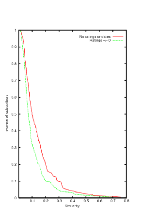
As a real-world example, in appendix E we show that the Netflix Prize dataset is overwhelmingly sparse: for the vast majority of records, there isn’t a single similar record in the entire 500,000-record dataset.

Sanitization and sampling. Our de-anonymization algorithms are designed to work against databases that have been anonymized and “sanitized” by their publishers. The three main sanitization methods are perturbation, generalization, and suppression [23, 8]. Furthermore, the data publisher may only release a (possibly non-uniform) sample of the database. For example, he may attempt to $k$-anonymize the records, and then release only one record out of each cluster of $k$ or more records.

If the database is released for collaborative filtering or similar data mining purposes (as in the case of the Netflix Prize dataset), the “error” introduced by sanitization cannot be large, otherwise its utility will be lost. We make this precise in our analysis. Our definition of privacy breach (see below) allows the adversary to identify not just his target’s record, but any record as long as it is sufficiently similar (via Sim) to the target and can thus be used to determine its attributes with high probability.

From the viewpoint of our algorithm, there is no difference between the perturbation of the published records and the imprecision of the adversary’s knowledge about his target. In both cases, there is a small discrepancy between an attribute value in the target’s anonymous record and her attribute value as known to the adversary. Our de-anonymization algorithm is designed to be robust to both. Therefore, in the rest of the paper we will treat perturbation applied to the data simply as imprecision of the adversary’s knowledge, and assume that the public, anonymized sample ${\hat{D}}$ is an (arbitrary, unless otherwise specified) subset of $D$.

Adversary model. The adversary’s goal is to de-anonymize an anonymous record $r$ from the public database. To model this formally, we sample $r$ randomly from $D$ and give a little bit of auxiliary information or background knowledge related to $r$ to the adversary. It is restricted to a subset of the (possibly imprecise, perturbed, or simply incorrect) values of $r$’s attributes, modeled as an arbitrary probabilistic function $\textsf{Aux}\colon X^{M}\rightarrow X^{M}$. The attributes given to the adversary may be chosen uniformly from the support of $r$, or according to some other probability distribution. Given this auxiliary information and an anonymized sample of the database, the adversary’s goal is to reconstruct attribute values of the entire record $r$.

In $k$-anonymity, there is a rigid division between demographic quasi-identifiers and sensitive medical attributes (none of which are known to the adversary) [24]. By contrast, in our model if the adversary happens to know the value of some attribute for his target, it becomes part of his auxiliary information and thus an “identifier” (but only for this individual’s record). If revealing the value of some attribute violates some individual’s privacy (this depends on the specific record), then it is “sensitive” for this individual.

Privacy breach: formal definitions. What does it mean to de-anonymize a record $r$? The naive answer is to find the “right” anonymized record in the public sample ${\hat{D}}$. This is hard to capture formally, however, because it requires assumptions about the data publishing process (e.g., what if ${\hat{D}}$ contains two copies of every original record?). Fundamentally, the adversary’s objective is privacy breach: he wants to learn as much as he can about $r$’s attributes that he doesn’t already know. We give two different (but related) formal definitions, because there are two distinct scenarios for privacy breaches in large databases.

The first scenario is automated large-scale de-anonymization. For every record $r$ about which he has some information, the adversary must produce a single “prediction” for all attributes of $r$. An example is the attack that inspired $k$-anonymity [22]: taking the demographic data from a voter database as auxiliary information, the adversary joins it with the anonymized hospital discharge database and uses the resulting combination to determine the values of medical attributes for each person who appears in both databases.

Definition 2

A database $D$ can be $(\theta,\omega)$-deanonymized w.r.t. auxiliary information Aux if there exists an algorithm $A$ which, on inputs $D$ and $\textsf{Aux}(r)$ where $r\leftarrow D$ outputs $r^{\prime}$ such that

$$\Pr[\textsf{Sim}(r,r^{\prime})\geq\theta]\geq\omega$$

Definition 2 can be interpreted as an amplification of background knowledge: the adversary starts with $\textsf{aux}=\textsf{Aux}(r)$ which is close to $r$ on a small subset of attributes, and uses this to compute $r^{\prime}$ which is close to $r$ on the entire set of attributes. This captures the adversary’s ability to gain information about his target record. He does not need to precisely identify the “right” anonymized record (as we argue above, this notion may be meaningless). As long the adversary finds some record which is guaranteed to be very similar to the target record, i.e., contains the same or similar attribute values, privacy breach has occurred.

If operating on a sample of the entire database, the de-anonymization algorithm must also detect whether its target record is part of the sample, or has not been released at all. In the following, the probability is taken over the randomness of the sampling of $r$ from ${\hat{D}}$, Aux and $A$ itself.

Definition 3 (De-anonymization)

An arbitrary subset ${\hat{D}}$ of a database $D$ can be $(\theta,\omega)$-deanonymized w.r.t. auxiliary information Aux if there exists an algorithm $A$ which, on inputs ${\hat{D}}$ and $\textsf{Aux}(r)$ where $r\leftarrow D$

• If $r\in{\hat{D}}$, outputs $r^{\prime}$ s.t. $\Pr[\textsf{Sim}(r,r^{\prime})\geq\theta]\geq\omega$

• if $r\notin{\hat{D}}$, outputs $\perp$ with probability at least $\omega$

The same error threshold ($1-\omega$) is used for both “failures”–false positives and false negatives–in the above definition because the parameters of the algorithm can be adjusted so that both rates are equal; this is the so called “equal error rate.”

In the second privacy breach scenario, the adversary produces a set or “lineup” of candidate records that include his target record $r$, either because there is not enough auxiliary information to identify $r$ in the lineup or because he expects to perform additional, possibly manual analysis to complete de-anonymization. This is similar to communication anonymity in mix networks [21].

The number of candidate records is not a good metric, because some of the records may be much likelier candidates than others. Instead, we consider the probability distribution over the candidate records, and use the conditional entropy of $r$ given aux as the metric. In the absence of an “oracle” to identify the target record $r$ in the lineup, the entropy of the distribution itself can be used as a metric [21, 9]. If the adversary has such an “oracle” (this is a technical device used to measure the adversary’s success; in the real world, the adversary may not have an oracle telling him whether de-anonymization succeeded), then privacy breach can be quantified by answering a very specific question: how many bits of additional information does the adversary need in order to output a record which is similar to his target record?

Thus, suppose that after executing the de-anonymization algorithm, the adversary outputs records $r^{\prime}_{1},\ldots r^{\prime}_{k}$ and the coresponding probabilities $p_{1},\ldots p_{k}$. The latter can be viewed as an entropy encoding of the candidate records. According to Shannon’s source coding theorem, the optimal code length for record $r^{\prime}_{i}$ is $-\log p_{i}$. We denote by $H_{S}(\Pi,x)$ this Shannon entropy of a record $x$ w.r.t. a probability distribution $\Pi$. In the following, the expectation is taken over the coin tosses of $A$, the sampling of $r$ and Aux.

Definition 4 (Entropic de-anonymization)

A database $D$ can be $(\theta,H)$-deanonymized w.r.t. auxiliary information Aux if there exists an algorithm $A$ which, on inputs $D$ and $\textsf{Aux}(r)$ where $r\leftarrow D$ outputs a set of candidate records $D^{\prime}$ and probability distribution $\Pi$ such that

$$E[\textsf{min}_{r^{\prime}\in D^{\prime},\textsf{Sim}(r,r^{\prime})\geq\theta}H_{S}(\Pi,r^{\prime})]\leq H$$

This definition measures the minimum Shannon entropy of the candidate set of records which are similar to the target record. As we will show, in sparse databases this set is likely to contain a single record, thus taking the minimum is but a syntactic requirement.

When the minimum is taken over an empty set, we define it to be $H_{0}=\log_{2}N$, the a priori entropy of the target record. Intuitively, this models the adversary outputting a random record from the entire database when he cannot compute a lineup of plausible candidates. Formally, the adversary’s algorithm $A$ can be converted into an algorithm $A^{\prime}$, which outputs the mean of two probability distributions: one is the output of $A$, the other is the uniform distribution over $D$. Observe that for $A^{\prime}$, the minimum is always taken over a non-empty set, and the expectation for $A^{\prime}$ differs from that for $A$ by at most 1 bit.

4 De-anonymization algorithm

We start by describing a meta-algorithm or an algorithm template. The inputs are a sample ${\hat{D}}$ of database $D$ and auxiliary information $\textsf{aux}=Aux(r),r\leftarrow D$. The output is either a record $r^{\prime}\in{\hat{D}}$, or a set of candidate records and a probability distribution over those records (following Definitions 3 and 4, respectively). The three main components of the algorithm are the scoring function, matching criterion, and record selection.

The scoring function Score assigns a numerical score to each record in ${\hat{D}}$ based on how well it matches the adversary’s auxiliary information Aux. The matching criterion is the algorithm that the adversary applies to the set of scores assigned by the scoring function to determine if there is a match. Finally, record selection selects one “best-guess” record or a probability distribution, if needed.

The template for the de-anonymization algorithm is as follows:

1. The adversary computes $\textsf{Score}(\textsf{aux},r^{\prime})$ for each $r^{\prime}\in{\hat{D}}$.

2. The adversary applies the matching criterion to the resulting set of scores and computes the matching set; if the matching set is empty, the adversary outputs $\perp$ and exits. (This step can be skipped if ${\hat{D}}=D$, i.e., if the entire database has been released, or if the adversary knows for certain that the target record has been released, i.e., $r\in{\hat{D}}$).

3. If the adversary’s “best guess” is required (de-anonymization according to Definitions 2 and 3), the adversary outputs $r^{\prime}\in{\hat{D}}$ with the highest score. If a probability distribution over candidate records is required (de-anonymization according to Definition 4), the adversary computes some non-decreasing probability distribution based on the score and outputs this distribution.

Algorithm 1A. The following simple instantiation of the above algorithm template is sufficiently tractable to be formally analyzed in the rest of this section.

• $\textsf{Score}(\textsf{aux},r^{\prime})=\textsf{min}_{i\in\textsf{supp}(\textsf{aux})}\textsf{Sim}(\textsf{aux}_{i},r^{\prime}_{i})$, i.e., the score of a candidate record is determined by the least similar attribute between it and the adversary’s knowledge.

• The adversary computes the matching set $D^{\prime}=\{r^{\prime}\in{\hat{D}}:\textsf{Score}(\textsf{aux},r^{\prime})>\alpha\}$ for some fixed constant $\alpha$. The matching criterion is that $D^{\prime}$ be nonempty.

• Probability distribution is uniform on $D^{\prime}$.

Algorithm 1B. This algorithm incorporates several heuristics which have proved useful in practical analysis (see section 5). First, the scoring function gives higher weight to statistically rare attributes. The intuition is as follows: if the auxiliary information tells the adversary that his target has a certain rare attribute, this contains much more information for de-anonymization purposes than the knowledge of a common attribute (e.g., it is more useful to know that the target has purchased “The Dedalus Book of French Horror” than the fact that she purchased a Harry Potter book).

Second, to improve robustness of the algorithm, the matching criterion requires that the top score be significantly above the second-best score. This measures how much the identified record “stands out” from other candidate records.

• $\textsf{Score}(\textsf{aux},r^{\prime})=\sum_{i\in\textsf{supp}(\textsf{aux})}\textsf{wt}(i)\textsf{Sim}(\textsf{aux}_{i},r^{\prime}_{i})$ where $\textsf{wt}(i)=\frac{1}{\log|\textsf{supp}(i)|}$.

• The adversary computes $\textsf{max}=\textsf{max}(S),\textsf{max}_{2}=\textsf{max}_{2}(S)$ and $\sigma=\sigma(S)$ where $S=\{\textsf{Score}(\textsf{aux},r^{\prime}):r^{\prime}\in{\hat{D}}\}$, i.e., the highest and second-highest scores and the standard deviation of the scores. If $\frac{\textsf{max}-\textsf{max}_{2}}{\sigma}<\phi$, where $\phi$ is a fixed parameter called the eccentricity, then there is no match; otherwise, the matching set consists of the record with the highest score.

• Probability distribution is $\Pi(r^{\prime})=c\cdot e^{\frac{\textsf{Score}(\textsf{aux},r^{\prime})}{\sigma}}$ for each $r^{\prime}$, where $c$ is a constant that makes the distribution sum up to 1. This weighs each matching record in inverse proportion to the likelihood that the match in question is a statistical fluke.

4.1 Analysis: general case

We now quantify the amount of auxiliary information needed to de-anonymize an arbitrary multi-dimensional dataset using our Algorithm 1A. The smaller the required auxiliary information (i.e., the fewer attribute values the adversary needs to know about his target), the easier the attack.

We start with the worst-case analysis and calculate how much auxiliary information is needed in the most general case, without any assumptions about the distribution from which the data are drawn. In section 4.2, we will show that much less auxiliary information is needed to de-anonymize records drawn from sparse distributions (all known real-world examples of transactions and recommendation datasets are sparse).

Let aux be the auxiliary information about some record $r$ from the dataset. This knowledge consists of $m$ (non-null) attribute values, which are close to the corresponding values of attributes in $r$, that is, $|\textsf{aux}|=m$ and $\textsf{Sim}(\textsf{aux}_{i},r_{i})\geq 1-\epsilon\ \forall i\in\textsf{supp}(\textsf{aux})$, where $\textsf{aux}_{i}$ (respectively, $r_{i}$) is the $i$th attribute of aux (respectively, $r$).

Theorem 1

Let $0<\epsilon,\delta<1$ and let $D$ be the database. Let Aux be such that $\textsf{aux}=\textsf{Aux}(r)$ consists of at least $m\geq\frac{\log N-\log\epsilon}{-\log(1-\delta)}$ randomly selected attribute values of the target record $r$, with $\textsf{Sim}(\textsf{aux}_{i},r_{i})\geq 1-\epsilon\ \forall i\in\textsf{supp}(\textsf{aux})$. Then $D$ can be $(1-\epsilon-\delta,1-\epsilon)$-deanonymized w.r.t. Aux.

Proof. The adversary uses Algorithm 1A with $\alpha=1-\epsilon$ to compute the set of all records in ${\hat{D}}$ that match aux. The adversary then outputs a record $r^{\prime}$ at random from the matching set. It is sufficient to prove that this randomly chosen $r^{\prime}$ must be very similar to the target record $r$. (This satisfies our definition of a privacy breach because it gives to the adversary almost everything he may want to learn about $r$.)

Record $r^{\prime}$ is a false match if $\textsf{Sim}(r,r^{\prime})\leq 1-\epsilon-\delta$ (i.e., the likelihood that it is similar to the target record $r$ is below the threshold). We first show that, with high probability, the matching set does not contain any false matches.

Lemma 1

If $r^{\prime}$ is a false match, then $\Pr_{i\in\textsf{supp}(r)}[\textsf{Sim}(r_{i},r_{i}^{\prime})\geq 1-\epsilon]<1-\delta$

Lemma 1 holds, because the contrary implies $\textsf{Sim}(r,r^{\prime})\geq(1-\epsilon)(1-\delta)\geq(1-\epsilon-\delta)$, contradicting the assumption that $r^{\prime}$ is a false match. Therefore, the probability that the false match $r^{\prime}$ belongs to the matching set is at most $(1-\delta)^{m}$. By a union bound, the probability that there is even a single false match $r^{\prime}$ in the matching set is at most $N(1-\delta)^{m}$. If $m=\frac{\log\frac{N}{\epsilon}}{\log\frac{1}{1-\delta}}$, then the probability that the matching set returned by Algorithm 1A contains any false matches is no more than $\epsilon$.

Therefore, with probability $1-\epsilon$, there are no false matches. Thus for every record $r^{\prime}$ in the matching set, $\textsf{Sim}(r,r^{\prime})\geq 1-\epsilon-\delta$, i.e., any $r^{\prime}$ must be similar to the true record $r$. To complete the proof, observe that the matching set contains at least one record, $r$ itself.

When $\delta$ is small, $m=\frac{\log N-\log\epsilon}{\delta}$. Note the logarithmic dependence on $\epsilon$ and the linear dependence on $\delta$: the chance that the de-anonymization algorithm completely fails is very small even if attribute-wise accuracy is not very high. Also note that the size of the matching set need not be small. Even if the de-anonymization algorithm returns a large number of records, with high probability they are all similar to the target record $r$, and thus any one of them can be used to learn the unknown sensitive attributes of $r$.

4.2 Analysis: sparse datasets

As shown in section 3, most real-world datasets containing individual transactions, preferences, and so on are sparse. Sparsity increases the probability that de-anonymization succeeds, decreases the amount of auxiliary information needed, and makes the algorithm more robust to both perturbation in the data and mistakes in the auxiliary information.

Our assumptions about data sparsity are very mild. We only assume $(1-\epsilon-\delta,\ldots)$ sparsity, i.e., we assume that the average record does not have extremely similar peers in the dataset (real-world records tend not to have even approximately similar peers—see appendix E).

Theorem 2

Let $\epsilon$, $\delta$, and aux be as in Theorem 1. If the database $D$ is $(1-\epsilon-\delta,\epsilon)$-sparse, then $D$ can be $(1,1-\epsilon)$-deanonymized. $\Box$

The proof is essentially the same as the proof of Theorem 1, but in this case any $r^{\prime}\neq r$ from the matching set must be a false match. Because with probability $1-\epsilon$, Algorithm 1A outputs no false matches, the matching set consists of exactly one record: the true target record $r$.

Finally, de-anonymization in the sense of Definition 4 requires even less auxiliary information. Recall that in this kind of privacy breach, the adversary outputs a “lineup” of $k$ suspect records, one of which is the true record. By analogy with $k$-anonymity, we will call this $k$-deanonymization. Formally, this is equivalent to $(1,\frac{1}{k})$-deanonymization in our framework.

Theorem 3

Let $D$ be $(1-\epsilon-\delta,\epsilon)$-sparse and aux be as in Theorem 1 with $m=\frac{\log\frac{N}{k-1}}{\log\frac{1}{1-\delta}}$. Then

• $D$ can be $(1,\frac{1}{k})$-deanonymized.

• $D$ can be $(1,\log k)$-deanonymized (entropically).

By the same argument as in the proof of Theorem 1, if the number of attributes known to the adversary $m=\frac{\log\frac{N}{k-1}}{\log\frac{1}{1-\delta}}$, then the expected number of false matches in the set of records output by the de-anonymization algorithm is at most $k-1$. Let $X$ be the random variable representing the number of false matches. If the adversary outputs a random record from the matching set, the probability of hitting a non-false match is at least $\frac{1}{X}$. Since $\frac{1}{x}$ is a convex function, we can apply Jensen’s inequality [15] to obtain $E[\frac{1}{X}]\geq\frac{1}{E(X)}\geq\frac{1}{k}$, resulting in $(1,\frac{1}{k})$-deanonymization.

Similarly, if the adversary outputs the uniform distribution over the matching set, then the entropy of de-anonymization is $\log X$. But since $\log x$ is a concave function, by Jensen’s inequality we have $E[\log X]\leq\log E(X)\leq\log k$, resulting in $(1,\log k)$ entropic deanonymization. $\Box$

Note that neither assertion of the theorem follows directly from the other.

4.3 Analysis: de-anonymization from a sample

We now consider the scenario in which the released database ${\hat{D}}\subsetneq D$ is a sample of the original database $D$, i.e., only some of the anonymized records are available to the adversary. This is the case, for example, for the Netflix Prize dataset (the subject of our case study in section 5), where the publicly available anonymized sample contains roughly $\frac{1}{8}$ of the original records.

In this scenario, even though the original database $D$ contains the adversary’s target record $r$, this record may not appear in ${\hat{D}}$ even in anonymized form. The adversary can still apply the de-anonymization algorithm, but there is a possibility that the matching set is empty, in which case the adversary outputs $\perp$ (indicating that de-anonymization fails). If the matching set is not empty, he proceeds as before: picks a random record $r^{\prime}$ and learn the attributes of $r$ on the basis of $r^{\prime}$. We now demonstrate the equivalent of Theorem 1: de-anonymization succeeds as long as $r$ is in the public sample; otherwise, the adversary can detect, with high probability, that $r$ is not in the public sample.

Theorem 4

Let $\epsilon$, $\delta$, $D$, and aux be as in Theorem 1, and ${\hat{D}}\subset D$. Then ${\hat{D}}$ can be $(1-\epsilon-\delta,1-\epsilon)$-deanonymized w.r.t. aux. $\Box$

The bound on the probability of a false match given in the proof of Theorem 1 still holds, and the adversary is guaranteed at least one match as long as his target record $r$ is in ${\hat{D}}$. Therefore, if $r\notin{\hat{D}}$, the adversary outputs $\perp$ with probability at least $1-\epsilon$. If $r\in{\hat{D}}$, then again the adversary succeeds with probability at least $1-\epsilon$.

On the other hand, theorems 2 and 3 do not directly translate to this scenario. For each record in the public sample ${\hat{D}}$, there could be an arbitrary number of similar records in $D\setminus{\hat{D}}$ (i.e., the part of the database that is not available to the adversary).

Fortunately, if $D$ happens to be sparse in the sense of section 3 (recall that all real-world databases are sparse in this sense), then theorems 2 and 3 still hold, that is, de-anonymization succeeds with a very small amount of auxiliary information. The following theorem ensures that if the random sample ${\hat{D}}$ available to the adversary is sparse, then the entire database $D$ must also be sparse. Therefore, the adversary can simply apply the de-anonymization algorithm to the sample, and be assured that if the target record $r$ has been de-anonymized, then with high probability this is not a false positive.

Theorem 5

If database $D$ is not $(\epsilon,\delta)$-sparse, then a random $\frac{1}{\lambda}$-subset $\hat{D}$ is not $(\epsilon,\frac{\delta\gamma}{\lambda})$-sparse with probability at least $1-\gamma$. $\Box$

For each $r\in\hat{D}$, the “nearest neighbor” $r^{\prime}$ of $r$ in $D$ has a probability $\frac{1}{\lambda}$ of being included in $\hat{D}$. Therefore, the expected probability that the similarity with the nearest neighbor is at least $1-\epsilon$ is at least $\frac{\delta}{\lambda}$. (Here the expectation is over the set of all possible samples and the probabiility is over the choice of the record in $\hat{D}$.) Applying Markov’s inequality, the probability, taken over the choice $\hat{D}$, that ${\hat{D}}$ is sparse, i.e., that the similarity with the nearest neighbor is $\frac{\delta\gamma}{\lambda}$, is no more than $\gamma$. $\Box$

The above bound is quite pessimistic. Intuitively, for any “reasonable” dataset, the sparsity of a random sample will be about the same as that of the original dataset.

Theorem 5 can be interpreted as follows. Consider the adversary who has access to a sparse sample $\hat{D}$, but not the entire database $D$. Theorem 5 says that either a very-low-probability event has occurred, or $D$ itself is sparse. Note that it is meaningless to try to bound the probability that $D$ is sparse because we do not have a probability distribution on how $D$ itself is created.

Intuitively, this implies that unless the sample is specially tailored, sparsity of the sample implies sparsity of the entire database. The alternative is that the similarity with the nearest neighbor of a random record in the sample is very different from the corresponding distribution in the full database.

In practice, most, if not all anonymized real-world datasets and samples are published to support research on data mining and collaborative filtering (this is certainly the case for the Netflix Prize dataset, which is the subject of our case study in section 5). Tailoring the published sample in such a way that the nearest-neighbor similarity in the sample is radically different from that in the original dataset would completely destroy utility of the sample for learning new collaborative filters, which is often based on the set of nearest neighbors. Therefore, in real-world anonymous data publishing scenarios—including the Netflix Prize dataset—sparsity of the sample should imply sparsity of the original dataset.

5 Case study: Netflix Prize dataset

On October 2, 2006, Netflix, the world’s largest online DVD rental service, announced the $1-million Netflix Prize for improving their movie recommendation service [11]. To aid contestants, Netflix publicly released a dataset containing $100,480,507$ movie ratings, created by $480,189$ Netflix subscribers between December 1999 and December 2005. At the end of 2005, Netflix had approximately 4 million subscribers, so almost $\frac{1}{8}$ of them had their records published. The ratings data appear to not have been perturbed to any significant extent (see appendix C).

While movie ratings are not as sensitive as, say, medical records, release of massive amounts of data about individual Netflix subscribers raises interesting privacy issues. Among the Frequently Asked Questions on the Netflix Prize webpage [20], there is the following question: “Is there any customer information in the dataset that should be kept private?” Netflix answers this question as follows:

“No, all customer identifying information has been removed; all that remains are ratings and dates. This follows our privacy policy, which you can review here. Even if, for example, you knew all your own ratings and their dates you probably couldn’t identify them reliably in the data because only a small sample was included (less than one-tenth of our complete dataset) and that data was subject to perturbation. Of course, since you know all your own ratings that really isn’t a privacy problem is it?”

Of course, removing the identifying information from the records is not sufficient for anonymity. An adversary may have auxiliary information about some subscriber’s movie preferences: the titles of a few of the movies that this subscriber watched, whether she liked them or not, maybe even approximate dates when she watched them. Anonymity of the Netflix dataset thus depends on the answer to the following question: How much does the adversary need to know about a Netflix subscriber in order to identify her record in the dataset, and thus learn her complete movie viewing history?

In the rest of this section, we investigate this question. Formally, we will study the numerical relationship between the size of Aux and $(1,\omega)$- and $(1,H)$-deanonymization.

Does privacy of Netflix ratings matter? The privacy question is not “Does the average Netflix subscriber care about the privacy of his movie viewing history?,” but “Are there any Netflix subscribers whose privacy can be compromised by analyzing the Netflix Prize dataset?” The answer to the latter question is, undoubtedly, yes. As shown by our experiments with cross-correlating non-anonymous records from the Internet Movie Database with anonymized Netflix records (see below), it is possible to learn sensitive non-public information about a person’s political or even sexual preferences. We assert that even if the vast majority of Netflix subscribers did not care about the privacy of their movie ratings (which is not obvious by any means), our analysis would still indicate serious privacy issues with the Netflix Prize dataset.

Moreover, the linkage between an individual and her movie viewing history has implications for her future privacy. In network security, “forward secrecy” is important: even if the attacker manages to compromise a session key, this should not help him much in compromising the keys of future sessions. Similarly, one may state the “forward privacy” property: if someone’s privacy is breached (e.g., her anonymous online records have been linked to her real identity), future privacy breaches should not become easier. Now consider a Netflix subscriber Alice whose entire movie viewing history has been revealed. Even if in the future Alice creates a brand-new virtual identity (call her Ecila), Ecila will never be able to disclose any non-trivial information about the movies that she had rated within Netflix because any such information can be traced back to her real identity via the Netflix Prize dataset. In general, once any piece of data has been linked to a person’s real identity, any association between this data and a virtual identity breaks anonymity of the latter.

It also appears that Netflix might be in violation of its own stated privacy policy. According to this policy, “Personal information means information that can be used to identify and contact you, specifically your name, postal delivery address, e-mail address, payment method (e.g., credit card or debit card) and telephone number, as well as other information when such information is combined with your personal information. […] We also provide analyses of our users in the aggregate to prospective partners, advertisers and other third parties. We may also disclose and otherwise use, on an anonymous basis, movie ratings, commentary, reviews and other non-personal information about customers.” The simple-minded division of information into personal and non-personal is a false dichotomy.

Breaking anonymity of the Netflix Prize dataset. We apply our Algorithm 1B from section 4 to the Netflix Prize dataset. The similarity measure Sim on attributes is a threshold function: Sim returns 1 if and only if the two attribute values are within a certain threshold of each other. For the rating attributes, which in the case of the Netflix Prize dataset are on the 1-5 scale, we consider the thresholds of 0 (corresponding to exact match) and 1, and for the date attributes, 3 and 14 days. We also consider the threshold of $\infty$ for the date, which models the adversary having not being given any dates as part of the auxiliary information.

In addition, we allow some of the attribute values in the attacker’s auxiliary information to be completely wrong. Thus, we say that aux of a record $r$ consists of $m$ movies out of $m^{\prime}$ if $|\textsf{aux}|=m^{\prime}$ and $\sum\textsf{Sim}(\textsf{aux}_{i},r_{i})\geq m$. We instantiate the scoring function as follows:

$$\textsf{Score}(\textsf{aux},r^{\prime})={\sum_{i\in\textsf{supp}(\textsf{aux})}\textsf{wt}(i)(e^{\frac{\rho_{i}-\rho^{\prime}_{i}}{\rho_{0}}}+e^{\frac{d_{i}-d^{\prime}_{i}}{d_{0}}})}$$

where $\textsf{wt}(i)=\frac{1}{\log|\textsf{supp}(i)|}$ ($|\textsf{supp}(i)|$ is the number of subscribers who have rated movie $i$), $\rho_{i}$ and $d_{i}$ are the rating and date, respectively, of movie $i$ in the auxiliary information, and $\rho^{\prime}_{i}$ and $d^{\prime}_{i}$ are the rating and date in the candidate record $r^{\prime}$. As explained in section 4, this scoring function was chosen to favor statistically unlikely matches and thus minimize accidental false positives. The parameters $\rho_{0}$ and $d_{0}$ are 1.5 and 30, days respectively. These were chosen heuristically, as they gave the best results in our experiments. The same parameters were used throughout, regardless of the amount of noise in Aux. The eccentricity parameter was set to $\phi=1.5$, i.e., the algorithm declares there is no match if and only if the difference between the highest and the second highest scores is no more than 1.5 times the standard deviation. (A constant value of the eccentricity does not always give the equal error rate, but it is a close enough approximation.)

Didn’t Netflix publish only a sample of the data? Because Netflix published only $\frac{1}{8}$ of its 2005 database, we need to be concerned about false positives. What if the adversary finds a record matching his aux in the published sample, but this is a false match and the “real” record has not been released at all?

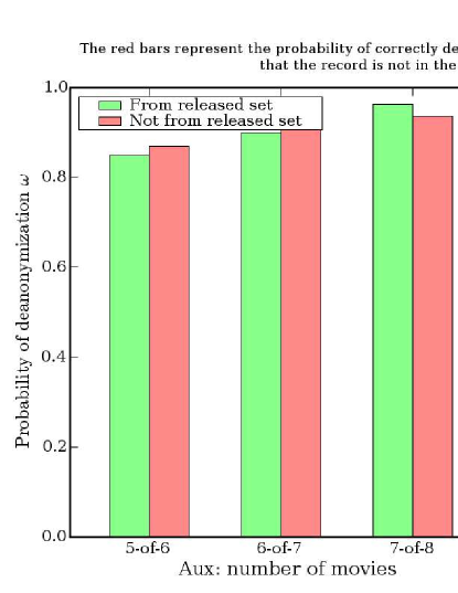
Our algorithm is specifically designed to detect when the record corresponding to aux is not in the sample. To verify this, we ran the following experiment. First, we gave aux from a random record to the algorithm and ran it on the dataset. Then we removed this record from the dataset and re-ran the algorithm. In the former case, we expect the algorithm to find the record; in the latter, to declare that the record is not in the dataset. As shown in Figure 2, the algorithm succeeds with high probability in both cases.

It is possible, although extremely unlikely, that the original Netflix dataset is not as sparse as the published sample, i.e., it contains clusters of records which are close to each other, but only one representative of each cluster has been released in the Prize dataset. A dataset with such a structure would be exceptionally unusual and theoretically problematic (see Theorem 4).

Finally, our de-anonymization algorithm is still useful even if the amount of auxiliary information available to the adversary is less than shown in Figure 2. While the absence of false positives cannot be guaranteed a priori in this case, there is a lot of additional information in the dataset that can be used to eliminate false positives. For example, consider the start date and the total number of movies in a record. If these are part of the auxiliary information (e.g., the adversary knows approximately when his target first joined Netflix), they can be used to eliminate candidate records.

Figure 1: De-anonymization: adversary knows exact ratings and approximate dates.

Figure 2: Same parameters as Figure 2, but the adversary is also required to detect when the target record is not in the sample.

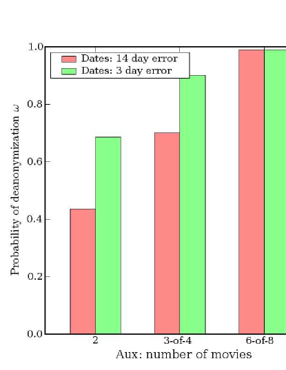
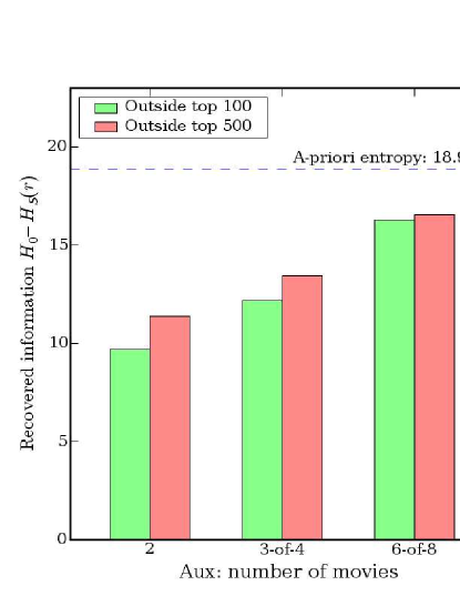
Results of de-anonymization. Very little auxiliary information is needed for de-anonymize an average subscriber record from the Netflix Prize dataset. With 8 movie ratings (of which 2 may be completely wrong) and dates that may have a 14-day error, 99% of records be uniquely identified in the dataset. For 68%, two ratings and dates (with a 3-day error) are sufficient (Figure 2). Even for the other 32%, the number of possible candidates is brought down dramatically. In terms of entropy, the additional information required for complete de-anonymization is only around 3 bits in the latter case (with no auxiliary information, this number is 19 bits). When the adversary knows 6 movies correctly and 2 incorrectly, the extra information he needs for complete de-anonymization is a fraction of a bit (Figure 4).

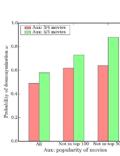
Even without any dates, a substantial privacy breach occurs, especially when the auxiliary information consists of movies that are not blockbusters (Figure 4). Two movies are no longer sufficient, but 84% of subscribers can be uniquely identified if the adversary knows 6 out of 8 moves outside the top 500 (as shown in appendix D, this is not a significant limitation).

Figure 3: Entropic de-anonymization: same parameters as in Figure 2.

Figure 4: Adversary knows exact ratings but does not know dates at all.

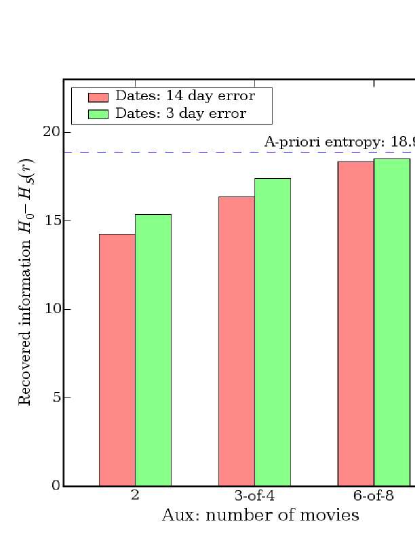
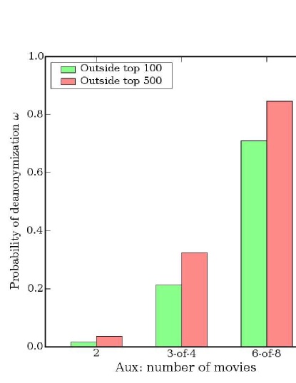
Figure 6 shows that even when the adversary’s probability to correctly determine the attributes of the target record is low, he gains a tremendous amount of information about the target record. Even in the most pessimistic scenario, the additional information he would need to complete the de-anonymization has been reduced to less than half of its original value.

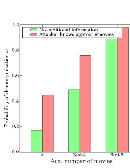
Figure 6 shows why even partial de-anonymization can be very dangerous. There are many things the adversary might know about his target that are not captured by our formal model, such as the approximate number of movies rated, the date when they joined Netflix and so on. Once a candidate set of records is available, further automated analysis or human inspection might be sufficient to complete the de-anonymization. Figure 6 shows that in some cases, knowing the number of movies the target has rated (even with a 50% error!) can more than double the probability of complete de-anonymization.

Figure 5: Entropic de-anonymization: same parameters as in Figure 4.

Figure 6: Effect of knowing approximate number of movies rated by victim ($\pm 50\%$.) Adversary knows approximate ratings($\pm 1$) and dates (14-day error).

Obtaining the auxiliary information and IMDb cross-correlation. Given how little auxiliary information is needed to de-anonymize the average subscriber record from the Netflix Prize dataset, a determined adversary should not find it difficult to obtain such information, especially since it need not be precise. A water-cooler conversation with an office colleague about her cinematographic likes and dislikes may yield enough information, especially if at least a few of the movies mentioned are outside the top 100 most rated Netflix movies. This information can also be gleaned from personal blogs, Google searches, and so on.

One possible source of users’ movie ratings is the Internet Movie Database (IMDb) [14]. We expect that for Netflix subscribers who use IMDb, there is a strong correlation between their private Netflix ratings and their public IMDb ratings. Note that our attack does not require that all movies rated by the subscriber in the Netflix system be also rated in IMDb, or vice versa. In many cases, even a handful of movies that are rated by the subscriber in both services would be sufficient to identify his or her record in the Netflix Prize dataset, if present among the released records, with enough statistical confidence to rule out the possibility of a false match except for a negligible probability.

Due to the restrictions on crawling IMDb imposed by IMDb’s terms of service (of course, a real adversary may not comply with these restrictions), we worked with a very small sample of a few dozen IMDb users. Results presented in this section should thus be viewed as a proof of concept. They do not imply anything about the percentage of IMDb users who can be identified in the Netflix Prize dataset.

The auxiliary information obtained from IMDb is quite noisy. First, a significant fraction of the movies rated on IMDb are not in Netflix, and vice versa, e.g., movies that have not been released in the US. Second, some of the ratings on IMDb are missing (i.e., the user entered only a comment, not a numerical rating). Such data are still useful for de-anonymization because an average user has rated only a tiny fraction of all movies, so the mere fact that a person has watched a given movie tremendously reduces the number of anonymous Netflix records that could possibly belong to that user. Finally, IMDb users among Netflix subscribers fall into a continuum of categories with respect to rating dates, separated by two extremes: some meticulously rate movies on both IMDb and Netflix at the same time, and others rate them whenever they have free time (which means the dates may not be correlated at all). Somewhat offsetting these disadvantages is the fact that we can use all of the user’s ratings publicly available on IMDb.

Because we have no “oracle” to tell us whether the record our algorithm has found in the Netflix Prize dataset based on the ratings of some IMDb user indeed belongs to that user, we need to guarantee a very low false positive rate. Given our small sample of IMDb users (recall that it was deliberately kept small to comply with IMDb’s terms of service), our algorithm identified the records of two users the Netflix Prize dataset with eccentricities of around 28 and 15, respectively. This is an exceptionally strong match. The records in questions are 28 standard deviations (respectively, 15 standard deviations) away from the second-best candidate. Interestingly, the first user was de-anonymized mainly from the ratings and the second mainly from the dates. Also, for nearly all the other IMDb users we tested, the eccentricity was no more than 2.

Let us summarize what our algorithm achieves. Given a user’s public IMDb ratings, which the user posted voluntarily to selectively reveal some of his (or her; but we’ll use the male pronoun without loss of generality) movie likes and dislikes, we discover all the ratings that he entered privately into the Netflix system, presumably expecting that they will remain private. A natural question to ask is why would someone who rates movies on IMDb—often under his or her real name—care about privacy of his movie ratings? Consider the information that we have been able to deduce by locating one of these users’ entire movie viewing history in the Netflix dataset and that cannot be deduced from his public IMDb ratings.

First, we can immediately find his political orientation based on his strong opinions about “Power and Terror: Noam Chomsky in Our Times” and “Fahrenheit 9/11.” Strong guesses about his religious views can be made based on his ratings on “Jesus of Nazareth” and “The Gospel of John”. He did not like “Super Size Me” at all; perhaps this implies something about his physical size? Both items that we found with predominantly gay themes, “Bent” and “Queer as folk” were rated one star out of five. He is a cultish follower of “Mystery Science Theater 3000”. This is far from all we found about this one person, but having made our point, we will spare the reader further lurid details.

6 Conclusions

We have presented a de-anonymization methodology for multi-dimensional micro-data, and demonstrated its practical applicability by showing how to de-anonymize movie viewing records released in the Netflix Prize dataset. Our de-anonymization algorithm works under very general assumptions about the distribution from which the data are drawn, and is robust to perturbation and sanitization. Therefore, we expect that it can be successfully used against any large dataset containing anonymous multi-dimensional records such as individual transactions, preferences, and so on.

An interesting topic for future research is extracting social relationships, networks and clusters from the anonymous records. This knowledge can be a source of information for further de-anonymization [13]. In the case of the Netflix Prize dataset, de-anonymization of individual records may also have interesting implications for winning the Netflix Prize. We discuss this briefly in appendix B.

Appendix A Glossary of terms

Symbol	Meaning
$D$	Database
${\hat{D}}$	Released sample
$N$	Number of rows
$M$	Number of columns
$m$	Size of aux
$X$	Domain of attributes
$\perp$	Null attribute
$\textsf{supp}(.)$	Set of non-null attributes in a row/column
Sim	Similarity measure
Aux	Auxiliary information sampler
aux	Auxiliary information
Score	Scoring function
$\epsilon$	Sparsity threshold
$\delta$	Sparsity probability
$\theta$	Closeness of de-anonymized record
$\omega$	Probability of success of de-anonymization
$r,r^{\prime}$	Record
$\Pi$	P.d.f over records
$H_{S}$	Shannon entropy
$H$	De-anonymization entropy
$\phi$	Eccentricity

Appendix B Implications for the Netflix Prize

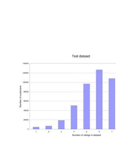
De-anonymization of Netflix subscribers may enable one to learn the true ratings for some entries in the Netflix Prize test dataset (these ratings have been kept secret by Netflix). The test dataset has been chosen in such a way that the contribution of any given subscriber is no more than 9 entries (see Figure 7). Therefore, it is not possible to find a small fraction of subscribers whose ratings will reveal a large fraction of the test dataset.

Access to true ratings on the test dataset does not translate to an immediate strategy for claiming the Netflix Prize. The rules require that the algorithm be submitted for perusal. In spite of this, having the test data (or the data closely correlated with the test data) enables the contestant to train on the test data in order to “overfit” the model. This is why Netflix kept the ratings on the test data secret.

Figure 7: Test dataset for the Netflix Prize.

How many Netflix subscribers would need to be de-anonymized before there is a significant impact on the performance of a recommendation algorithm that uses this information? The root mean squared errors (RMSE) of the current top performers (as of November 9, 2007) are about $0.87$. If a subscriber’s “true” ratings are available, the error for that subscriber drops to zero. Thus, if the learner has access to $\frac{1}{0.87}=1.14\%$ of de-anonymized records, then the RMSE score improves by 1% (assuming that the contribution of each subscriber is the same and RMSE behaves roughly linearly). This is roughly equal to the difference the current 1st and 20th contestants on the Netflix Prize leader board.

How easy is it to de-anonymize 1% of the subscribers? The potential sources of large-scale true rating data are the publicly available ratings on the site itself, public ratings on other movie websites such as IMDb, and the subscribers themselves. Netflix appears to have taken the elementary precaution of removing from the dataset the ratings of the subscribers that are publicly available on the Netflix website. While our experiments in section 6 show that successful cross-correlation of IMDb and Netflix records is possible, there are some hurdles to overcome: it is not clear what fraction of users with a significant body of movie ratings on IMDb are also Netflix subscribers, nor is it known how ratings and dates on IMDb correlate with those on Netflix for the average user (although we expect a strong correlation).

Collecting data from the subscribers themselves appears to be the most promising direction. Many Netflix subscribers do not regard their ratings as private data and are eager to share them, to the extent that there even exists a browser plugin that automates this process, although we have not found any public rating lists generated this way. If the here-are-all-my-Netflix-ratings “meme” propagates through the “blogosphere,” it could easily result in a publicly available dataset of sufficiently large size. It is also easy for a malicious person to bribe subscribers (say, “upload your Netflix ratings to gain access to the protected areas of this site”). Also, many subscribers have “friends” on Netflix, and subscribers’ ratings are accessible to their friends.

We emphasize that even though many Netflix subscribers do not regard their movie viewing histories as sensitive, this does not mean that privacy of Netflix records is moot. In section 6, we extracted from the Netflix Prize dataset non-public information about some subscribers that should be considered sensitive by any reasonable definition.

Appendix C On perturbation of the Netflix Prize dataset

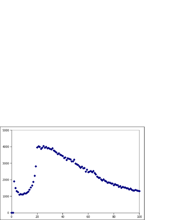
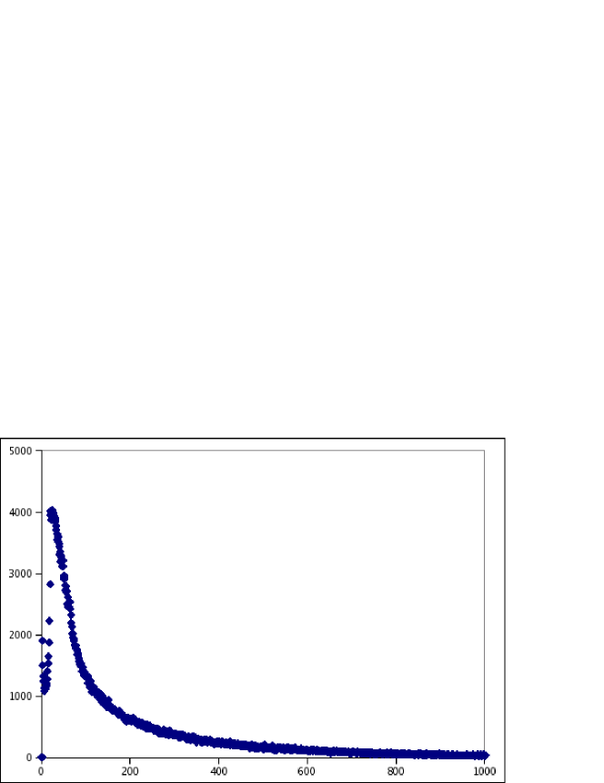
Figs. 9 and 9 plot the number of ratings $X$ against the number of subscribers in the released dataset who have at least $X$ ratings. The tail is surprisingly thick: thousands of subscribers have rated more than a thousand movies. Netflix claims that the subscribers in the released dataset have been “randomly chosen.” Whatever the selection algorithm was, it was not uniformly random. Common sense suggests that with uniform subscriber selection, the curve would be monotonically decreasing (as most people rate very few movies or none at all), and that there would be no sharp discontinuities.

It is not clear how the data was sampled. Our conjecture is that some fraction of the subscribers with more than 20 ratings were sampled, and the points on the graph to the left of $X=20$ are the result of some movies being deleted after the subscribers were sampled.

We requested the rating history as presented on the Netflix website from some of our acquaintances, and based on this data (which is effectively drawn from Netflix’s original, non-anonymous dataset, since we know the names associated with these records), located two of them in the Netflix Prize dataset. Netflix’s claim that the data were perturbed [20] does not appear to be borne out. One of the subscribers had 1 of 306 ratings altered, and the other had 5 of 229 altered. (These are upper bounds, because they include the possibility that the subscribers changed the ratings after the 2005 snapshot that was released was taken.) In any case, the level of noise is far too small to affect our de-anonymization algorithms, which have been specifically designed to withstand this kind of imprecision. We have no way of determining how many dates were altered and how many ratings were deleted, but we conjecture that very little perturbation has been applied.

It is important that the Netflix Prize dataset has been released to support development of better recommendation algorithms. A significant perturbation of individual attributes would have affected cross-attribute correlations and significantly decreased the dataset’s utility for creating new recommendation algorithms, defeating the entire purpose of the Netflix Prize competition.

Finally, we observe that the Netflix Prize dataset clearly has not been $k$-anonymized for any value of $k>1$.

Figure 8: For each $k\leq 100$, the number of subscribers with $k$ ratings in the released dataset.

Figure 9: For each $k\leq 1000$, the number of subscribers with $k$ ratings in the released dataset.

Appendix D Marginals

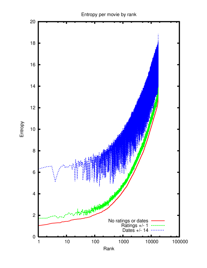
In Figure 11, we demonstrate how much information the adversary gains about his target from the knowledge of one of the movies watched by the target, as a function of the rank of the movie. This helps visualize how the adversary’s success varies depending on whether the movies are randomly picked, or if they are constrained to be outside the top 100 or top 500. Of course, since there are correlations between the lists of subscribers who watched different movies, we cannot simply multiply the information gain per movie by the number of movies. Therefore, this graph cannot be used to infer how many attributes must be part of the auxiliary information before the adversary can successfuly de-anonymize.

Figure 10: Entropy of movie by rank

Figure 11: Effect of knowing less popular movies rated by victim. Adversary knows approximate ratings ($\pm 1$) and dates (14-day error).

Finally, we show the relationship between subscribers and the ranks of the movies they rated.

	Percentage of subscribers who rated …
	At least 1 movie	At least $5$	At least $10$
Not in 100 most rated	100%	97%	93%
Not in 500 most rated	99%	90%	80%
Not in 1000 most rated	97%	83%	70%

Figure 11 explores in greater detail the effect of the popularity of movies known to the adversary. The effect is not negligible, but not dramatic either.

Appendix E Sparsity

The chart demonstrates that most Netflix subscribers do not have even a single subscriber with a high similarity score ($>0.5$), even if we consider only the respective sets of movies rated without taking into account numerical ratings or dates on these movies.

Figure 12: X-axis ($x$) is the similarity to nearest neighbor: i.e, the subscriber with the highest similarity score. Y-axis is the fraction of subscribers whose nearest neighbor similarity is at least $x$.

References

- [1] N. Adam and J. Worthmann. Security-control methods for statistical databases: A comparative study. ACM Computing Surveys, 21(4):515–556, 1989.
- [2] C. Aggarwal. On k-anonymity and the curse of dimensionality. In Proc. 31st International Conference on Very Large Data Bases (VLDB), pages 901–909. ACM, 2005.
- [3] R. Agrawal and R. Srikant. Privacy-preserving data mining. In Proc. 2000 ACM SIGMOD International Conference on Management of Data, pages 439–450. ACM, 2000.
- [4] C. Anderson. The Long Tail: Why the Future of Business Is Selling Less of More. Hyperion, 2006.
- [5] A. Blum, C. Dwork, F. McSherry, and K. Nissim. Practical privacy: The SuLQ framework. In Proc. 24th ACM SIGACT-SIGMOD-SIGART Symposium on Principles of Database Systems (PODS), pages 128–138. ACM, 2005.
- [6] E. Brynjolfsson, Y. Hu, and M. Smith. Consumer surplus in the digital economy. Management Science, 49(11), 2003.
- [7] S. Chawla, C. Dwork, F. McSherry, A. Smith, and H. Wee. Towards privacy in public databases. In Proc. 2nd Theory of Cryptography Conference (TCC), volume 3378 of LNCS, pages 363–385. Springer, 2005.
- [8] V. Ciriani, S. De Capitani di Vimercati, S. Foresti, and P. Samarati. k-anonymity. Secure Data Management in Decentralized Systems, 2007.
- [9] C. Díaz, S. Seys, J. Claessens, and B. Preneel. Towards measuring anonymity. In Proc. 2nd International Workshop on Privacy-Enhancing Technologies, volume 2482 of LNCS, pages 54–68, 2002.
- [10] D. Frankowski, D. Cosley, S. Sen, L. Terveen, and J. Riedl. You are what you say: privacy risks of public mentions. In Proc. 29th Annual ACM SIGIR Conference on Research and Development in Information Retrieval, pages 565–572. ACM, 2006.
- [11] K. Hafner. And if you liked the movie, a Netflix contest may reward you handsomely. New York Times, Oct 2 2006.
- [12] S. Hansell. AOL removes search data on vast group of web users. New York Times, Aug 8 2006.
- [13] B. Hayes. Connecting the dots: Can the tools of graph theory and social-network studies unravel the next big plot? American Scientist, September–October 2006. http://www.americanscientist.org/template/AssetDetail/assetid/53062.
- [14] IMDb. The Internet Movie Database. http://www.imdb.com/, 2007.
- [15] J. L. W. V. Jensen. Sur les fonctions convexes et les inégalités entre les valeurs moyennes. Acta Mathematica, 30(1):175–193, 1906.
- [16] J. Leskovec, L. Adamic, and B. Huberman. The dynamics of viral marketing. In Proc. 7th ACM Conference on Electronic Commerce, pages 228–237. ACM, 2006.
- [17] A. Machanavajjhala, J. Gehrke, D. Kifer, and M. Venkitasubramaniam. l-diversity: Privacy beyond k-anonymity. In Proc. 22nd International Conference on Data Engineering (ICDE). IEEE Computer Society, 2006.
- [18] A. Machanavajjhala, D. Martin, D. Kifer, J. Gehrke, and J. Halpern. Worst case background knowledge. In Proc. 23rd International Conference on Data Engineering (ICDE). IEEE Computer Society, 2007.
- [19] B. Malin and L. Sweeney. How (not) to protect genomic data privacy in a distributed network: using trail re-identification to evaluate and design anonymity protection systems. J. of Biomedical Informatics, 37(3):179–192, 2004.
- [20] Netflix. Netflix Prize: FAQ. http://www.netflixprize.com/faq, Downloaded on Oct 17 2006.
- [21] A. Serjantov and G. Danezis. Towards an information theoretic metric for anonymity. In Proc. 2nd International Workshop on Privacy Enhancing Technologies (PET), volume 2482 of LNCS, pages 41–53. Springer, 2003.
- [22] L. Sweeney. Weaving technology and policy together to maintain confidentiality. J. of Law, Medicine and Ethics, 25(2–3):98–110, 1997.
- [23] L. Sweeney. Achieving k-anonymity privacy protection using generalization and suppression. International J. of Uncertainty, Fuzziness and Knowledge-based Systems, 10(5):571–588, 2002.
- [24] L. Sweeney. k-anonymity: A model for protecting privacy. International J. of Uncertainty, Fuzziness and Knowledge-based Systems, 10(5):557–570, 2002.
- [25] J. Thornton. Collaborative filtering research papers. http://jamesthornton.com/cf/, 2006.
- [26] J. Traub, Y. Yemini, and H. Wozniakowski. The statistical security of a statistical database. ACM Transactions on Database Systems, 9(4):672–679, 1984.
- [27] L. Zhang, S. Jajodia, and A. Brodsky. Information disclosure under realistic assumptions: Privacy versus optimality. In Proc. 14th ACM Conference on Computer and Communications Security (CCS). ACM, 2007.