MIMO BROADCAST CHANNELS WITH BLOCK DIAGONALIZATION AND FINITE RATE FEEDBACK

Abstract

Block diagonalization is a linear precoding technique for the multiple antenna broadcast (downlink) channel that involves transmission of multiple data streams to each receiver such that no multi-user interference is experienced at any of the receivers. This low-complexity scheme operates only a few dB away from capacity but does require very accurate channel knowledge at the transmitter, which can be very difficult to obtain in fading scenarios. We consider a limited feedback system where each receiver knows its channel perfectly, but the transmitter is only provided with a finite number of channel feedback bits from each receiver. Using a random vector quantization argument, we quantify the throughput loss due to imperfect channel knowledge as a function of the feedback level. The quality of channel knowledge must improve proportional to the SNR in order to prevent interference-limitations, and we show that scaling the number of feedback bits linearly with the system SNR is sufficient to maintain a bounded rate loss. Finally, we investigate a simple scalar quantization scheme that is seen to achieve the same scaling behavior as vector quantization.

Index Terms—  MIMO systems, Broadcast channels, Quantization, Finite Rate Feedback, Multiplexing Gain

1 Introduction

In multiple antenna broadcast (downlink) channels, transmit antenna arrays can be used to simultaneously transmit data streams to receivers and thereby significantly increase throughput. Dirty paper coding (DPC) is capacity achieving for the MIMO broadcast channel [1], but this technique has a very high level of complexity. Zero Forcing (ZF) and Block Diagonalization (BD) [2] [3] are alternative low-complexity transmission techniques. Although not optimal, these linear precoding techniques utilize all available spatial degrees of freedom and perform measurably close to DPC in many scenarios [4].

If the transmitter is equipped with $M$ antennas and there are at least $M$ aggregate receive antennas, zero-forcing involves transmission of $M$ spatial beams such that independent, de-coupled data channels are created from the transmit antenna array to $M$ receive antennas distributed amongst a number of receivers. Block diagonalization similarly involves transmission of $M$ spatial beams, but the beams are selected such that the signals received at different receivers, but not necessarily at the different antenna elements of a particular receiver, are de-coupled. For example, if there are $M/2$ receivers with two antennas each, then two beams are aimed at each of the receivers. If ZF is used, an independent and de-coupled data stream is received on each of the $M$ antennas. If BD is used, the streams for different receivers do not interfere, but the two streams intended for a single receiver are generally not aligned with its two antennas and thus post-multiplication by a rotation matrix (to align the streams) is generally required before decoding.

In order to correctly aim the transmit beams, both schemes require perfect Channel State Information at the Transmitter (CSIT). Imperfect CSIT leads to incorrect beam selection and therefore multiuser interference, which ultimately leads to a throughput loss. Unlike point to point MIMO systems where imperfect CSIT causes only an SNR offset in the capacity vs. SNR curve, the level of CSIT affects the slope of the curve and hence the multiplexing gain in broadcast MIMO systems. We consider the case when the CSI is known perfectly at the receiver and is communicated to the transmitter through a finite rate feedback channel and quantify the maximum rate loss due to finite rate feedback with BD. MISO systems and ZF with finite rate feedback are analyzed in [5]. Similar to the results in [5], we show that scaling the number of feedback bits approximately linearly with the system SNR is sufficient to maintain the slope of the capacity vs. SNR curve and hence a constant gap from the capacity of BD with perfect CSIT. The scaling factor for BD offers an advantage over ZF in terms of the number of bits required to achieve the same sum capacity. Finally, we investigate a simple scalar quantization scheme and see that this low complexity scheme requires the same feedback scaling.

2 System Model

We consider a single transmitter and $K$ user MIMO system where each user has $N$ antennas and the transmitter has $M$ antennas. The broadcast channel is described as:

$${\mathbf{y}}_{i}={\mathbf{H}}_{i}^{H}{\mathbf{x}}+{\bf n}_{i},\quad i=1,\dots,K$$ (1)

where ${\mathbf{H}}_{i}\in\mathbb{C}^{M\times N}$ is the channel matrix from the transmitter to the $i^{\text{th}}$ user ($1\leq i\leq K$) and the vector ${\mathbf{x}}\in\mathbb{C}^{M\times 1}$ is the transmitted signal. ${\bf n}_{i}\in\mathbb{C}^{N\times 1}$ are independent complex Gaussian noise vectors of unit variance and ${\mathbf{y}}_{i}\in\mathbb{C}^{N\times 1}$ is the received signal vector at the $i^{\text{th}}$ user. We assume a transmit power constraint so that $E[||{\mathbf{x}}||^{2}]\leq P$ $(P>0)$. We also assume that $K>1$ and $K=\frac{M}{N}$, which implies that the aggregate number of receive antennas equals the number of transmit antennas; as a result it is not necessary to select a subset of receivers for transmission.

The entries of ${\mathbf{H}}_{i}$ are assumed to be i.i.d. unit variance complex Gaussian random variables, and the channel is assumed to be block fading with independent fading from block to block. Each of the receivers is assumed to have perfect and instantaneous knowledge of their own channel matrix. The channel matrix is quantized at each receiver and fed back to the transmitter (which has no other knowledge of the instantaneous CSI) over a zero delay, error free, finite rate channel. In order to perform BD, it is only necessary to know the spatial direction of each receiver’s channel, i.e., the subspace spanned by ${\mathbf{H}}_{i}$, and thus the feedback only conveys this information.

2.1 Finite Rate Feedback Model

The quantization codebook used at each receiver is fixed beforehand and is known to the transmitter and each receiver. A quantization codebook ${\mathcal{C}}$ consists of $2^{B}$ matrices in $\mathbb{C}^{M\times N}$ i.e. $({\mathbf{W}}_{1},$ $\dots,{\mathbf{W}}_{2^{B}})$, where $B$ is the feedback bits per user. The quantization of a channel matrix ${\mathbf{H}}_{i}$, say $\hat{\mathbf{H}}_{i}$, is chosen from the codebook ${\mathcal{C}}$ according to:

$$\hat{\mathbf{H}}_{i}=\mathop{\arg\min}\limits_{{\mathbf{W}}\ \in\ {\mathcal{C}}}\ d^{2}\left({\mathbf{H}}_{i},{\mathbf{W}}\right)$$ (2)

where $d\left({\mathbf{H}}_{i},{\mathbf{W}}\right)$ is the distance metric. Here, we consider the chordal distance [6]:

$$d\left({\mathbf{H}}_{i},{\mathbf{W}}\right)=\sqrt{\sum\limits_{i=1}^{N}\sin^{2}\theta_{i}}$$ (3)

where the $\theta_{i}$’s are the principal angles between the two subspaces spanned by the columns of the matrices. As the principal angles depend only on the subspaces spanned by the columns of the matrices, it can be assumed that the elements of ${\mathcal{C}}$ unitary matrices. No channel magnitude information is fed back to the transmitter.

2.2 Random Quantization Codebooks

Since the design of optimal quantization codebooks for the given distance metric is a very difficult problem, we instead study performance averaged over random quantization codebooks. The Grassmannian manifold is the set of all $N$ dimensional subspaces in an $M$ dimensional Euclidean space, and is denoted by $\mathbb{G_{\text{M,N}}(\mathbb{C})}$. Each of the $2^{B}$ matrices making up the random quantization codebook is chosen independently and uniformly distributed over $\mathbb{G_{\text{M,N}}(\mathbb{C})}$, and each matrix can be assumed to be unitary (points in $\mathbb{G_{\text{M,N}}(\mathbb{C})}$ are equivalence classes of orthonormal matrices in $\mathbb{C}^{M\times N}$). We analyze the performance averaged over all possible random codebooks. The distortion or error associated with a given codebook ${\mathcal{C}}$ for the quantization of ${\mathbf{H}}\in\mathbb{C}^{M\times N}$ is defined as:

$$D=E\left[d^{2}({\mathbf{H}},\hat{\mathbf{H}})\right]=E\left[\mathop{\min\limits_{{\mathbf{W}}\in{\mathcal{C}}}}\ d^{2}({\mathbf{H}},{\mathbf{W}})\right]$$ (4)

where $\hat{\mathbf{H}}$ is the quantization of ${\mathbf{H}}$. It is shown in [7] $D$ satisfies:

$$D\ \leq\ \frac{\Gamma(\frac{1}{T})}{T}(C_{MN})^{-\frac{1}{T}}2^{-\frac{B}{T}}+N\exp\left[-(2^{B}C_{MN})^{1-a}\right]=\overline{D}$$ (5)

for a codebook of size $2^{B}$, where $T=N(M-N)$ and $a\in(0,1)$ is a real number between $0$ and $1$ chosen such that $\left(C_{MN}2^{B}\right)^{-\frac{a}{T}}\leq 1$. $C_{MN}$ is given by $\frac{1}{T!}\ \prod\limits_{i=1}^{N}\ \frac{(M-i)!}{(N-i)!}$. The second (exponential) term in (5) for the expression of $D$ can be neglected for large $B$.

2.3 Block Diagonalization

The Block Diagonalization strategy when perfect CSI is available at the transmitter involves precoding the signals to be transmitted in order to suppress interference at each user due to all other users (but not due to different antennas for the same user). If ${\mathbf{s}}_{i}\in\mathbb{C}^{N\times 1}$ contains the $N$ complex symbols intended for the $i^{\text{th}}$ ($1\leq i\leq K$) user and ${\mathbf{V}}_{i}\in\mathbb{C}^{M\times N}$ is the precoding matrix, then the transmitted vector is given by:

$${\mathbf{x}}=\sqrt{\frac{P}{K}}\sum\limits_{i=1}^{K}\ {\mathbf{V}}_{i}{\mathbf{s}}_{i}$$ (6)

and the received signal at the $i^{\text{th}}$ user is given by:

$${\mathbf{y}}_{i}=\sqrt{\frac{P}{K}}{\mathbf{H}}_{i}^{H}{\mathbf{V}}_{i}{\mathbf{s}}_{i}+\sqrt{\frac{P}{K}}\sum\limits_{j=1,j\neq i}^{K}\ {\mathbf{H}}_{i}^{H}{\mathbf{V}}_{j}{\mathbf{s}}_{j}+{\bf n}_{i}$$ (7)

It is assumed that a uniform power allocation strategy among users is employed (due to absence of channel magnitude information at the transmitter). Furthermore, in order to maintain the power constraint it is assumed that ${\mathbf{V}}_{i}^{H}{\mathbf{V}}_{i}={\bf I_{N}}$ and $E[||{\mathbf{s}}_{i}||^{2}]\leq 1$.

Following the BD strategy, each ${\mathbf{V}}_{i}$ is chosen such that ${\mathbf{H}}_{j}^{H}{\mathbf{V}}_{i}$ is ${\bf 0},\ \forall i\neq j$. This amounts to determining an orthonormal basis for the null space of the matrix formed by stacking all ${\mathbf{H}}_{j},j\neq i$ matrices together. This reduces the interference terms in equation (7) to zero at each user. This is different from Zero Forcing where each complex symbol to be transmitted to the $m^{\text{th}}$ antenna (among the $N$ antennas) of the $i^{\text{th}}$ user is precoded by a vector that is orthogonal to all the columns of ${\mathbf{H}}_{j\neq i}$ as well as orthogonal to all but the $m^{\text{th}}$ column of ${\mathbf{H}}_{i}$.

However, perfect knowledge of the ${\mathbf{H}}_{i}$’s at the transmitter is required for zero interference. When finite rate feedback is employed, each ${\mathbf{V}}_{i}$ is chosen such that $\hat{\mathbf{H}}_{j}^{H}{\mathbf{V}}_{i}={\bf 0}\ \forall i\neq j$ which is $\neq{\mathbf{H}}_{j}^{H}{\mathbf{V}}_{i}$ in general, and leads to a loss in throughput.

3 Throughput Analysis

3.1 Fixed Feedback Quality

In the case of perfect CSIT and BD, the transmitter has the ability to suppress all interference terms giving a per user ergodic capacity of:

$$R_{BD}(P)=E_{\mathbf{H}}\left[\ \log_{2}\left|{\bf I_{N}}+\frac{P}{K}\ {\mathbf{H}}^{H}{\mathbf{V}}_{BD}{\mathbf{V}}_{BD}^{H}{\mathbf{H}}\right|\ \right]$$ (8)

where ${\mathbf{V}}_{BD}$ is the precoding matrix chosen by the BD procedure given the channels of all the users. The expectation is carried out over all channels ${\mathbf{H}}$.

For finite rate feedback of $B$ bits per user, multiuser interference cannot be perfectly canceled and leads to additional noise power. Taking this interference into account, the per user throughput is:

$$R_{FB}(P)=E_{{\mathbf{H}}_{i},{\mathcal{C}}}\left[\log_{2}\left|{\bf I_{N}}+\frac{P}{K}\sum\limits_{j=1}^{K}\ {\mathbf{H}}_{i}^{H}{\mathbf{V}}_{j}{\mathbf{V}}_{j}^{H}{\mathbf{H}}_{i}\right|\right]-$$

$$E_{{\mathbf{H}}_{i},{\mathcal{C}}}\left[\log_{2}\left|{\bf I_{N}}+\frac{P}{K}\sum\limits_{j=1,j\neq i}^{K}{\mathbf{H}}_{i}^{H}{\mathbf{V}}_{j}{\mathbf{V}}_{j}^{H}{\mathbf{H}}_{i}\right|\right]$$ (9)

where the expectation is carried out over all channels as well as random codebooks ($i$ is any user between $1$ and $K$).

Theorem 3.1.

The rate loss per user incurred due to finite rate feedback with respect to perfect CSIT using Block Diagonalization can be bounded from above by:

$$\Delta R(P) = \left[R_{BD}(P)-R_{FB}(P)\right]$$

$$\leq N\ \log_{2}(1+PD)$$

Proof.

$\Delta R(P)=\left[R_{BD}(P)-R_{FB}(P)\right]$

$$\mathop{\leq}\limits^{\text{\tiny{(a)}}} E_{\mathbf{H}}\left[\log_{2}\left|{\bf I_{N}}+\frac{P}{K}\ {\mathbf{H}}^{H}{\mathbf{V}}_{BD}{\mathbf{V}}_{BD}^{H}{\mathbf{H}}\right|\ \right]-$$

$$E_{{\mathbf{H}}_{i},{\mathcal{C}}}\left[\ \log_{2}\left|{\bf I_{N}}+\frac{P}{K}\ {\mathbf{H}}_{i}^{H}{\mathbf{V}}_{i}{\mathbf{V}}_{i}^{H}{\mathbf{H}}_{i}\right|\ \right]+$$

$$E_{{\mathbf{H}}_{i},{\mathcal{C}}}\left[\ \log_{2}\left|{\bf I_{N}}+\frac{P}{K}\sum\limits_{j=1,j\neq i}^{K}\ {\mathbf{H}}_{i}^{H}{\mathbf{V}}_{j}{\mathbf{V}}_{j}^{H}{\mathbf{H}}_{i}\right|\ \right]$$

$$\mathop{=}\limits^{\text{\tiny{(b)}}} E_{{\mathbf{H}}_{i},{\mathcal{C}}}\left[\ \log_{2}\left|{\bf I_{N}}+\frac{P}{K}\sum\limits_{j=1,j\neq i}^{K}\ {\mathbf{H}}_{i}^{H}{\mathbf{V}}_{j}{\mathbf{V}}_{j}^{H}{\mathbf{H}}_{i}\right|\ \right]$$

$$\mathop{=}\limits^{\text{\tiny{(c)}}} E_{{\mathbf{H}}_{i},{\mathcal{C}}}\left[\log_{2}\left|{\bf I_{N}}+\frac{P}{K}\tilde{{\mathbf{H}}}_{i}^{H}\left(\sum\limits_{j\neq i}{\mathbf{V}}_{j}{\mathbf{V}}_{j}^{H}\right)\tilde{{\mathbf{H}}}_{i}{\bf\Lambda}_{i}\right|\right]$$

$$\mathop{\leq}\limits^{\text{\tiny{(d)}}} \log_{2}\ \left|{\bf I_{N}}+\frac{P(K-1)}{K}E_{{\mathbf{H}},{\mathcal{C}}}\left[\tilde{{\mathbf{H}}}_{i}^{H}\left({\mathbf{V}}_{j}{\mathbf{V}}_{j}^{H}\right)\tilde{{\mathbf{H}}}_{i}\right]M\right|$$

Here, bound (a) follows by neglecting the positive semi definite interference terms. Both ${\mathbf{V}}_{BD}$ and ${\mathbf{V}}_{i}$ are uniformly distributed and independent of ${\mathbf{H}}_{i}$ which results in (b). We write ${\mathbf{H}}_{i}{\mathbf{H}}_{i}^{H}=\tilde{{\mathbf{H}}}_{i}{\bf\Lambda_{i}}\tilde{{\mathbf{H}}}_{i}^{H}$ where $\tilde{{\mathbf{H}}}_{i}$ forms an orthonormal basis for the subspace spanned be the columns of ${\mathbf{H}}_{i}$ and ${\bf\Lambda_{i}}=\text{diag}[\lambda_{1},\dots,\lambda_{N}]$ are the $N$ non-zero unordered eigen values of ${\mathbf{H}}_{i}{\mathbf{H}}_{i}^{H}$ (assuming ${\mathbf{H}}_{i}$ is of rank $N$ and diagonalizable) where $E\left[{\bf\Lambda_{i}}\right]$ is $M{\bf I}_{N}$, and (c) follows. The bound (d) follows from Jensen’s inequality due to the concavity of $\log|\cdot|$. It can also be shown that $E_{{\mathbf{H}},{\mathcal{C}}}\left[\tilde{{\mathbf{H}}}_{i}^{H}\left({\mathbf{V}}_{j}{\mathbf{V}}_{j}^{H}\right)\tilde{{\mathbf{H}}}_{i}\right]=\frac{D}{M-N}$, which provides a bound on the rate loss per user. $D$ can be upper bounded by $\overline{D}$ from (5) for large enough $B$. ∎

3.2 Increasing Feedback Quality

Theorem 3.2.

In order to maintain a rate loss $\Delta R(P)$ of no larger than $\log_{2}(b)>0$ per user, it is sufficient for the number of feedback bits per user to be scaled with SNR as:

$$B\approx \frac{N(M-N)}{3}P_{dB}-N(M-N)\log_{2}(b^{\frac{1}{N}}-1)\ +$$ (10)

$$N(M-N)\log_{2}\left[\frac{\Gamma(\frac{1}{N(M-N)})}{N(M-N)}\right]-\log_{2}(C_{MN})$$

This expression can be found by equating the upper bound on rate loss with $\log_{2}b$ and solving for $B$ as a function of $P$. Solving this numerically will yield the number of bits strictly sufficient for a maximum rate loss of $log_{2}b$. We assume that $B$ is large enough to neglect the exponential term in the expression for $\overline{D}$ from (5) which yields the above approximation. The total contribution of the term containing the logarithm of the gamma function is less than a bit and it can usually be neglected. To maintain a system throughput loss of $M$ bps/Hz, which corresponds to an SNR gap of no more than $3$ dB with respect to BD with perfect CSIT, it is sufficient to scale the bits as:

$$B\approx\frac{N(M-N)}{3}P_{dB}-\log_{2}(C_{MN})$$ (11)

The factor of $N(M-N)$ suggests that the number of feedback bits per antenna reduce with increasing $N$. The number of bits can grow very large for MIMO broadcast systems, and simulation becomes a computationally complex task. However, utilizing the statistics of random codebooks, systems with a small number of antennas can be simulated in a reasonable amount of time. We present simulation results for $M=8$ and $N=2$ in Figure 1(a) while scaling the bits as per (11). As Theorem 3.2 only provides the sufficient number of bits, this is a conservative strategy and the actual SNR gap is found to be $2.3$dB instead of $3$dB. The simulations also suggest that keeping the number of bits fixed will result in rate loss which increases with SNR. Similar results are presented in Figure 1(b) for an $N=3$ system.

4 Zero forcing vs. Block diagonalization

Zero forcing is an even simpler strategy than BD, and it is important to compare the performance of these two schemes under the presence of limited feedback. Zero forcing for a MIMO broadcast system with $K$ users and $N$ antennas per user is equivalent to a $KN=M$ user system with a single antenna per user. The feedback scaling law for such a system is derived in [5] to be:

$$B_{ZF}\approx\frac{(M-1)}{3}P_{dB}$$ (12)

to maintain an SNR gap of no more than $3$ dB with respect to ZF under perfect CSIT conditions. In general, BD achieves a higher sum rate than ZF with perfect CSIT where the rate gap is $Klog_{2}(e)$ $\sum_{j=1}^{N}\frac{N-j}{j}$ [8] at high SNR. In order to compare the number of bits required for BD and ZF under imperfect CSIT and finite rate feedback, it is necessary to fix a common target rate. The bits required per user for ZF must also be multiplied by $N$ for fair comparison. By setting $b=2^{R_{g}+R}$ in (10) where $R_{g}$ is the per user rate gap between BD and ZF with perfect CSIT and $R$ the target per user rate loss for the ZF system, we can compare the sufficient number of bits required to achieve the same sum rate for both strategies. For example, $R=1$ for a $3$ dB target and this suggests a bit savings of 20% for an $M=6,N=2$ system, and 25% for an $M=9,N=3$ system with BD. The scaling law in Theorem 3.2 is however highly conservative for large $b$, and though it is possible to see that BD has a clear advantage in terms of the sufficient number of bits required, it is somewhat underestimated. If a ZF system is scaled to maintain a $3$dB SNR gap relative to perfect CSIT and the number of feedback bits for BD is numerically determined to achieve the same sum rate, bit savings are about 40-50% for an $M=6,N=2$ system.

5 Quantizing the Channel

The scaling law in Section 3.2 was derived considering random codebooks, which are impractical for real world applications. Although vector quantization codebooks can be designed for more practical systems it is likely to require very high complexity due to the large number of bits at each mobile. It is thus worthwhile to investigate low complexity scalar quantization schemes. We believe that simple scalar quantization methods are capable of achieving the same bit scaling rate as random codes, though they will incur a constant rate loss.

The scalar quantization scheme is first presented for MISO systems (based on the idea in [9]). A complex channel vector ${\mathbf{H}}_{i}=[H_{1},\dots,H_{M}]^{H}\in\mathbb{C}^{M\times 1}$ is first divided by one of its elements, say $H_{1}$, to yield $M-1$ complex elements. The phase of each of these elements is quantized separately and uniformly in the interval $[-\pi,\pi]$. The inverse tangents of the magnitudes, for example $\tan^{-1}\left(\frac{|H_{2}|}{|H_{1}|}\right)$, are quantized uniformly in the interval $[0,\frac{\pi}{2}]$. Nonuniform quantization based on the distribution of these random variables is also possible, but (sub-optimal) uniform quantization appears to be sufficient for the number of feedback bits to scale linearly with SNR with the same slope as with random codebooks. The total number of bits available to a user is assumed to be distributed equally among the phases and magnitudes of the $M-1$ elements as far as possible, and the remaining bits are randomly assigned.

For MIMO systems, this is generalized to quantizing the magnitude and phase (in the same manner) of the lower $(M-N)\times N$ entries of the matrix ${\mathbf{H}}_{i}([{\bf I}_{1}\ |\ {\bf Z}_{1}]{\mathbf{H}}_{i})^{-1}$. ${\bf I}_{1}$ is the $N\times\frac{M}{2}$ identity matrix and ${\bf Z}_{1}$ the $N\times\frac{M}{2}$ zero matrix.

Although we do not offer an analytical proof that this scheme achieves the same bit scaling rate as random codebook quantization, we present simulation results that certainly suggest this. The bits for scalar quantization are scaled according to Equation (12) for an $M=6,N=1$ MISO system (Figure 2). This maintains a constant gap with the perfect CSIT curve, although there is a $2.7$ dB SNR loss with respect to random codebook quantization. More sophisticated scalar quantization methods may be able to reduce this gap as well, which indicates that simple scalar quantization schemes could perform quite well. Similar results for MIMO systems are presented in Figures 1(a) and 1(b) with $4$ and $2$ users respectively.

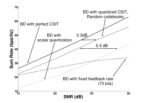
(a) MIMO Broadcast Channel with M = 8, N = 2, K = 4

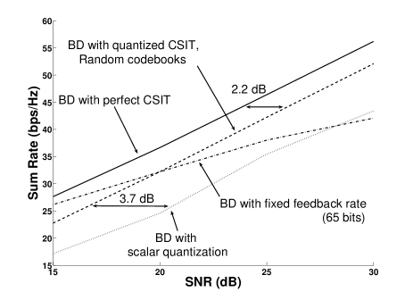
(b) MIMO Broadcast Channel with M = 6, N = 3, K = 2

Fig. 1: Sum Rate with Block Diagonalization and finite rate feedback

Fig. 2: Scalar quantization in MISO systems (M = 6, N = 1)

References

- [1] H. Weingarten, Y. Steinberg, and S. Shamai, “The capacity region of the Gaussian MIMO broadcast channel,” In Proc. of Int. Symposium on Inf. Theory, 2004.
- [2] L. U. Choi and R. D. Murch, “A transmit preprocessing technique for multiuser MIMO systems using a decomposition approach,” Wireless Comm., IEEE Trans. on, vol. 3, no. 1, pp. 20–24, 2004.
- [3] Q. H. Spencer, A. L. Swindlehurst, and M. Haardt, “Zero-forcing methods for downlink spatial multiplexing in multiuser MIMO channels,” Signal Proc., IEEE Trans. on, vol. 52, no. 2, pp. 461–471, 2004.
- [4] N. Jindal, “High SNR analysis of MIMO broadcast channels,” In Proc. of Int. Symposium on Inf. Theory, pp. 2310–2314, 2005.
- [5] N. Jindal, “MIMO Broadcast Channels with Finite Rate Feedback,” Inf. Theory, IEEE Tran. on (To appear), 2006, cs.IT/0603065.
- [6] J. H. Conway, R. H. Hardin, and N. J. A. Sloane, “Packing lines, planes, etc.: Packings in Grassmannian space,” Expr. Math., vol. 5, pp. 139–159, 1996.
- [7] W. Dai, Y. Liu, and B. Rider, “Quantization bounds on Grassmann manifolds of arbitrary dimensions and MIMO communications with feedback,” IEEE GLOBECOM, 2005, cs.IT/0603039.
- [8] N. Jindal and J. Lee, “High SNR Power Offset for MIMO Broadcast Channels,” In preparation.
- [9] A. Narula, M. J. Lopez, M. D. Trott, G. W. Wornell, M. Inc, and M. A. Mansfield, “Efficient use of side information in multiple-antenna data transmission over fading channels,” Sel. Areas in Comm., IEEE J. on, vol. 16, no. 8, pp. 1423–1436, 1998.