On the Fading Paper Achievable Region of the Fading MIMO Broadcast Channel

Abstract

We consider transmission over the ergodic fading multi-antenna broadcast (MIMO-BC) channel with partial channel state information at the transmitter and full information at the receiver. Over the equivalent non-fading channel, capacity has recently been shown to be achievable using transmission schemes that were designed for the “dirty paper” channel. We focus on a similar “fading paper” model. The evaluation of the fading paper capacity is difficult to obtain. We confine ourselves to the linear-assignment capacity, which we define, and use convex analysis methods to prove that its maximizing distribution is Gaussian. We compare our fading-paper transmission to an application of dirty paper coding that ignores the partial state information and assumes the channel is fixed at the average fade. We show that a gain is easily achieved by appropriately exploiting the information. We also consider a cooperative upper bound on the sum-rate capacity as suggested by Sato. We present a numeric example that indicates that our scheme is capable of realizing much of this upper bound.

I Introduction

The multiple-antenna Gaussian broadcast channel has recently been the subject of intense research. This surge of interest was spurred by the seminal work of Caire and Shamai [6], who suggested an achievable region for this channel based on dirty-paper coding. Recently, this region was shown by Weingarten $et\,\,al.\,\,$ [30] to exhaust the capacity region of the channel.

However, the channel model examined in [6] assumes that the fading coefficients of the MIMO channel are fixed and known to both the transmitter and the receiver. In several realistic settings, the coefficients fluctuate over time. They are estimated at the receiver and are fed back to the transmitter. At best, we can assume that the transmitter has a rough, outdated estimate of the coefficients.

Telatar $et\,\,al.\,\,$ [27], in his work on the single-user MIMO channel, focused on a setting where the transmitter has zero knowledge of the fading coefficients. In a broadcast setting, this problem is typically uninteresting because its solution is often trivial. In Appendix A, we will see such a setting where time-sharing (TDMA) is the best that can be achieved. However, in a realistic setting, the transmitter has some knowledge of the channel to each of the users. This knowledge can be modelled as channel distribution information.

We assume an ergodic channel, in the sense that a new channel realization is obtained at each time instance. However, the channel distribution, which is known to the transmitter, remains fixed for the duration of the transmission.

The analysis of ergodic broadcast channels was initiated by Cover [10]. The capacity of such channels is known only in special cases, where the signals to the users can be ordered according to their “strength”. A large class of such channels, known as “more capable” channels, was considered by El Gamal [12], who also evaluated the capacity in this case. This class contains “degraded” and ”less noisy” channels as special cases [12].

Tuninetti and Shamai [28] considered the fading scalar broadcast channel, which is a special case of the fading MIMO-BC channel obtained by setting the number of antennas at the transmitter and receivers to one. They showed that this channel is not “more capable” in general. They nonetheless evaluated the “more capable” region as defined by [12]. This region is still achievable despite the channel being not “more capable”, although it is only an inner bound and does not exhaust the entire capacity region.

Jafar $et\,\,al.\,\,$ [16] considered the fading MISO-BC, characterized by receivers that have only one antenna each. They considered the case when the distribution of the fading coefficients is isotropic. In this case, they proved that the capacity region collapses to that of the above fading scalar channel. Lapidoth [21] examined a similar two-user fading MISO-BC channel, and demonstrated that at the limit of high SNR, a significant loss is incurred as a result of the unavailability of precise channel state information at the transmitter. Sharif and Hassibi [25] proposed a beamforming transmission approach for the case when the knowledge available to the transmitter is the collection of SINR values available to each of the receivers.

The fading MIMO-BC channel, being not “more capable” in general, is difficult to analyze. In this paper we focus on an achievable region which is modelled on the dirty paper region of Caire and Shamai [6]. Our development uses a fading-paper approach which is a generalization of the dirty-paper approach of [6]. A fading paper solution was previously considered for a wideband fading channel in [3], although they assumed an interference which is known only causally, unlike the dirty paper problem of Costa. The proof of [30] does not apply to the fading MIMO-BC capacity region, so that the fading paper approach is not guaranteed to be optimal. Furthermore, the capacity of the fading-paper channel is in general not known. We focus on its linear-assignment capacity, which we define. We use convex-optimization methods to prove that a Gaussian distribution achieves this capacity.

We compare the rate region achieved by this approach to the region that is achievable by a dirty-paper scheme that ignores the available channel state information and assumes that the channel is fixed at its average. We show that a substantial benefit is easily achieved by appropriately exploiting the available information.

This paper is organized as follows. We begin with some background in Sec. II. We define our notation and the channel model, discuss the dirty-paper channel and its application to transmission over the non-fading MIMO-BC channel. In Sec. III we discuss the fading-paper generalization of the dirty-paper channel, define the linear-assignment capacity and discuss its maximizing distribution. In Sec. IV we define a region that is achievable using linear-assignment fading-paper transmission methods. We also compare this region to that of dirty-paper based transmission that assumes the channel is fixed at its average. In Sec. V we present ideas for further research and conclude the paper.

II Background

II-A Notation

${\mathrm{E}}_{H}$ denotes the expectation over the random variable $H$. Matrices are denoted by upper-case letters, with bold indicating realizations of random variables (e.g. ${\bf H}$ is the realization of $H$). Vector values are denoted in boldface and scalar values are denoted in normal typeface. With both, lower-case letters denote the realizations of random variables (${\bf y}$ is a realization of ${\bf Y}$ and $y$ is a realization of $Y$).

The inner product of two equal-dimension matrices $A,B\in\mbox{\boldlarge R}^{M\times N}$ is defined by,

$$<A,B>\>{\stackrel{{\scriptstyle\scriptscriptstyle\Delta}}{{=}}}\>\sum_{m=1}^{M}\sum_{n=1}^{N}A_{m,n}B_{m,n}=\mathrm{tr}[A\cdot B^{T}]$$

$\mbox{\boldlarge R}_{+}$ denotes the non-negative real numbers and $\mbox{\boldlarge R}_{++}$ the positive real numbers.

II-B System Model

We consider a broadcast channel with $L$ users. The transmitter has $M$ transmit antennas and user $l$ has $N_{l}$ antennas. For simplicity we assume that all signals are real-valued.

The channel output ${\bf Y}^{(l)}_{t}$ observed by receiver $u$ at a discrete time instance $t$ is given by,

$${\bf Y}^{(l)}_{t}=H^{(l)}_{t}\cdot{\bf X}_{t}+{\bf Z}^{(l)}_{t}$$

${\bf Y}^{(l)}_{t}$ is a $N_{l}\times 1$ column vector. ${\bf H}^{(l)}_{t}$ is a random $N_{l}\times M$ matrix denoting the channel transition matrix. We assume that instances of $H^{(l)}_{t}$ are independent over time (for different values of $t$) and between users (i.e., for different values of $l$). As noted in Sec. I, we assume that this matrix is known to the receiver, and in our subsequent analysis, we consider it as part of the channel output. ${\bf X}_{t}$ is an $M\times 1$ column vector denoting the transmitted signal. ${\bf Z}^{(l)}_{t}$ denotes Gaussian noise, distributed as a $N_{l}$-dimensional zero-mean Gaussian random variable with identity covariance matrix ${\bf I}$ .

In the sequel, for simplicity, we will drop the time index $t$. We assume that the transmitter is subject to an average power constraint $P$. That is, we require,

$${\mathrm{E}}\>\mathrm{tr}({\bf X}{\bf X}^{T})\leq P$$

The only assumption we make on the distribution of $H^{(l)}$ is that is has finite energy, i.e. ${\mathrm{E}}<H^{(l)},H^{(l)}>$ is finite.

II-C Dirty Paper Channels

The dirty-paper channel was first considered by Costa [8]. It is defined by

$$Y=X+S+Z$$ (1)

The channel input $X$ is subject to a power constraint $P$, i.e. The noise $Z$ is distributed as a zero-mean Gaussian variable with variance $\sigma_{Z}^{2}>0$. $S$ is interference, known to the transmitter but not to the receiver.

Costa obtained the remarkable result that the interference, despite being known only to the encoder, incurs no loss of capacity in comparison with the standard interference-free channel. Costa assumed that $S$ is Gaussian i.i.d distributed. This result was extended in [7] and [13] to arbitrarily distributed interference. Costa’s result was further extended to the Gaussian MIMO channel by Yu $et\,\,al.\,\,$ [31]. With this channel model, vector ${\bf Y}$, ${\bf S}$, ${\bf X}$ and ${\bf Z}$ replace the above scalar equivalents, ${\bf Z}$ being a zero-mean Gaussian random vector with nonsingular covariance matrix $\Sigma_{Z}$ .

In Sec. II-D we will consider dirty-paper in the context of transmission over nonfading MIMO-BC channels. In that context, it will be useful to consider the following variation of (1) (using vector substitutes for $Y$, $S$, $X$ and $Z$),

$${\bf Y}={\bf H}({\bf X}+{\bf S})+{\bf Z}$$ (2)

where ${\bf S}$ and ${\bf X}$ are $M$ dimensional, ${\bf Y}$ and ${\bf Z}$ are $N$ dimensional, and ${\bf H}$ is an $N\times M$ fixed channel matrix. We assume this formulation of the dirty-paper problem throughout the rest of this paper. Once again, the capacity coincides with that of the corresponding no-interference channel, whose output $\hat{\bf Y}$ is given by,

$$\hat{\bf Y}={\bf H}{\bf X}+{\bf Z}$$ (3)

The dirty-paper channel is an instance of the more general class of side-information channels, first considered by Shannon [24]. Such channels are characterized by an input $X$, output $Y$ and state-dependent transition probabilities $\Pr[y|x,s]$ where the channel state $S$ is i.i.d., known to the transmitter and unknown to the receiver. In the context of (1), the interference $S$ constitutes the channel state.

Shannon [24] considered the case of the state sequence being known only causally. Kusnetsov and Tsybakov [20] were the first to consider the case of state sequence known non-causally, and Gel’fand and Pinsker [14] obtained the capacity formula for this case. The capacity of this channel is given by

$$C=\sup_{\Pr[u\>|\>s],{\rm f}(\cdot)}\{I(U;Y)-I(U;S)\}$$ (4)

where $U$ is an auxiliary random variable with conditional distribution $\Pr[u\>|\>s]$ and ${\rm f}(\cdot)$ is a deterministic function, such that the transmitted signal $X$ is given by $X={\rm f}(S,U)$.

In [31], the capacity of the dirty-paper channel was obtained from (4) using an auxiliary random variable ${\bf U}$ given by ${\bf U}={\bf F}\cdot{\bf S}+{\bf X}$, where ${\bf F}$ is a fixed matrix and ${\bf X}$ is a zero-mean Gaussian-distributed random-variable, independent of ${\bf S}$. The use of ${\bf X}$ has a dual role. First, it is a component in the definition of the transition probabilities $\Pr[{\bf u}\>|\>{\bf s}]$. Second, given ${\bf U}$ and ${\bf S}$, the transmitted signal satisfies ${\bf f}({\bf U},{\bf S})\>{\stackrel{{\scriptstyle\scriptscriptstyle\Delta}}{{=}}}\>{\bf U}-{\bf F}\cdot{\bf S}={\bf X}$. The covariance matrix $\Sigma_{X}$ of ${\bf X}$ is determined as in the no-interfence channel (see e.g. [9]). An expression for ${\bf F}$ was developed by Yu and Cioffi [32]. In this paper, we use the following, equivalent expression:

$${\bf F}=\Sigma_{X}{\bf H}^{T}({\bf H}\Sigma_{X}{\bf H}^{T}+\Sigma_{Z})^{-1}{\bf H}$$ (5)

A proof that this choice of ${\bf F}$ indeed achieves the no-inteference capacity is provided in Appendix B. This proof is different from the proof of [32], and is provided primarily for completeness.

Costa [8] and Yu [31] obtained their results using random codes and maximum-likelihood decoding. Zamir $et\,\,al.\,\,$ [33] and Bennatan $et\,\,al.\,\,$ [1] have presented practical methods for transmitting at rates that approach the above computed capacities. Their approaches were developed for the scalar dirty-paper channel, but can easily be adapted to the MIMO setting [1][Sec. VII].

II-D The Dirty-Paper Achievable Region

In their construction for the non-fading MIMO broadcast channel, Caire and Shamai [6] used dirty-paper coding to transmit in the following way. The transmitted signal ${\bf X}$ is constructed as the vector sum of $L$ signals ${\bf X}_{1},...,{\bf X}_{L}$, where ${\bf X}_{l}$ contains the transmitted signal to user $l$. Each user is also allotted a virtual power constraint $P_{l}$ such that $\sum_{l=1}^{L}P_{l}=P$. Using dirty-paper coding, the transmitter can generate the signal ${\bf X}_{l}$ such that the interference generated by ${\bf X}_{1},...,{\bf X}_{l-1}$ is effectively pre-subtracted. More precisely, encoding proceeds in the following way,

1. The transmitter begins by selecting a codeword ${\bf c}_{1}$ for user 1.

2. It then proceeds to determine the signal for user 2. It constructs the signal ${\bf X}_{2}$ for user 2 using a dirty-paper transmission scheme, making use of its full non-causal knowledge of ${\bf c}_{1}$ and treating it as known interference (in lieu of $S$ in (1)).

3. The signals ${\bf X}_{3},...,{\bf X}_{L}$ are constructed in a similar manner. When constructing the signal to user $l$, the signal ${\bf S}^{(l)}\>{\stackrel{{\scriptstyle\scriptscriptstyle\Delta}}{{=}}}\>{\bf X}_{1}+{\bf X}_{2}+...+{\bf X}_{l-1}$ is treated as non-causally known interference.

The operation of the receivers mirrors the above transmission scheme. Receiver $l$ applies dirty-paper decoding, effectively cancelling the interference generated by ${\bf X}_{1}+{\bf X}_{2}+...+{\bf X}_{l-1}$ but treating ${\bf X}_{l+1}+...+{\bf X}_{L}$ as part of the unknown noise (alongside ${\bf Z}$).

The above transmission strategy defines an achievable rate region for the Gaussian MIMO broadcast channel. This region is a function of the virtual power constraints $P_{l}$ imposed on the users. Furthermore, it is a function of the covariance matrices $\Sigma_{X}^{(l)}$ by which the various codebooks for the signals ${\bf X}_{l}$ are randomly generated. It is also a function of the ordering of the users. The convex-hull of the union of all regions obtained in this way constitutes the dirty-paper achievable region ${\mathcal{C}}_{DPC}(P)$. In [30], this region was shown to exhaust the MIMO broadcast capacity region.

However, the application of dirty-paper transmission methods in the above algorithm is heavily reliant on the availability of precise knowledge of the fixed channel matrices $\{{\bf H}^{(l)}\}_{l=1}^{L}$ at the transmitter. Without these, the pre-subtraction of the signals $\{{\bf X}_{i}\}_{i<l}$, when constructing ${\bf X}_{l}$, is not possible.

III The Fading-Paper Problem

III-A Channel Model

The fading-paper channel is an adaptation of the dirty-paper model (as expressed in (2)) of Sec. II-C, designed to account for the absence of channel state information at the receiver. The channel is defined by,

$${\bf Y}=H({\bf X}+{\bf S})+{\bf Z}$$ (6)

Unlike the case in (2), the channel matrix is random and is know to the receiver but not to the transmitter. The pair $({\bf Y},H)$ constitutes the channel output, where ${\bf Y}$ is the channel observation and $H$ is the channel matrix.

The channel transition probabilities are also a function of the distribution of the interference ${\bf S}$ and of the channel matrix $H$. In this paper, we assume ${\bf S}$ to be a zero-mean Gaussian distributed random variable with covariance $\Sigma_{S}$. As noted in Sec. II-B, we make no assumptions on the distribution of $H$, beyond it having finite energy. Following the discussion of side-information channels in Sec. II-C, the capacity of the fading-paper channel is given by,

$$C=\sup_{\Pr[{\bf u}\>|\>{\bf s}],{\bf f}(\cdot)}\{I({\bf U};{\bf Y},H)-I({\bf U};{\bf S})\}$$ (7)

where ${\bf U}$ is an auxiliary random variable whose joint distribution with ${\bf S}$ can be obtained via $\Pr[{\bf u}\>|\>{\bf s}]$. ${\bf f}(\cdot)$ is a vector-valued deterministic function, such that the transmitted signal ${\bf X}$ is given by ${\bf X}={\bf f}({\bf U},{\bf S})$.

Note that for any particular choice of $\Pr[{\bf u}\>|\>{\bf s}]$ and ${\bf f}(\cdot)$, the contents of the braces are an achievable transmission rate over the channel,

$$R_{\textrm{achievable}}=I({\bf U};{\bf Y},H)-I({\bf U};{\bf S})$$ (8)

III-B The Linear-Assignment Capacity

In this paper, we focus on a subset of achievable rates for the fading-paper channels, modelled on the dirty-paper capacity-achieving assignment for ${\bf U}$ and ${\bf f}(\cdot)$. That is, we focus on an auxiliary random variable ${\bf U}$ given by

$${\bf U}={\bf F}\cdot{\bf S}+{\bf X}$$ (9)

where ${\bf F}$ is some arbitrary real-valued $M\times M$ matrix, and ${\bf X}$ is an arbitrary zero-mean random-variable, which may depend on ${\bf S}$. We define ${\bf f}({\bf u},{\bf s})={\bf u}-{\bf F}{\bf s}$. We refer to such an assignment as a linear assignment. We call the maximum in (7), when restricted to such assignments, the linear assignment capacity.

Linear assignments may equivalently be defined as follows. A linear assignment is characterized by an arbitrary zero-mean $M$-dimensional random variable ${\bf U}$ (recall that $M$ is the dimension of ${\bf X}$ and ${\bf S}$), which may be dependent on ${\bf S}$, and an arbitrary real-valued $M\times M$ matrix ${\bf F}$. In the context of (4), ${\bf U}$ corresponds to the auxiliary variable ${\bf U}$ and ${\bf f}(\cdot,\cdot)$ is defined by ${\bf f}({\bf u},{\bf s})={\bf u}-{\bf F}{\bf s}$. A set ${\bf U},{\bf F}$ and ${\bf f}(\cdot,\cdot)$ given by the first definition straightforwardly satisfies the conditions of the second definition. To see that the reverse holds, observe that we have allowed ${\bf X}$ to be completely arbitrary. In particular, we have in no way required ${\bf X}$ to be Gaussian or independent of ${\bf S}$. Thus, given a pair ${\bf U}$ and ${\bf F}$ corresponding to the second definition, we may define ${\bf X}={\bf U}-{\bf F}\cdot{\bf S}$ and the resulting set ${\bf U},{\bf X},{\bf F}$ and ${\bf f}(\cdot,\cdot)$ coincides with the first definition.

The optimality of linear assignments for the dirty-paper problem of Sec. II-C is obtained from the fact that their maximum achievable rate coincides with the capacity of the corresponding no-interference channel. This is clearly the best we can hope for, and thus such assignments achieve capacity. With fading-paper, the achievable rate with linear assignments is in general strictly below the no-interference upper-bound. Thus, it is not known whether it is optimal.

In our above definition of linear assignments, we left the distribution of ${\bf X}$ undefined. Specifically (as noted above), we did not insist on ${\bf X}$ to be Gaussian, and did not insist on it being independent of ${\bf S}$, as we did in Sec. II-C when we discussed the capacity-achieving assignment for the dirty-paper channel. However, the following theorem establishes the optimality of a Gaussian-distributed ${\bf X}$. In Sec. IV we will show that we may also assume ${\bf X}$ to be independent of ${\bf S}$.

In the following theorem, we assume the following regularity conditions:

1. We assume that the expectations (29), (30), (31) and (32) (defined below), exist and are finite. Note that this condition is satisfied, for example, when the distribution of $H$ is discrete and takes a finite set of values.

2. We assume that the covariance matrix of the vector $({\bf S},{\bf U})$,

   $$\left(\begin{array}[]{cc}\Sigma_{S}&\Sigma_{S,U}\\ \Sigma_{S,U}^{T}&\Sigma_{U}\\ \end{array}\right)$$ (10)

   is nonsingular (i.e., it is a positive definite matrix). Note that this also implies that $\Sigma_{S}$ is nonsingular, being a principal submatrix of ${\mathrm{Cov}}({\bf U},{\bf S})$. Since,

   $$\left(\begin{array}[]{c}{\bf S}\\ {\bf U}\\ \end{array}\right)=\left(\begin{array}[]{cc}I&0\\ F&I\\ \end{array}\right)\left(\begin{array}[]{c}{\bf S}\\ {\bf X}\\ \end{array}\right)$$

   and since the matrix on the right hand side of the last equation is nonsingular, a sufficient condition that (10) is nonsingular is that $\det(\Sigma_{S})>0$, $\det(\Sigma_{X})>0$ and $\det(\Sigma_{X}-\Sigma_{S,X}^{T}\Sigma_{S}^{-1}\Sigma_{S,X})>0$ ($\Sigma_{X}$ and $\Sigma_{S,X}$ are the covariance of ${\bf X}$ and the cross-covariance of ${\bf S}$ and ${\bf X}$, respectively).

3. We assume an arbitrary density $q({\bf u}\>|\>{\bf s})$ with respect to the Lebesgue measure.

Definition 1

Given a linear assignment, the collection of matrices $\Sigma_{S},\Sigma_{S,X},\Sigma_{X}$ and ${\bf F}$ is called its setting.

Theorem 1

Assume the above-mentioned regularity conditions. For any fixed setting, the linear-assignment capacity (as defined above) is achieved by a choice of ${\bf X}$ that is jointly Gaussian with ${\bf S}$.

Proof:

We begin with a brief outline of the proof. We consider (8) as a function of the density $q({\bf u}\>|\>{\bf s})$ and of $Q({\bf u}\>|\>{\bf y},{\bf H})$, defined below. We then seek to show that $q_{G}(\cdot)$ and $Q_{G}(\cdot)$, corresponding to a joint-Gaussian choice of ${\bf X}$ and ${\bf S}$, maximize (8). To do so, we pose the problem as a concave constrained maximization problem, and show that $q_{G}$ and $Q_{G}$ admit Lagrange multipliers.

We now rewrite (8) as $F(q,Q)$, given by,

$$F(q,Q) \>{\stackrel{{\scriptstyle\scriptscriptstyle\Delta}}{{=}}}\> \int_{{\bf s}\in\mbox{\boldlarge R}^{M}}\int_{{\bf u}\in\mbox{\boldlarge R}^{M}}\int_{{\bf y}\in\mbox{\boldlarge R}^{N}}\int_{{\bf H}\in{\cal R}_{H}}f_{{\bf S}}({\bf s})f_{Y,H\>|\>S,X}({\bf y},{\bf H}\>|\>{\bf s},{\bf x}={\bf f}({\bf u},{\bf s}))q({\bf u}\>|\>{\bf s})\cdot$$ (11)

$$\cdot\log\frac{Q({\bf u}\>|\>{\bf y},{\bf H})}{q({\bf u}\>|\>{\bf s})}{\>d\bf H}{\>d\bf y}{\>d\bf u}{\>d\bf s}$$

Recall that $M$ and $N$ are the dimensions of ${\bf S}$ and ${\bf Y}$, respectively. We also denote by ${\cal R}_{H}$ the support region of the random variable ${\bf H}$. $Q({\bf u}\>|\>{\bf y},{\bf H})$ is the conditional distribution of the above-defined ${\bf U}$ given the channel output ${\bf Y}$ and the signal fade ${\bf H}$. $f_{S}({\bf s})$ is the density of ${\bf S}$ and $f_{Y,H\>|\>S,X}({\bf y},{\bf H}\>|\>{\bf s},{\bf x})$ is the conditional density of ${\bf Y}$ and ${\bf H}$ given the transmitted ${\bf x}$ and interference ${\bf s}$.

Since we make no assumptions on the distribution of ${\bf H}$, the existence of this density is not guaranteed. However, the generalization to the case when the density does not exist is straightforward. In the sequel, we drop the subscripts and denote the densities by $f({\bf s})$ and $f({\bf y},{\bf H}\>|\>{\bf s},{\bf x})$. Note that $f({\bf s})$ should not be confused with the previously defined ${\bf f}({\bf u},{\bf s})$.

We defined $Q({\bf u}\>|\>{\bf y},{\bf H})$ in (11) to be the conditional density of the above-defined ${\bf U}$ given the channel output ${\bf Y}$ and the signal fade ${\bf H}$. Actually, in the sequel we find it convenient to relax this requirement and consider $F(q,Q)$ for arbitrary probability densities $Q({\bf u}\>|\>{\bf y},{\bf H})$. However, the pair $q$ and $Q$ that maximizes $F(q,Q)$ will satisfy the requirement. In this we follow the example of [17].

For given $\Sigma_{S}$, $\Sigma_{X}$ and $\Sigma_{S,X}$, let $q_{G}({\bf u}\>|\>{\bf s})$ and $Q_{G}({\bf u}\>|\>{\bf y},{\bf H})$ denote the conditional densities corresponding to the choice of ${\bf X}$ that is jointly-Gaussian with ${\bf S}$. Our objective is to show that $q_{G}$ and $Q_{G}$ maximize $F(q,Q)$.

$F(q,Q)$ as defined in (11) is jointly-concave in its arguments. Thus we may wish to apply methods from the theory of convex optimization to maximize it. Formally, we seek to solve the following constrained problem

$$\max_{q,Q}F(q,Q)\>\textrm{subject to}$$ (12)

$$\int_{{\bf s}\in\mbox{\boldlarge R}^{M}}\int_{{\bf u}\in\mbox{\boldlarge R}^{M}}f({\bf s})q({\bf u}\>|\>{\bf s})\left[{\bf f}({\bf u},{\bf s})\cdot{\bf f}({\bf u},{\bf s})^{T}\right]{\>d\bf u}{\>d\bf s} = \Sigma_{X}$$ (13)

$$\int_{{\bf s}\in\mbox{\boldlarge R}^{M}}\int_{{\bf u}\in\mbox{\boldlarge R}^{M}}f({\bf s})q({\bf u}\>|\>{\bf s})\left[{\bf s}\cdot{\bf f}({\bf u},{\bf s})^{T}\right]{\>d\bf u}{\>d\bf s} = \Sigma_{S,X}$$ (14)

$$\int_{{\bf u}\in\mbox{\boldlarge R}^{M}}q({\bf u}\>|\>{\bf s}){\>d\bf u} = 1\quad\quad\forall{\bf s}\in\mbox{\boldlarge R}^{M}$$ (15)

$$\int_{{\bf u}\in\mbox{\boldlarge R}^{M}}Q({\bf u}\>|\>{\bf y},{\bf H}){\>d\bf u} = 1\quad\quad\forall{\bf y}\in\mbox{\boldlarge R}^{N},\forall{\bf H}\in{\cal R}_{H}$$ (16)

Recall that Theorem 1 assumes a fixed setting. Thus, the matrices $\Sigma_{S},\Sigma_{S,X},\Sigma_{X}$ and ${\bf F}$ are assumed to be given and fixed. The maximization is performed over the set of distributions corresponding to these matrices, and our objective is to show that a Gaussian distribution is optimal. Optimization of the matrices themselves is beyond the scope of this proof (such optimization will be discussed in Sec. IV-B).

(13) and (14) are derived from the conditions $\Sigma_{X}$ and $\Sigma_{S,X}$ on the transmitted signal ${\bf X}$. That is, recalling that ${\bf X}={\bf f}({\bf U},{\bf S})$, they are equivalent to

$${\mathrm{E}}\left[{\bf X}\cdot{\bf X}^{T}\right]=\Sigma_{X},\quad{\mathrm{E}}\left[{\bf S}\cdot{\bf X}^{T}\right]=\Sigma_{S,X}$$

To further simplify our analysis, we allow the arguments $q$ and $Q$ of $F(q,Q)$ to be arbitrary nonnegative measurable functions. Constraints (15) and (16), compensate for this and ensure that the final result is a valid conditional distribution. Functions $q$ and $Q$ that satisfy constraints (13), (14), (15) and (16) are called feasible.

A straightforward approach to our optimization problem would appear to be to apply the Karush-Kuhn-Tucker (KKT) conditions to find the global maximum. In reality, this is slightly more involved because equations (15) and (16) involve an infinite number of constraints. Furthermore, the arguments of $F(q,Q)$ are functions rather than vectors. In [26], the necessity of the KKT conditions was proven under certain conditions. In this paper, we only require their sufficiency for convex functionals, which is easier to prove. Our proof is tailored to the setting of our particular problem. We begin by defining Lagrange multipliers.

Definition 2

Let $q$, $Q$ be two positive-valued feasible functions. Lagrange multipliers for $q$ and $Q$ are matrices $\Gamma,\Upsilon\in\mbox{\boldlarge R}^{M\times M}$, and real-valued functions $\alpha({\bf s}):\mbox{\boldlarge R}^{M}\rightarrow\mbox{\boldlarge R}$ and $\beta({\bf y},{\bf H}):\mbox{\boldlarge R}^{N}\times{\cal R}_{H}\rightarrow\mbox{\boldlarge R}$ such that,

$$\int_{{\bf y}\in\mbox{\boldlarge R}^{N}}\int_{{\bf H}\in{\cal R}_{H}}f({\bf s})f({\bf y},{\bf H}\>|\>{\bf s},{\bf x}={\bf f}({\bf u},{\bf s}))\left[\log\frac{Q({\bf u}\>|\>{\bf y},{\bf H})}{q({\bf u}\>|\>{\bf s})}-1\right]{\>d\bf H}{\>d\bf y}+$$

$$\quad\quad\quad\quad f({\bf s})<\Upsilon,{\bf f}({\bf u},{\bf s})\cdot{\bf f}({\bf u},{\bf s})^{T}>+f({\bf s})<\Gamma,{\bf s}\cdot{\bf f}({\bf u},{\bf s})^{T}>+\alpha({\bf s})=0$$

$$\quad\quad\quad\quad\quad\quad\quad\quad\quad\quad\quad\quad\quad\quad\quad\quad\quad\quad\quad\quad\quad\quad\quad\quad\quad\quad\quad\quad\quad\forall{\bf s}\in\mbox{\boldlarge R}^{M},\forall{\bf u}\in\mbox{\boldlarge R}^{M}$$ (17)

$$\int_{{\bf s}\in\mbox{\boldlarge R}^{M}}f({\bf s})f({\bf y},{\bf H}\>|\>{\bf s},{\bf x}={\bf f}({\bf u},{\bf s}))\frac{q({\bf u}\>|\>{\bf s})}{Q({\bf u}\>|\>{\bf y},{\bf H})}{\>d\bf s}+\beta({\bf y},{\bf H})=0$$

$$\quad\quad\quad\quad\quad\quad\quad\quad\quad\quad\quad\quad\quad\quad\quad\quad\quad\quad\quad\quad\quad\quad\quad\quad\forall{\bf u}\in\mbox{\boldlarge R}^{M},\forall{\bf y}\in\mbox{\boldlarge R}^{N},\forall{\bf H}\in{\cal R}_{H}$$ (18)

We say that two functions $q$ and $Q$ admit Lagrange multipliers if Lagrange multipliers that satisfy Definition 2 exist for them.

To obtain some motivation for (17) and (18), consider the formal Lagrangian, defined as

$${\cal L}(q,Q;\>\Upsilon,\Gamma,\alpha,\beta) \>{\stackrel{{\scriptstyle\scriptscriptstyle\Delta}}{{=}}}\> F(q,Q)+<\Upsilon,{\bf E}(q)>+<\Gamma,{\bf C}(q)>+\int_{{\bf s}\in\mbox{\boldlarge R}^{M}}\alpha({\bf s})\cdot\int_{{\bf u}\in\mbox{\boldlarge R}^{M}}q({\bf u}\>|\>{\bf s})\ d{\bf u}\ d{\bf s}+$$ (19)

$$+\int_{{\bf y}\in\mbox{\boldlarge R}^{N}}\int_{{\bf H}\in{\cal R}_{H}}\beta({\bf y},{\bf H})\cdot\int_{{\bf u}\in\mbox{\boldlarge R}^{M}}Q({\bf u}\>|\>{\bf y},{\bf H}){\>d\bf u}{\>d\bf H}{\>d\bf y}$$

where ${\bf E}(q)$ and ${\bf C}(q)$ are matrix-valued functionals given by the left-hand-side of (13) and (14). Formally differentiating ${\cal L}(q,Q;\>\Upsilon,\Gamma,\alpha,\beta)$ with respect to $q({\bf u}\>|\>{\bf s})$ (for given ${\bf u}$ and ${\bf s}$) and comparing with zero, would render (17). Similarly, differentiating with respect to $Q({\bf u}\>|\>{\bf y},{\bf H})$ (for given ${\bf u}$,${\bf y}$ and ${\bf H}$), and comparing with zero, would render (18). However, the integrals in (19) are defined over unbounded sets, making their rigorous analysis difficult. We therefore prefer to avoid the use of (19), and rely on Definition 2 as the definition for Lagrange multipliers.

We are now ready for the following lemma,

Lemma 1

Let ${q^{\star}}$ and ${Q^{\star}}$ be a pair of positive-valued feasible functions for the problem (12). Assume once again that ${Q^{\star}}$ is the marginal distribution of ${\bf U}$ given ${\bf y}$ and ${\bf H}$, when the distribution of ${\bf U}$ is determined from the densities $f({\bf s})$ and ${q^{\star}}({\bf u}\>|\>{\bf s})$. If ${q^{\star}}$ and ${Q^{\star}}$ admit Lagrange multipliers, then they are a solution (i.e., achieve the global maximum) of (12).

A proof of Lemma 1 is provided in Appendix C. The proof is basically an application of well-known concepts from convex optimization theory. The proof of Theorem 1 now focuses on showing that the above defined $q_{G}$ and $Q_{G}$ admit Lagrange multipliers. We begin by providing the expressions for these two densities.

Recall once more that the setting of the problem (see Definition 1) is fixed. That is, we assume that $\Sigma_{S}$, $\Sigma_{S,X}$, $\Sigma_{X}$ and ${\bf F}$ are given and fixed. Also recall that ${\bf U}$ is related to ${\bf S}$ and ${\bf X}$ through ${\bf U}={\bf F}{\bf S}+{\bf X}$ and that $q_{G}$ and $Q_{G}$ correspond to a choice of ${\bf X}$ that is jointly-Gaussian with ${\bf S}$.

To obtain $q_{G}$, we observe that since ${\bf U}$ and ${\bf S}$ are jointly-Gaussian, the conditional distribution of ${\bf U}$ given ${\bf S}$ is also Gaussian, with mean ${\bf m}_{U\>|\>S}({\bf s})$ and covariance $\Sigma_{U\>|\>S}$ given by (see e.g. [19]),

$${\bf m}_{U\>|\>S}({\bf s}) = {\mathrm{E}}{\bf U}+{\mathrm{Cov}}({\bf U},{\bf S})\cdot\Sigma_{S}^{-1}\cdot({\bf s}-{\mathrm{E}}{\bf S})$$

$$\Sigma_{U\>|\>S} = {\mathrm{Cov}}({\bf U})-{\mathrm{Cov}}({\bf U},{\bf S})\cdot\Sigma_{S}^{-1}\cdot{\mathrm{Cov}}({\bf S},{\bf U})$$

Note that by our second regularity assumption (above), that the covariance of $({\bf U},{\bf S})$ is nonsingular (positive definite), it follows that $\Sigma_{U\>|\>S}$ is also nonsingular.

Using ${\bf U}={\bf F}{\bf S}+{\bf X}$ and ${\mathrm{E}}{\bf U}={\mathrm{E}}{\bf S}={\bf 0}$, we obtain,

$${\bf m}_{U\>|\>S}({\bf s}) = J{\bf s},\quad\textrm{where}\quad J\>{\stackrel{{\scriptstyle\scriptscriptstyle\Delta}}{{=}}}\>({\bf F}\Sigma_{S}+\Sigma_{S,X}^{T})\Sigma_{S}^{-1}$$ (20)

$$\Sigma_{U\>|\>S} = ({\bf F}\Sigma_{S}{\bf F}^{T}+{\bf F}\Sigma_{S,X}+\Sigma_{S,X}^{T}{\bf F}^{T}+\Sigma_{X})-({\bf F}\Sigma_{S}+\Sigma_{S,X}^{T})\Sigma_{S}^{-1}({\bf F}\Sigma_{S}+\Sigma_{S,X}^{T})^{T}$$ (21)

Observe that $J$ and $\Sigma_{U\>|\>S}$ are fixed matrix functions of the matrices $\Sigma_{X}$, $\Sigma_{S}$, $\Sigma_{S,X}$ and ${\bf F}$ that constitute the problem setting. Hence,

$$q_{G}({\bf u}\>|\>{\bf s})=\frac{1}{\sqrt{\det(2\pi\Sigma_{U\>|\>S})}}\exp(-\frac{1}{2}({\bf u}-J{\bf s})^{T}\Sigma_{U\>|\>S}^{-1}({\bf u}-J{\bf s}))\quad{\bf s}\in\mbox{\boldlarge R}^{M},{\bf u}\in\mbox{\boldlarge R}^{M},$$ (22)

To obtain $Q_{G}$, we observe that for fixed ${\bf H}$, the distribution of ${\bf U}$ given ${\bf Y}$ is also Gaussian.

$${\bf m}_{U\>|\>Y,H}({\bf y},{\bf H}) = {\mathrm{E}}[{\bf U}\>|\>H={\bf H}]+{\mathrm{Cov}}({\bf U},{\bf Y}\>|\>H={\bf H})\cdot{\mathrm{Cov}}(Y\>|\>H={\bf H})^{-1}\cdot({\bf y}-{\mathrm{E}}[{\bf y}\>|\>H={\bf H}])$$

$$\Sigma_{U\>|\>Y,H}({\bf H}) = {\mathrm{Cov}}({\bf U}\>|\>H={\bf H})-{\mathrm{Cov}}({\bf U},{\bf Y}\>|\>H={\bf H})\cdot{\mathrm{Cov}}(Y\>|\>H={\bf H})^{-1}\cdot{\mathrm{Cov}}({\bf Y},{\bf U}\>|\>H={\bf H})$$

We now claim that $\Sigma_{U\>|\>Y,H}({\bf H})$ is also nonsingular. This will be shown by proving that $\Sigma_{U,Y|H}({\bf H})$ is positive definite, i.e.

$$(\mbox{\boldmath$\alpha$}^{T},\mbox{\boldmath$\beta$}^{T})\Sigma_{U,Y|H}({\bf H})\left(\begin{array}[]{c}\mbox{\boldmath$\alpha$}\\ \mbox{\boldmath$\beta$}\\ \end{array}\right)={\rm E}\left\{\left(\mbox{\boldmath$\alpha$}^{T}{\bf U}+\mbox{\boldmath$\beta$}^{T}{\bf Y}\right)^{2}\>|\>H={\bf H}\right\}>0\quad\forall(\mbox{\boldmath$\alpha$},\mbox{\boldmath$\beta$})\neq{\bf 0}$$ (23)

Now, by (6) and (9),

$${\bf Y}=H(-{\bf F}+{\bf I}){\bf S}+H{\bf U}+{\bf Z}$$

By our second regularity assumption, the covariance of $({\bf U},{\bf S})$ is nonsingular. It follows that $\Sigma_{U}$ is positive definite. We thus conclude that (23) holds for $\beta=0$. If, on the other hand $\beta\neq{\bf 0}$, then

$${\rm E}\left\{\left(\mbox{\boldmath$\alpha$}^{T}{\bf U}+\mbox{\boldmath$\beta$}^{T}{\bf Y}\right)^{2}\>|\>H={\bf H}\right\}={\rm E}\left\{\left(\mbox{\boldmath$\alpha$}^{T}{\bf U}+\mbox{\boldmath$\beta$}^{T}\left(H(-{\bf F}+{\bf I}){\bf S}+H{\bf U}\right)\right)^{2}\>|\>H={\bf H}\right\}+{\rm E}\left\{\left(\mbox{\boldmath$\beta$}^{T}{\bf Z}\right)^{2}\right\}>0$$

since $Z$ is independent of ${\bf X}$, ${\bf S}$ and $H$, and its covariance, $\Sigma_{Z}$, is nonsingular. This proves our claim.

Using similar arguments as in the above development of $q_{G}$, we obtain

$${\bf m}_{U\>|\>Y,H}({\bf y},{\bf H})=K({\bf H}){\bf y}$$

where,

$$K({\bf H})=\left[({\bf F}\Sigma_{S}+{\bf F}\Sigma_{S,X}+\Sigma_{S,X}^{T}+\Sigma_{X}){\bf H}^{T}\right]\left[{\bf H}(\Sigma_{S}+\Sigma_{X}+\Sigma_{S,X}+\Sigma_{S,X}^{T}){\bf H}^{T}+\Sigma_{Z}\right]^{-1}$$

and,

$$\Sigma_{U\>|\>Y,H}({\bf H})=({\bf F}\Sigma_{S}{\bf F}^{T}+{\bf F}\Sigma_{S,X}+\Sigma_{S,X}^{T}{\bf F}^{T}+\Sigma_{X})-$$

$$\quad\left[({\bf F}\Sigma_{S}+{\bf F}\Sigma_{S,X}+\Sigma_{S,X}^{T}+\Sigma_{X}){\bf H}^{T}\right]\left[{\bf H}(\Sigma_{S}+\Sigma_{X}+\Sigma_{S,X}+\Sigma_{S,X}^{T}){\bf H}^{T}+\Sigma_{Z}\right]^{-1}\times$$

$$\quad\quad\quad\quad\quad\quad\quad\quad\quad\left[({\bf F}\Sigma_{S}+{\bf F}\Sigma_{S,X}+\Sigma_{S,X}^{T}+\Sigma_{X}){\bf H}^{T}\right]^{T}$$ (24)

Observe that $K({\bf H})$ and $\Sigma_{U\>|\>Y,H}({\bf H})$ are fixed matrix functions of the matrices that constitute the problem setting, and of ${\bf H}$. Hence,

$$Q_{G}({\bf u}\>|\>{\bf y},{\bf H}) = \frac{1}{\sqrt{\det(2\pi\Sigma_{U\>|\>Y,H}({\bf H}))}}\exp(-\frac{1}{2}({\bf u}-K({\bf H}){\bf y})^{T}\Sigma_{U\>|\>Y,H}({\bf H})^{-1}({\bf u}-K({\bf H}){\bf y}))$$ (25)

$$\quad\quad\quad\quad\quad\quad\quad\quad\quad\quad\quad\quad\quad\quad\quad\quad{\bf y}\in\mbox{\boldlarge R}^{N},{\bf H}\in{\cal R}_{H},{\bf u}\in\mbox{\boldlarge R}^{M}$$

We observe that $q_{G}({\bf u}\>|\>{\bf s})$ is positive-valued for all ${\bf u}\in\mbox{\boldlarge R}^{M}$ and ${\bf s}\in\mbox{\boldlarge R}^{M}$. Similarly, $Q_{G}({\bf u}\>|\>{\bf y},{\bf H})$ is positive-valued for all ${\bf u}\in\mbox{\boldlarge R}^{M}$, ${\bf y}\in\mbox{\boldlarge R}^{N}$ and ${\bf H}\in{\cal R}_{H}$, where ${\cal R}_{H}$ is the support region of $H$. Therefore, they satisfy this condition of Lemma 1. The conditions of Lemma 1 also require that $Q_{G}$ be the marginal distribution of ${\bf U}$ given ${\bf y}$ and ${\bf H}$, when the distribution of ${\bf U}$ is determined from the densities $f({\bf s})$ and $q_{G}({\bf u}\>|\>{\bf s})$. This is satisfied by definition.

We proceed by showing that the two functions $q_{G}$ and $Q_{G}$ admit Lagrange multipliers. Finding a Lagrange multiplier $\beta({\bf y},{\bf H})$ to satisfy (18) is easy. As in the discussion following (48), we have

$$\int_{{\bf s}\in\mbox{\boldlarge R}^{M}}f({\bf s})f({\bf y},{\bf H}\>|\>{\bf s},{\bf x}={\bf f}({\bf u},{\bf s}))\frac{q_{G}({\bf u}\>|\>{\bf s})}{Q_{G}({\bf u}\>|\>{\bf y},{\bf H})}{\>d\bf s}=q_{G}({\bf y},{\bf H})\quad\quad\forall{\bf u}\in\mbox{\boldlarge R}^{M},\forall{\bf y}\in\mbox{\boldlarge R}^{N},\forall{\bf H}\in{\cal R}_{H}$$

Thus, defining $\beta({\bf y},{\bf H})=-q_{G}({\bf y},{\bf H})$, (18) is satisfied.

We now turn our attention to the other Lagrange multipliers and to (17). Let ${\bf u}$ and ${\bf s}$ be fixed and let ${\bf x}\>{\stackrel{{\scriptstyle\scriptscriptstyle\Delta}}{{=}}}\>{\bf f}({\bf u},{\bf s})$. Simple manipulations of (17) lead to,

$$\int_{{\bf y}\in\mbox{\boldlarge R}^{N}}\int_{{\bf H}\in{\cal R}_{H}}f({\bf y},{\bf H}\>|\>{\bf s},{\bf x})\log{Q_{G}({\bf u}\>|\>{\bf y},{\bf H})}{\>d\bf H}{\>d\bf y}-$$

$$\quad\quad\quad\quad-\int_{{\bf y}\in\mbox{\boldlarge R}^{N}}\int_{{\bf H}\in{\cal R}_{H}}f({\bf y},{\bf H}\>|\>{\bf s},{\bf x}){\>d\bf H}{\>d\bf y}\cdot\left[\log{q_{G}({\bf u}\>|\>{\bf s})}+1\right]+$$

$$\quad\quad\quad\quad+<\Upsilon,{\bf x}\cdot{\bf x}^{T}>+<\Gamma,{\bf s}\cdot{\bf x}^{T}>+\frac{\alpha({\bf s})}{f({\bf s})}=0$$

We continue,

$$\int_{{\bf y}\in\mbox{\boldlarge R}^{N}}\int_{{\bf H}\in{\cal R}_{H}}f({\bf y},{\bf H}\>|\>{\bf s},{\bf x})\log{Q_{G}({\bf u}\>|\>{\bf y},{\bf H})}{\>d\bf H}{\>d\bf y}-\log{q_{G}({\bf u}\>|\>{\bf s})}+<\Upsilon,{\bf x}\cdot{\bf x}^{T}>+<\Gamma,{\bf s}\cdot{\bf x}^{T}>$$

$$\quad\quad\quad\quad+\left[\frac{\alpha({\bf s})}{f({\bf s})}-1\right]=0$$ (26)

We begin by examining the first element in the above sum. This element is equal to,

$${\mathrm{E}}_{Y,H}\left[\log{Q_{G}({\bf u}\>|\>{\bf Y},H)}\>|\>{\bf X}={\bf x},{\bf S}={\bf s}\right]=$$

$$\quad\quad=-\frac{1}{2}{\mathrm{E}}_{Y,H}\left[\log\det(2\pi\Sigma_{U\>|\>Y,H}(H))\>|\>{\bf x},{\bf s}\right]$$

$$\quad\quad\>\>\>\>-\frac{1}{2}{\mathrm{E}}_{Y,H}\left[({\bf u}-K(H){\bf Y})^{T}\Sigma_{U\>|\>Y,H}(H)^{-1}({\bf u}-K(H){\bf Y})\>|\>{\bf x},{\bf s}\right]$$

$$\quad\quad=-\frac{1}{2}{\mathrm{E}}_{H}\left[\log\det(2\pi\Sigma_{U\>|\>Y,H}(H))\right]$$

$$\quad\quad\>\>\>\>-\frac{1}{2}{\mathrm{E}}_{H}\left\{{\mathrm{E}}_{Y}\left[({\bf u}-K(H){\bf Y})^{T}\Sigma_{U\>|\>Y,H}(H)^{-1}({\bf u}-K(H){\bf Y})\>|\>{\bf x},{\bf s},H\right]\right\}$$ (27)

We now focus on the contents of the braces. We use ${\bf u}={\bf F}{\bf s}+{\bf x}$, ${\bf Y}={\bf H}({\bf x}+{\bf s})+{\bf Z}$ to obtain,

$${\mathrm{E}}_{Y}\left[({\bf u}-K({\bf H}){\bf Y})^{T}\Sigma_{U\>|\>Y,H}({\bf H})^{-1}({\bf u}-K({\bf H}){\bf Y})\>|\>{\bf x},{\bf s},{\bf H}\right]=$$

$$\quad{\bf x}^{T}\left[(I-K({\bf H}){\bf H})^{T}\Sigma_{U\>|\>Y,H}({\bf H})^{-1}(I-K({\bf H}){\bf H})\right]{\bf x}+$$

$$\quad+{\bf s}^{T}\left[({\bf F}-K({\bf H}){\bf H})^{T}\Sigma_{U\>|\>Y,H}({\bf H})^{-1}({\bf F}-K({\bf H}){\bf H})\right]{\bf s}+$$

$$\quad 2{\bf s}^{T}\left[({\bf F}-K({\bf H}){\bf H})^{T}\Sigma_{U\>|\>Y,H}({\bf H})^{-1}(I-K({\bf H}){\bf H})\right]{\bf x}+$$

$$\quad+\mathrm{tr}\left[K({\bf H})^{T}\Sigma_{U\>|\>Y,H}({\bf H})^{-1}K({\bf H})+\Sigma_{Z}\right]$$

Thus, we can rewrite (27) as,

$${\bf x}^{T}A{\bf x}+{\bf s}^{T}B{\bf s}+{\bf s}^{T}C{\bf x}+D=<A,{\bf x}\cdot{\bf x}^{T}>+<B,{\bf s}\cdot{\bf s}^{T}>+<C,{\bf s}\cdot{\bf x}^{T}>+D$$ (28)

where,

$$A = -\frac{1}{2}E_{H}\left[(I-K(H)H)^{T}\Sigma_{U\>|\>Y,H}(H)^{-1}(I-K(H)H)\right]$$ (29)

$$B = -\frac{1}{2}E_{H}\left[({\bf F}-K(H)H)^{T}\Sigma_{U\>|\>Y,H}(H)^{-1}({\bf F}-K(H)H)\right]$$ (30)

$$C = -E_{H}\left[({\bf F}-K(H)H)^{T}\Sigma_{U\>|\>Y,H}(H)^{-1}(I-K(H)H)\right]$$ (31)

$$D = -\frac{1}{2}{\mathrm{E}}_{H}\left[\log\det(2\pi\Sigma_{U\>|\>Y,H}(H))\right]-\frac{1}{2}E_{H}\left\{\mathrm{tr}\left[K(H)^{T}\Sigma_{U\>|\>Y,H}(H)^{-1}K(H)+\Sigma_{Z}\right]\right\}$$ (32)

By the conditions of Theorem 1, the above expectations exist and are finite. Turning to the second element of the sum in (26) we obtain, using (22)

$$-\log q_{G}({\bf u}\>|\>{\bf s})=\frac{1}{2}\log\det(2\pi\Sigma_{U\>|\>S})+\frac{1}{2}({\bf u}-J{\bf s})^{T}\Sigma_{U\>|\>S}^{-1}({\bf u}-J{\bf s})$$ (33)

Applying a similar development to that of (27), we can rewrite (33) as,

$$<\hat{A},{\bf x}\cdot{\bf x}^{T}>+<\hat{B},{\bf s}\cdot{\bf s}^{T}>+<\hat{C},{\bf s}\cdot{\bf x}^{T}>+\hat{D}$$ (34)

where

$$\hat{A} = \frac{1}{2}\Sigma_{U\>|\>S}^{-1}$$

$$\hat{B} = \frac{1}{2}({\bf F}-J)^{T}\Sigma_{U\>|\>S}^{-1}({\bf F}-J)$$

$$\hat{C} = ({\bf F}-J)^{T}\Sigma_{U\>|\>S}^{-1}$$

$$\hat{D} = \frac{1}{2}\log\det(2\pi\Sigma_{U\>|\>S})$$

Using (28) and (34), we can rewrite (26) as,

$$<A+\hat{A}+\Upsilon,{\bf x}\cdot{\bf x}^{T}>+<B+\hat{B},{\bf s}\cdot{\bf s}^{T}>+<C+\hat{C}+\Gamma,{\bf s}\cdot{\bf x}^{T}>+D+\hat{D}+\left[\frac{\alpha({\bf s})}{f({\bf s})}-1\right]=0$$

Finally, we may select our Lagrange multipliers for (17) as follows, completing the proof of Theorem 1.

$$\Upsilon=-(A+\hat{A}),\quad\Gamma=-(C+\hat{C}),\quad\alpha({\bf s})=f({\bf s})\left[1-D-\hat{D}-<B+\hat{B},{\bf s}\cdot{\bf s}^{T}>\right]$$

∎

Note that with linear-assignment, when ${\bf X}$ and ${\bf S}$ are jointly-Gaussian, the achievable rate $I({\bf U};{\bf Y},H)-I({\bf U};{\bf S})$ is a function of the setting (as defined in Definition 1). The expression for the achievable rate can be computed as follows,

$$I({\bf U};{\bf Y},H)-I({\bf U};{\bf S})=h({\bf U}\>|\>{\bf S})-h({\bf U}\>|\>{\bf Y},H)=\frac{1}{2}\log\det\Sigma_{U\>|\>S}-\frac{1}{2}E_{H}\left[\log\det\Sigma_{U\>|\>Y,H}(H)\right]$$ (35)

The last equation is obtained from the following discussion. For fixed ${\bf s}$, the marginal distribution of ${\bf U}$ given ${\bf S}={\bf s}$ is zero-mean Gaussian distributed with variance $\Sigma_{U\>|\>S}$ (which is given by (21) and is independent of ${\bf s}$). For fixed ${\bf y}$ and ${\bf H}$, the marginal distribution of ${\bf U}$ given ${\bf Y}={\bf y}$ and $H={\bf H}$ is zero-mean Gaussian distributed with variance $\Sigma_{U\>|\>Y,H}({\bf H})$ (which is given by (24) and is independent of ${\bf y}$ but dependent on ${\bf H}$).

Note that the achievability proof of Gel’fand and Pinsker [14], that states that we may indeed achieve the rate $I({\bf U};{\bf Y};H)-I({\bf U};{\bf S})$ assumes that the random variables involved are discrete-valued. In Appendix D we use quantization arguments to prove that $F(q_{G},Q_{G})$, defined using (11) (which assumes continuous random variables), is indeed achievable.

IV The Linear-Assignment Fading-Paper (LAFP) Achievable Region

IV-A Definition

In Sec. II-D we described how dirty-paper transmission methods can be used to construct an algorithm for transmission over the non-fading MIMO-BC channel. The same approach can be used to construct an algorithm for transmission over the fading MIMO-BC channel, using the linear-assignment fading-paper transmission methods of Sec. III.

In our approach, we rely on Theorem 1 and confine our attention to Gaussian distributions for the signals $\{{\bf X}_{l}\}_{l=1}^{L}$, defined as in Sec. II-D. Our choice is greedy in the sense that we seek to maximize the rate to each user individually, while a global perspective could possibly prescribe a different choice. However, a similar choice in the definition of the dirty-paper achievable region was eventually proven to coincide with the global optimum as well. We refer to the convex-hull of the union of rate regions that are achievable using this approach, as the linear-assignment fading-paper (LAFP) achievable region.

The analysis of Weingarten $et\,\,al.\,\,$ [30] does not apply to the fading setting. Furthermore, linear-assignments have not been proven to exhaust the capacity of the fading-paper channel. Thus, unlike the dirty-paper achievable region of Sec. II-D, the LAFP achievable region is not guaranteed to be optimal.

The determination of the dirty paper achievable region of Sec. II-D involves determining the covariance matrices $\Sigma_{X}^{(l)}$ for the various signals ${\bf X}_{l}$ (see e.g. [6] and [29]). However, each signal ${\bf X}_{l}$ is assumed to be independent of the interference ${\bf S}_{l}\>{\stackrel{{\scriptstyle\scriptscriptstyle\Delta}}{{=}}}\>\sum_{i<l}{\bf X}_{i}$, and Gaussian. In our above definition of the LAFP, we have not restricted ourselves to signals $\{{\bf X}_{l}\}_{l=1}^{L}$ that are independent of their respective interferences $\{{\bf S}_{l}\}_{l=1}^{L}$. Thus, in addition to determining $\Sigma_{X}^{(l)}$, it would appear that we must determine the covariance $\Sigma_{X,S}^{(l)}$, between ${\bf X}_{l}$ and ${\bf S}_{l}$ as well.

However, the following theorem proves that we may indeed confine ourselves to $\Sigma_{X,S}^{(l)}={\bf 0}$, without loss of optimality.

Theorem 2

The LAFP achievable region is exhausted by a choice of random variables $\{{\bf X}_{l}\}_{l=1}^{L}$ for the various users that are independent of their respective interferences $\{{\bf S}_{l}\}_{l=1}^{L}$

The proof of this theorem is provided in Appendix E.

Note that in this theorem we do not claim that for the given fading-paper problem observed by user $l$, selecting ${\bf X}_{l}$ to be independent of ${\bf S}_{l}$ incurs no loss of optimality. Rather, the proof involves replacing an entire given set of signals ${\bf X}_{1},...,{\bf X}_{L}$, which may not be independent (corresponding to some set of achievable rates on the LAFP achievable region) with a new set $\hat{\bf X}_{1},...,\hat{\bf X}_{L}$ that are independent, without sacrificing the rates of the individual users. In the resulting set, user $l$’s signal $\hat{\bf X}_{l}$ is indeed independent of ${\bf{\hat{S}}}_{l}=\sum_{i<l}\hat{\bf X}_{i}$. However, the independence was achieved also by altering the fading-paper problem this user faces.

IV-B Comparison with Dirty-Paper Transmission

So far, we have focused on similarities between the dirty-paper transmission over a fixed MIMO-BC and LAFP transmission over a fading MIMO-BC channel. Both approaches use linear strategies, both employ independently distributed Gaussian random variables to construct their signals to the receivers.

However, the two methods differ in two important ways.

1. The choice of the constant matrix ${\bf F}$ in dirty-paper transmission is based on the fixed channel matrix ${\bf H}$. With fading-paper, only the statistics of ${\bf H}$ are known and thus ${\bf F}$ must be selected differently.

2. The fading-paper receiver accounts for a channel fade ${\bf H}$ that fluctuates from one time instance to another. The dirty-paper receiver assumes that ${\bf H}$ is fixed. More precisely, the dirty paper decoder seeks a codeword that is jointly typical with ${\bf y}$, while the fading paper decoder seeks a codeword that is jointly typical with both ${\bf y}$ and ${\bf H}$.

Despite these two shortcomings, dirty-paper transmission can still be applied to a fading-paper channel by simply assuming that ${\bf H}$ is fixed at its average, and treating its fluctuations as noise. For a fading paper transmission strategy to be interesting, we must demonstrate that its performance surpasses that of dirty-paper transmission.

An evaluation of the dirty-paper achievable region (i.e., when the transmitter and receiver assume that the channel is fixed at its expected value ${\mathrm{E}}H$) over the fading MIMO-BC scheme is difficult. This is because of the operation of the decoder, which uses a mismatched model of the channel. However, we may obtain an outer bound on the dirty-paper achievable region if we replace the receiver with an optimal LAFP receiver that uses the channel information available to it (unlike the standard dirty-paper receiver). In this case, the achievable rate may be obtained from (35). With the dirty-paper achievable region, however, the matrices ${\bf F}$ (for each instance of $\Sigma_{X}$, $\Sigma_{S}$ and $\Sigma_{Z}$ for the user) are not the optimal fading paper matrices, but rather are computed using (5), under the assumption of a fixed channel matrix, equal to ${\mathrm{E}}H$. Under these conditions, the approach differs from LAFP only in the way the matrix ${\bf F}$ is selected.

We let ${\bf F}_{DPC}({\bf H})$ denote the choice of ${\bf F}$ with dirty-paper transmission over a channel whose fixed channel matrix is ${\bf H}$. That is, ${\bf F}_{DPC}({\bf H})$ is a matrix function of ${\bf H}$, given by the right hand side of (5) (for brevity of notation, we neglect the reliance of $F_{DPC}(\cdot)$ on $\Sigma_{X}$ and $\Sigma_{Z}$). With this notation, the choice of ${\bf F}$ that is used in the above-mentioned dirty paper like transmission strategy is ${\bf F}_{DPC}({\mathrm{E}}H)$.

Evaluating the LAFP region involves determining the union of the regions obtained for all matrices ${\bf F}$. Equivalently, it involves maximizing (35) over ${\bf F}$ (e.g. using a grid search) given the covariances of $X$ and $S$ (note that by Theorem 2 we set $\Sigma_{S,X}=0$). However, we obtained an inner bound by restricting our attention, for each $\Sigma_{X}$ and $\Sigma_{Z}$ to the set

$${\cal F}\>{\stackrel{{\scriptstyle\scriptscriptstyle\Delta}}{{=}}}\>\left\{\>{\bf F}_{DPC}({\bf H})\>:\>{\bf H}\in{\cal R}_{H}\>\right\}$$ (36)

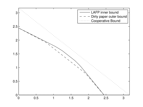
Figure 1: Comparison between an inner bound on the LAFP achievable region and an outer bound on the dirty paper achievable region.

Fig. 1 presents a numerical example where the two approaches are compared. In this example, there are two users (receivers). The transmitter has two antennas ($M=2$) and the receivers have one antenna each $(N_{1}=N_{2}=1)$. The power constraint is $P_{TOT}=10$. The distributions of the channel matrices are given by,

$$H^{(1)}=\cases{[1,0.4]&with probability 1/2\cr[1,3]&with probability 1/2}\quad H^{(2)}=\cases{[0.4,1]&with probability 1/2\cr[3,1]&with probability 1/2}$$

The noise variance at each receiver is $1$.

The achievable regions in both cases (i.e. LAFP and dirty-paper) were found by first applying a grid search for the matrices $\Sigma_{X}^{(1)}$ and $\Sigma_{X}^{(2)}$. In line with Theorem 2, we assumed without loss of optimality that the two signals ${\bf X}^{(1)}$ and ${\bf X}^{(2)}$ are independent.

For each such pair $\Sigma_{X}^{(1)}$ and $\Sigma_{X}^{(2)}$, the matrix ${\bf F}$ for user 2 was computed as described above. That is, for the LAFP achievable region, ${\bf F}$ was found by maximizing the achievable rate of user 2 over the set ${\cal F}$ (which is a function of the user’s covariance matrix $\Sigma_{X}^{(2)}$). For the dirty-paper achievable region, ${\bf F}_{DPC}({\mathrm{E}}H)$ was used.

With both schemes, for fixed matrices $\Sigma_{X}^{(1)}$, $\Sigma_{X}^{(2)}$ and ${\bf F}$, the achievable rates $R_{1}$ and $R_{2}$ for the two users were computed as follows. $R_{1}$ was obtained using the following expression (recall that user 1’s observed signal $Y^{(1)}$ is scalar in this example),

$$R_{1}=\frac{1}{2}E_{H^{(1)}}\log\left(1+\frac{H^{(1)}\Sigma_{X}^{(1)}H^{(1)T}}{H^{(1)}\Sigma_{X}^{(2)}H^{(1)T}+1}\right)$$

$R_{2}$ is given by the right hand side of (35). Since we have assumed ${\bf X}^{(1)}$ and ${\bf X}^{(2)}$ to be independent, the expressions for $\Sigma_{U\>|\>S}$ and $\Sigma_{U\>|\>Y,H}({\bf H})$ (which appear in (35)) are simple. That is, $\Sigma_{U\>|\>S}=\Sigma_{X}^{(2)}$ and $\Sigma_{U\>|\>Y,H}({\bf H})$ is obtained from (24) by setting $\Sigma_{S,X}$ to zero.

The maximal sum-rate on the dirty paper outer bound was 2.7 bits per channel use, while the maximum sum-rate on the LAFP inner bound was 2.86. This achievable rate was obtained by selecting,

$$\Sigma_{X}^{(1)}=\left[\begin{array}[]{cc}1&2-\epsilon\\ 2-\epsilon&4\end{array}\right],\quad\Sigma_{X}^{(2)}=\left[\begin{array}[]{cc}4.5&-1.5+\epsilon\\ -1.5+\epsilon&0.5\end{array}\right],\quad{\bf F}=\left[\begin{array}[]{cc}1.0909&0.3636\\ -0.3636&-0.1212\end{array}\right]$$

where $0<\epsilon\rightarrow 0$ such that $\Sigma_{X}^{(1)}$ and $\Sigma_{X}^{(2)}$ are positive definite. Thus, a simple approach, which uses knowledge of the channel distribution at the transmitter, was able to produce at least a 6% increase in throughput.

Although we have not established the optimality of the LAFP achievable region, we can obtain an idea of how far we are from the optimum using a cooperative upper bound on the achievable sum-capacity (i.e., the maximum achievable sum rate to all users), as suggested by Sato [23]. The use of such a bound in the context of the (non-fading) MIMO-BC channel was first suggested by Caire and Shamai [6]. Computation of cooperative upper-bounds for the above fading MIMO-BC example is discussed in Appendix G. We obtained a bound of 3.17 on the maximum achievable sum-rate. Thus, in terms of the sum-rate, LAFP is capable of transmission at rates that are 10% below the optimum.

In Appendix F we will discuss the computation of the LAFP achievable region with more than two users.

V Conclusion

V-A Suggestions for Further Research

1. Heuristic methods for computing ${\bf F}$. Expression (36), with which we computed the matrix ${\bf F}$ for the LAFP region in Sec. IV-B, was developed heuristically. A different expression could possibly produce a substantially larger achievable region. One option would be to search for ${\bf F}$ along a fine grid (as noted in Sec. IV-B). An alternative option would be to apply a gradient ascent method, using ${\bf F}$ as defined in (36) as a starting point.

2. A wider range of strategies. The confinement to linear assignments as defined in Sec. III is in no way known to be optimal. Dupuis $et\,\,al.\,\,$ [11] suggested an algorithm that is based on the concepts of the Blahut-Arimoto algorithm, that can theoretically be used to evaluate the capacity of a general side-information channel (of which the fading paper channel is an instance). In practice, applying the algorithm requires evaluations over a set of strategies which is impossibly large. However, applying the algorithm over any subset of these strategies produces an achievable rate. This achievable rate may further narrow the gap to the cooperative upper-bound (as discussed in Sec. IV-B).

V-B Concluding Remarks

The problem of transmitting over fading MIMO-BC channels is of great practical interest. In this paper we presented an achievable region for this channel that relies on fading-paper transmission strategies. Our main contribution is Theorem 1, which proves that a Gaussian distribution achieves the linear-assignment capacity. We believe that the approach we developed in the proof of that theorem, which employs convex-analysis methods, could be useful in further analysis of this channel.

In Sec. IV-B we have shown that a simple approach, which makes use of the channel distribution information available to the transmitter, easily produces a gain over dirty-paper transmission. Further research (perhaps in the lines of Sec. V-A) could produce further performance gains.

Appendix A The Optimal Achievable Rate with Zero Channel State Information at the Transmitter

Consider a broadcast channel where all the receivers have the same number of antennas. We wish to show that capacity in this case is achieved by time-sharing among the users.

A channel model that assumes zero knowledge of the channel fade to each of the users, effectively assumes that all channels are the same. The signals at the different receivers are equivalent in their statistical properties, and thus each receiver is capable, beside decoding its own signal, of decoding all the messages to the other users as well. Thus, the sum-rate of this system is upper-bounded by the single-user rate of each of the users. Such a capacity region is exhausted by time-sharing.

Appendix B The Optimal Matrix ${\bf F}$ in the Achievability Proof for Dirty-Paper

In this appendix we prove the optimality of ${\bf F}$ as defined by (5). We let ${\bf U}$ and ${\bf X}$ be defined as in the discussion preceding (5). The achievable rate with this choice is given by $I({\bf U};{\bf Y})-I({\bf U},{\bf S})$ (see (4)). We now seek to prove that this rate coincides with the capacity of the corresponding no-interference channel defined by (3). Our proof follows in the lines of a similar proof by Cohen and Lapidoth [6] for the scalar dirty-paper channel.

To obtain our result, we prove a stronger result. We prove that for any choice of $\Sigma_{X}$, letting ${\bf F}$ be given by (5), we obtain that the achievable rate coincides with the achievable rate $I({\bf X};\hat{\bf Y})$ for the no-interference channel (3).

Our objective is to show that the achievable rate $I({\bf U};{\bf Y})-I({\bf U},{\bf S})$, with this choice of ${\bf F}$, coincides with the achievable rate of the no-interference channel when the input ${\bf X}$ is distributed as ${\mathcal{N}}({\bf 0},\Sigma_{X})$.

Let $\hat{\bf X}={\bf W}\hat{\bf Y}$ be the linear minimum mean-square error (LMMSE) estimate for ${\bf X}$ given $\hat{\bf Y}$. ${\bf W}$ is obtained by [19],

$${\bf W}={\mathrm{Cov}}({\bf X},\hat{\bf Y}){\mathrm{Cov}}(\hat{\bf Y})^{-1}=\Sigma_{X}{\bf H}^{T}({\bf H}\Sigma_{X}{\bf H}^{T}+\Sigma_{Z})^{-1}$$ (38)

By definition of the LMMSE estimate, the error ${\bf E}\>{\stackrel{{\scriptstyle\scriptscriptstyle\Delta}}{{=}}}\>{\bf X}-\hat{\bf X}$ is uncorrelated with $\hat{\bf Y}$. Since ${\bf E}$ and $\hat{\bf Y}$ are jointly-Gaussian, they are also independent. ${\bf S}$ is independent of both, and thus ${\bf E}$ is independent of ${\bf Y}=\hat{\bf Y}+{\bf H}{\bf S}$.

Examining $I({\bf U};{\bf Y})-I({\bf U},{\bf S})$, we have

$$I({\bf U};{\bf Y})-I({\bf U},{\bf S})=h({\bf U}\>|\>{\bf S})-h({\bf U}\>|\>{\bf Y})$$ (39)

We now examine both elements of the difference on the right hand side of the above.

$$h({\bf U}\>|\>{\bf S})=h({\bf F}{\bf S}+{\bf X}\>|\>{\bf S})=h({\bf X})$$ (40)

where the last equation is obtained by the fact that ${\bf S}$ and ${\bf X}$ are independent.

$$h({\bf U}\>|\>{\bf Y}) = h({\bf F}{\bf S}+{\bf X}\>|\>{\bf Y})\>{\stackrel{{\scriptstyle(a)}}{{=}}}\>h({\bf W}{\bf H}{\bf S}+{\bf X}\>|\>{\bf Y})$$ (41)

$$= h({\bf W}{\bf H}{\bf S}+{\bf X}-{\bf W}{\bf Y}\>|\>{\bf Y})=h({\bf W}{\bf H}{\bf S}+{\bf X}-{\bf W}({\bf H}{\bf S}+{\bf H}{\bf X}+{\bf Z})\>|\>{\bf Y})$$

$$= h({\bf X}-{\bf W}({\bf H}{\bf X}+{\bf Z})\>|\>{\bf Y})=h({\bf X}-\hat{\bf X}\>|\>{\bf Y})=h({\bf E}\>|\>{\bf Y})\>{\stackrel{{\scriptstyle(b)}}{{=}}}\>h({\bf E})\>{\stackrel{{\scriptstyle(c)}}{{=}}}\>h({\bf E}\>|\>\hat{\bf Y})$$

$$= h({\bf X}-{\bf W}\hat{\bf Y}\>|\>\hat{\bf Y})=h({\bf X}\>|\>\hat{\bf Y})$$

Equality (a) is obtained from the observation that the right hand side of (5) equals ${\bf W}\cdot{\bf H}$ where ${\bf W}$ is given by (38). Equalities (b) and (c) are obtained from the fact that ${\bf E}$ is independent of $\hat{\bf Y}$ and ${\bf Y}$. Finally, combining (39), (40) and (41) we obtain our desired result,

$$I({\bf U};{\bf Y})-I({\bf U},{\bf S})=h({\bf X})-h({\bf X}\>|\>\hat{\bf Y})=I({\bf X};\hat{\bf Y})$$

∎

Appendix C Proof of Lemma 1

Let $q$ and $Q$ be a pair of feasible functions for (12). We will now show that $F(q,Q)\leq F({q^{\star}},{Q^{\star}})$.

$$F(q,Q)-F({q^{\star}},{Q^{\star}}) = \int_{{\bf s}\in\mbox{\boldlarge R}^{M}}\int_{{\bf u}\in\mbox{\boldlarge R}^{M}}\int_{{\bf y}\in\mbox{\boldlarge R}^{N}}\int_{{\bf H}\in{\cal R}_{H}}f({\bf s})f({\bf y},{\bf H}\>|\>{\bf s},{\bf x}={\bf f}({\bf u},{\bf s}))\cdot$$ (42)

$$\cdot\left[q({\bf u}\>|\>{\bf s})\log\frac{Q({\bf u}\>|\>{\bf y},{\bf H})}{q({\bf u}\>|\>{\bf s})}-{q^{\star}}({\bf u}\>|\>{\bf s})\log\frac{{Q^{\star}}({\bf u}\>|\>{\bf y},{\bf H})}{{q^{\star}}({\bf u}\>|\>{\bf s})}\right]{\>d\bf H}{\>d\bf y}{\>d\bf u}{\>d\bf s}$$

Let $l(x,y)\>{\stackrel{{\scriptstyle\scriptscriptstyle\Delta}}{{=}}}\>x\cdot\log(y/x)$. This function is jointly-concave in its arguments. By the gradient inequality [4][Chapter 3, Section 3.1.3] for concave functions, we have for arbitrary $x,y\in\mbox{\boldlarge R}_{+}$ and ${x^{\star}},{y^{\star}}\in\mbox{\boldlarge R}_{++}$,

$$l(x,y)-l({x^{\star}},{y^{\star}})\leq l_{x}({x^{\star}},{y^{\star}})\cdot(x-{x^{\star}})+l_{y}({x^{\star}},{y^{\star}})\cdot(y-{y^{\star}})$$

where $l_{x}$ and $l_{y}$ denote the partial derivatives of $l$ with respect to $x$ and $y$, respectively. Thus, we can bound (42) by,

$$F(q,Q)-F({q^{\star}},{Q^{\star}}) \leq \int_{{\bf s}\in\mbox{\boldlarge R}^{M}}\int_{{\bf u}\in\mbox{\boldlarge R}^{M}}\int_{{\bf y}\in\mbox{\boldlarge R}^{N}}\int_{{\bf H}\in{\cal R}_{H}}f({\bf s})f({\bf y},{\bf H}\>|\>{\bf s},{\bf x}={\bf f}({\bf u},{\bf s}))\cdot$$ (43)

$$\cdot [l_{x}({q^{\star}}({\bf u}\>|\>{\bf s}),{Q^{\star}}({\bf u}\>|\>{\bf y},{\bf H}))\cdot(q({\bf u}\>|\>{\bf s})-{q^{\star}}({\bf u}\>|\>{\bf s}))+$$

$$+ l_{y}({q^{\star}}({\bf u}\>|\>{\bf s}),{Q^{\star}}({\bf u}\>|\>{\bf y},{\bf H}))\cdot(Q({\bf u}\>|\>{\bf y},{\bf H})-{Q^{\star}}({\bf u}\>|\>{\bf y},{\bf H}))]{\>d\bf H}{\>d\bf y}{\>d\bf u}{\>d\bf s}$$

In the development below, we will show that this integral equals zero. This will then conclude the proof of the lemma.

To prove this, we will show that the two integrals below equal zero. For simplicity of notation, we let $q$ and $Q$ denote $q({\bf u}\>|\>{\bf s})$ and $Q({\bf u}\>|\>{\bf y},{\bf H})$, respectively.

$$\int_{{\bf s}\in\mbox{\boldlarge R}^{M}}\int_{{\bf u}\in\mbox{\boldlarge R}^{M}}\int_{{\bf y}\in\mbox{\boldlarge R}^{N}}\int_{{\bf H}\in{\cal R}_{H}}f({\bf s})f({\bf y},{\bf H}\>|\>{\bf s},{\bf x}={\bf f}({\bf u},{\bf s}))\cdot l_{x}({q^{\star}},{Q^{\star}})\cdot(q-{q^{\star}}){\>d\bf H}{\>d\bf y}{\>d\bf u}{\>d\bf s} = 0$$ (44)

$$\int_{{\bf s}\in\mbox{\boldlarge R}^{M}}\int_{{\bf u}\in\mbox{\boldlarge R}^{M}}\int_{{\bf y}\in\mbox{\boldlarge R}^{N}}\int_{{\bf H}\in{\cal R}_{H}}f({\bf s})f({\bf y},{\bf H}\>|\>{\bf s},{\bf x}={\bf f}({\bf u},{\bf s}))\cdot l_{y}({q^{\star}},{Q^{\star}})\cdot(Q-{Q^{\star}}){\>d\bf H}{\>d\bf y}{\>d\bf u}{\>d\bf s} = 0$$ (45)

We first prove (44). Multiplying (17) by $q-{q^{\star}}$, and using the fact that $l_{x}(x,y)=\log(y/x)-1$, we get

$$\left[\int_{{\bf y}\in\mbox{\boldlarge R}^{N}}\int_{{\bf H}\in{\cal R}_{H}}f({\bf s})f({\bf y},{\bf H}\>|\>{\bf s},{\bf x}={\bf f}({\bf u},{\bf s}))l_{x}({q^{\star}},{Q^{\star}}){\>d\bf H}{\>d\bf y}\right](q-{q^{\star}})+$$

$$\quad\left[f({\bf s})<\Upsilon,{\bf f}({\bf u},{\bf s})\cdot{\bf f}({\bf u},{\bf s})^{T}>\right](q-{q^{\star}})+\left[f({\bf s})<\Gamma,{\bf s}\cdot{\bf f}({\bf u},{\bf s})^{T}>\right](q-{q^{\star}})+\alpha({\bf s})(q-{q^{\star}})=0$$

$$\quad\quad\quad\quad\quad\quad\quad\quad\quad\quad\quad\quad\quad\quad\quad\quad\quad\quad\quad\quad\quad\quad\quad\quad\quad\quad\quad\quad\quad\forall{\bf s}\in\mbox{\boldlarge R}^{M},\forall{\bf u}\in\mbox{\boldlarge R}^{M}$$

Integrating the above with respect to ${\bf u}$ and ${\bf s}$ would yield zero. We now focus on the integrals of the individual elements of the above sum. The first integral is equal to the left hand side of (44). To prove this integral is zero, we will show that the other integrals are zero. This will yield (44).

We first integrate with respect to ${\bf u}$ and then ${\bf s}$. The order of integration matters, because the range of the integration is unbounded, and some of the integrands are not non-negative and not necessarily Lebesgue-integrable (i.e., the integral of their absolute value may be infinite).

$$\int_{{\bf s}\in\mbox{\boldlarge R}^{M}}\int_{{\bf u}\in\mbox{\boldlarge R}^{M}}\left[f({\bf s})<\Upsilon,{\bf f}({\bf u},{\bf s})\cdot{\bf f}({\bf u},{\bf s})^{T}>\right](q-{q^{\star}}){\>d\bf u}{\>d\bf s}$$

$$\quad=<\Upsilon,\int_{{\bf s}\in\mbox{\boldlarge R}^{M}}\int_{{\bf u}\in\mbox{\boldlarge R}^{M}}f({\bf s})\left[{\bf f}({\bf u},{\bf s})\cdot{\bf f}({\bf u},{\bf s})^{T}\right]\cdot q{\>d\bf u}{\>d\bf s}$$

$$\quad-\int_{{\bf s}\in\mbox{\boldlarge R}^{M}}\int_{{\bf u}\in\mbox{\boldlarge R}^{M}}f({\bf s})\left[{\bf f}({\bf u},{\bf s})\cdot{\bf f}({\bf u},{\bf s})^{T}\right]\cdot{q^{\star}}{\>d\bf u}{\>d\bf s}>$$

$$\quad=<\Upsilon,\Sigma_{X}-\Sigma_{X}>=0$$

The equality before last results from (13) and from the feasibility of the functions $q$ and ${q^{\star}}$. In a similar way, using (14), we obtain that,

$$\int_{{\bf s}\in\mbox{\boldlarge R}^{M}}\int_{{\bf u}\in\mbox{\boldlarge R}^{M}}\left[f({\bf s})<\Gamma,{\bf s}\cdot{\bf f}({\bf u},{\bf s})^{T}>\right](q-{q^{\star}}){\>d\bf u}{\>d\bf s}=0$$

Finally, we examine the last integral.

$$\int_{{\bf s}\in\mbox{\boldlarge R}^{M}}\int_{{\bf u}\in\mbox{\boldlarge R}^{M}}\alpha({\bf s})(q-{q^{\star}}){\>d\bf u}{\>d\bf s}=\int_{{\bf s}\in\mbox{\boldlarge R}^{M}}\alpha({\bf s})\left[\int_{{\bf u}\in\mbox{\boldlarge R}^{M}}q{\>d\bf u}-\int_{{\bf u}\in\mbox{\boldlarge R}^{M}}{q^{\star}}{\>d\bf u}\right]{\>d\bf s}$$

$$\quad=\int_{{\bf s}\in\mbox{\boldlarge R}^{M}}\alpha({\bf s})\left[1-1\right]{\>d\bf s}=0$$

The equality before last results from (15). Thus, we obtain (44).

Similarly, relying on (18) and (16), we obtain,

$$\int_{{\bf y}\in\mbox{\boldlarge R}^{N}}\int_{{\bf H}\in{\cal R}_{H}}\int_{{\bf u}\in\mbox{\boldlarge R}^{M}}\int_{{\bf s}\in\mbox{\boldlarge R}^{M}}f({\bf s})f({\bf y},{\bf H}\>|\>{\bf s},{\bf x}={\bf f}({\bf u},{\bf s}))\cdot l_{y}({q^{\star}},{Q^{\star}})\cdot(Q-{Q^{\star}}){\>d\bf s}{\>d\bf u}{\>d\bf H}{\>d\bf y}=0$$ (46)

The order of integration, unfortunately, is not that of (45). To prove that we may change the order of integration, we must prove that the integrand is Lebesgue-integrable (Fubini’s Theorem, see e.g. [2][Theorem 18.3]). To do this, we will prove that

$$\int_{{\bf y}\in\mbox{\boldlarge R}^{N}}\int_{{\bf H}\in{\cal R}_{H}}\int_{{\bf u}\in\mbox{\boldlarge R}^{M}}\int_{{\bf s}\in\mbox{\boldlarge R}^{M}}f({\bf s})f({\bf y},{\bf H}\>|\>{\bf s},{\bf x}={\bf f}({\bf u},{\bf s}))\cdot l_{y}({q^{\star}},{Q^{\star}})\cdot Q{\>d\bf s}{\>d\bf u}{\>d\bf H}{\>d\bf y}<\infty$$ (47)

Since the integrand in the above is nonnegative, this would yield that it is integrable. Since $Q$ is arbitrary, the same would apply if we replace it with ${Q^{\star}}$. The integrand in (46), which is not necessarily nonnegative, is thus also integrable because it is obtained by subtracting the integrand in (47) by the same expression, with $Q$ replaced by ${Q^{\star}}$.

Using $l_{y}(x,y)=x/y$, we may rewrite the left hand side of (47) as

$$\int_{{\bf y}\in\mbox{\boldlarge R}^{N}}\int_{{\bf H}\in{\cal R}_{H}}\int_{{\bf u}\in\mbox{\boldlarge R}^{M}}\int_{{\bf s}\in\mbox{\boldlarge R}^{M}}f({\bf s})f({\bf y},{\bf H}\>|\>{\bf s},{\bf x}={\bf f}({\bf u},{\bf s}))\cdot\frac{{q^{\star}}}{{Q^{\star}}}\cdot Q{\>d\bf s}{\>d\bf u}{\>d\bf H}{\>d\bf y}$$

$$\quad=\int_{{\bf y}\in\mbox{\boldlarge R}^{N}}\int_{{\bf H}\in{\cal R}_{H}}\int_{{\bf u}\in\mbox{\boldlarge R}^{M}}\frac{Q}{{Q^{\star}}}\cdot\left[\int_{{\bf s}\in\mbox{\boldlarge R}^{M}}f({\bf s})f({\bf y},{\bf H}\>|\>{\bf s},{\bf x}={\bf f}({\bf u},{\bf s}))\cdot{q^{\star}}{\>d\bf s}\right]{\>d\bf u}{\>d\bf H}{\>d\bf y}$$ (48)

The inside of the brackets is equal to ${q^{\star}}({\bf y},{\bf H},{\bf u})$, defined to equal the marginal density of ${\bf Y}$, ${\bf H}$ and ${\bf U}$ where the distribution of ${\bf U}$ given ${\bf S}$ is determined by the density ${q^{\star}}$. Similarly defining ${q^{\star}}({\bf y},{\bf H})$, we obtain by the conditions of Lemma 1, that ${q^{\star}}({\bf y},{\bf H},{\bf u})={q^{\star}}({\bf y},{\bf H})\cdot{Q^{\star}}({\bf u}\>|\>{\bf y},{\bf H})$. Thus, (48) becomes,

$$\int_{{\bf y}\in\mbox{\boldlarge R}^{N}}\int_{{\bf H}\in{\cal R}_{H}}\int_{{\bf u}\in\mbox{\boldlarge R}^{M}}\frac{Q}{{Q^{\star}}}\cdot{q^{\star}}({\bf y},{\bf H})\cdot{Q^{\star}}{\>d\bf u}{\>d\bf H}{\>d\bf y}=\int_{{\bf y}\in\mbox{\boldlarge R}^{N}}\int_{{\bf H}\in{\cal R}_{H}}{q^{\star}}({\bf y},{\bf H})\int_{{\bf u}\in\mbox{\boldlarge R}^{M}}Q{\>d\bf u}{\>d\bf H}{\>d\bf y}$$

$$\quad=\int_{{\bf y}\in\mbox{\boldlarge R}^{N}}\int_{{\bf H}\in{\cal R}_{H}}{q^{\star}}({\bf y},{\bf H})\cdot 1{\>d\bf H}{\>d\bf y}=1<\infty$$

Thus, by the above discussion, the order of integration in (46) can be changed, and we obtain (45). Coupled with (44), this proves that the right hand side of (43) is zero, concluding the proof of the lemma. ∎

Appendix D The Achievability of $F(q_{G},Q_{G})$

The random variables ${\bf U},{\bf S},{\bf Y},H$ that achieve the LAFP capacity are continuous. In practice one can only realize the Gelfand-Pinsker capacity of a set $\hat{{\bf U}},\hat{{\bf S}},\hat{{\bf Y}},\hat{H}$ of discrete random variables. We now show that ${\bf U},{\bf S},{\bf Y},H$ can be quantized to a set $\hat{{\bf U}},\hat{{\bf S}},\hat{{\bf Y}},\hat{H}$ of discrete random variables that can approach the LAFP capacity arbitrarily close. The LAFP capacity is given by $R_{\rm achievable}=F(q_{G},Q_{G})$ where $F(q,Q)$ is defined by (11).

We create a quantized version as follows. Let ${\cal B}_{n}(c,d)$ denote a cube in $\mbox{\boldlarge R}^{n}$ with center $c$ and size length $d$, i.e.,

$${\cal B}_{n}(c,d)=\left\{(x_{1},x_{2},\ldots,x_{n})\>:\>c-d/2<x_{i}\leq c+d/2,\>i=1,\ldots,n\right\}$$

We define discrete random variables $\hat{{\bf S}},\hat{{\bf U}},\hat{{\bf Y}},\hat{H}$ which are quantized versions of ${{\bf S}},{{\bf U}},{{\bf Y}},{H}$, respectively, as follows. Recall that $M$ and $N$ are the dimensions of ${\bf S}$ and ${\bf Y}$, respectively. The dimension of $H$ is thus $M\times N$. Fix some $\epsilon>0$ sufficiently small, and $\rho>0$ sufficiently large. Let ${\bf s}_{i}$, $i=1,\ldots,N_{s}$ denote all the points in $\mbox{\boldlarge R}^{M}$, such that ${\bf s}_{i}\in{\cal B}_{M}(0,\rho)$ and such that all the coordinates of ${\bf s}_{i}$ are integer multiples of $\epsilon$. Similarly, let ${\bf u}_{j}$, $j=1,\ldots,N_{u}$, ${\bf y}_{k}$, $k=1,\ldots,N_{y}$ and ${\bf H}_{l}$, $l=1,\ldots,N_{h}$ denote all the points in $\mbox{\boldlarge R}^{M}$, $\mbox{\boldlarge R}^{N}$ and ${\cal R}_{H}$, such that ${\bf u}_{j}\in{\cal B}_{M}(0,\rho)$, ${\bf y}_{k}\in{\cal B}_{N}(0,\rho)$ and ${\bf H}_{l}\in{\cal B}_{MN}(0,\rho)$, and such that all the coordinates of ${\bf u}_{j}$, ${\bf y}_{k}$ and ${\bf H}_{l}$ are integer multiples of $\epsilon$.

We define by ${\cal S}_{i}$, $i=0,1,\ldots,N_{s}$ the following regions,

$${\cal S}_{i}=\left\{\begin{array}[]{ll}\mbox{\boldlarge R}^{M}\bigcap{\cal B}_{M}({\bf s}_{i},\epsilon),&\hbox{if $i=1,2,\ldots,N_{s}$;}\\ \mbox{\boldlarge R}^{M}\setminus\left[{\bigcup_{i=1}^{N_{s}}{\cal B}_{M}({\bf s}_{i},\epsilon)}\right],&\hbox{if $i=0$.}\end{array}\right.$$

Similarly we define

$${\cal U}_{j}=\left\{\begin{array}[]{ll}\mbox{\boldlarge R}^{M}\bigcap{\cal B}_{M}({\bf u}_{j},\epsilon),&\hbox{if $j=1,2,\ldots,N_{u}$;}\\ \mbox{\boldlarge R}^{M}\setminus\left[{\bigcup_{j=1}^{N_{u}}{\cal B}_{M}({\bf u}_{j},\epsilon)}\right],&\hbox{if $j=0$.}\end{array}\right.$$

$${\cal Y}_{k}=\left\{\begin{array}[]{ll}{\cal B}_{N}({\bf y}_{k},\epsilon),&\hbox{if $k=1,2,\ldots,N_{y}$;}\\ \mbox{\boldlarge R}^{N}\setminus{\bigcup_{k=1}^{N_{y}}{\cal B}_{N}({\bf y}_{k},\epsilon)},&\hbox{if $k=0$.}\end{array}\right.$$

and

$${\cal H}_{l}=\left\{\begin{array}[]{ll}{\cal R}_{H}\bigcap{\cal B}_{MN}({\bf H}_{l},\epsilon),&\hbox{if $l=1,2,\ldots,N_{h}$;}\\ {\cal R}_{H}\setminus{\bigcup_{l=1}^{N_{h}}{\cal B}_{MN}({\bf H}_{l},\epsilon)},&\hbox{if $l=0$.}\end{array}\right.$$

The quantized random variable $\hat{{\bf S}}$ is defined as follows: $\hat{{\bf S}}=i$ if ${\bf S}\in{\cal S}_{i}$. The quantized random variables $\hat{{\bf U}}$, $\hat{{\bf Y}}$ and $\hat{H}$ are defined similarly. The joint probability of $\hat{{\bf S}},\hat{{\bf U}},\hat{{\bf Y}},\hat{H}$ is,

$$P\left(\hat{{\bf S}}=i,\hat{{\bf U}}=j,\hat{{\bf Y}}=k,\hat{H}=l\right)=$$

$$\int_{{\bf s}\in{\cal S}_{i}}\int_{{\bf u}\in{\cal U}_{j}}\int_{{\bf y}\in{\cal Y}_{k}}\int_{{\bf H}\in{\cal H}_{l}}f({\bf s})f({\bf y},{\bf H}\>|\>{\bf s},{\bf x}={\bf}({\bf s},{\bf u}))q_{G}({\bf u}\>|\>{\bf s})\>d{\bf H}\>d{{\bf y}}\>d{{\bf u}}\>d{{\bf s}}$$

The Gelfand-Pinsker achievable rate corresponding to the quantized random variables is,

$$\hat{R}=\sum_{i,j,k,l}P\left(\hat{{\bf S}}=i,\hat{{\bf U}}=j,\hat{{\bf Y}}=k,\hat{H}=l\right)\log\frac{P(\hat{{\bf U}}=j\>|\>\hat{{\bf Y}}=k,\hat{H}=l)}{P(\hat{{\bf U}}=j\>|\>\hat{{\bf S}}=i)}$$ (49)

We claim that $\hat{R}=R_{\rm achievable}+o_{\epsilon,\rho}(1)$ where $o_{\epsilon,\rho}(1)$ is a term that approaches $0$ as $\epsilon\rightarrow 0$ and $\rho\rightarrow\infty$.

To see this, first note that when ${\bf s}\in{\cal S}_{0}$ or ${\bf u}\in{\cal U}_{0}$ or ${\bf y}\in{\cal Y}_{0}$ or ${\bf H}\in{\cal H}_{0}$, the contribution to $F(q_{G},Q_{G})$ in (11) approaches $0$ as $\rho\rightarrow\infty$. In addition, $\log\frac{Q_{G}({\bf u}\>|\>{\bf y},{\bf H})}{q_{G}({\bf u}\>|\>{\bf s})}$ is uniformly continuous in the region ${\bf s}\in\overline{{\cal S}_{0}}$, ${\bf u}\in\overline{{\cal U}_{0}}$, ${\bf y}\in\overline{{\cal Y}_{0}}$, ${\bf H}\in\overline{{\cal H}_{0}}$. Hence,

$$F(q_{G},Q_{G})=\sum_{i\neq 0,j\neq 0,k\neq 0,l\neq 0}P\left(\hat{{\bf S}}=i,\hat{{\bf U}}=j,\hat{{\bf Y}}=k,\hat{H}=l\right)\log\frac{Q_{G}({\bf u}_{j}\>|\>{\bf y}_{k},{\bf H}_{l})}{q_{G}({\bf u}_{j}\>|\>{\bf s}_{i})}+o_{\epsilon,\rho}(1)$$

In addition, by the uniform continuity of the Gaussian distribution in the region ${\bf s}\in\overline{{\cal S}_{0}}$, ${\bf u}\in\overline{{\cal U}_{0}}$, ${\bf y}\in\overline{{\cal Y}_{0}}$, ${\bf H}\in\overline{{\cal H}_{0}}$,

$$\frac{P(\hat{{\bf U}}=j\>|\>\hat{{\bf Y}}=k,\hat{H}=l)}{Q_{G}({\bf u}_{j}\>|\>{\bf y}_{k},{\bf H}_{l})}=1+o_{\epsilon,\rho}(1)$$

and

$$\frac{P(\hat{{\bf U}}=j\>|\>\hat{{\bf s}}=i)}{q_{G}({\bf u}_{j}\>|\>{\bf s}_{i})}=1+o_{\epsilon,\rho}(1)$$

Finally by arguments similar to those indicated above, the contribution of terms with $i=0$ or $j=0$ or $k=0$ or $l=0$ in (49) is negligible.

Hence we obtained the desired claim that $\hat{R}=R_{\rm achievable}+o_{\epsilon,\rho}(1)$.

Appendix E Proof of Theorem 2

Our approach is the following. We begin with an assignment of variables for the LAFP achievable region. This means a set of variables ${\bf X}_{1}$,…,${\bf X}_{L}$ that are not necessarily independent. A set of matrices ${\bf F}_{1},...,{\bf F}_{L}$ and a set of auxiliary random variables ${\bf U}_{l}={\bf F}_{l}{\bf S}_{l}+{\bf X}_{l}$ where ${\bf S}_{l}=\Sigma_{i<l}{\bf X}_{i}$. Recall that in our current context, ${\bf X}={\bf X}_{1}+...+{\bf X}_{L}$ denotes the transmitted symbol of the MIMO-BC channel, while ${\bf X}_{l}$ denotes the transmitted signal to user $l$, equivalent to ${\bf X}$ as in Sec. III-B.

We will construct an alternative set of independent random variables $\hat{\bf X}_{1},...\hat{\bf X}_{L}$ and $\hat{\bf F}_{1},...,\hat{\bf F}_{L}$ such that the transmitted signal $\hat{\bf X}\>{\stackrel{{\scriptstyle\scriptscriptstyle\Delta}}{{=}}}\>\hat{\bf X}_{1}+...+\hat{\bf X}_{L}={\bf X}_{1}+...+{\bf X}_{L}={\bf X}$. Thus, the distribution of the actual transmitted signal is unchanged and satisfies the power constraint. Furthermore, we show that for similarly defined ${\bf{\hat{U}}}_{l}=\hat{\bf F}_{l}{\bf{\hat{S}}}_{l}+\hat{\bf X}_{l}$ and ${\bf{\hat{S}}}_{l}=\Sigma_{i<l}\hat{\bf X}_{i}$, the achievable rates satisfy $\hat{R}_{l}\geq R_{l}$, where

$$\hat{R}_{l}\>{\stackrel{{\scriptstyle\scriptscriptstyle\Delta}}{{=}}}\>I({\bf{\hat{U}}}_{l};{\bf Y}_{l},{\bf H}_{l})-I({\bf{\hat{U}}}_{l};{\bf{\hat{S}}}_{l}),\quad\quad R_{l}=I({\bf U}_{l};{\bf Y}_{l},{\bf H}_{l})-I({\bf U}_{l};{\bf S}_{l})$$

E-A Definition of $\hat{\bf X}_{1},...,\hat{\bf X}_{L}$

For each $l=1,...,L$, using Gram-Schmidt orthogonalization, ${\bf X}_{l}$ can be written as ${\bf X}_{l}=\Gamma_{l}{\bf S}_{l}+{\bf X}^{\prime}_{l}$ where $\Gamma_{l}$ is a matrix and where ${\bf S}_{l}$ and ${\bf X}^{\prime}_{l}$ are uncorrelated. Therefore, since we have assumed, in our definition of the LAFP region in Sec. IV-A, that all variables are jointly Gaussian, they are independent. With this definition,

$${\bf X} = {\bf S}_{L}+{\bf X}_{L}=({\bf I}+\Gamma_{L}){\bf S}_{L}+{\bf X}^{\prime}_{L}$$

$$= ({\bf I}+\Gamma_{L})\left[{\bf S}_{L-1}+{\bf X}_{L-1}\right]+{\bf X}^{\prime}_{L}=({\bf I}+\Gamma_{L})\left[({\bf I}+\Gamma_{L-1}){\bf S}_{L-1}+{\bf X}^{\prime}_{L-1}\right]+{\bf X}^{\prime}_{L}$$

$$...$$

$$= ({\bf I}+\Gamma_{L})\cdot...\cdot({\bf I}+\Gamma_{2}){\bf X}^{\prime}_{1}+({\bf I}+\Gamma_{L})\cdot...\cdot({\bf I}+\Gamma_{3}){\bf X}^{\prime}_{2}+...+({\bf I}+\Gamma_{L}){\bf X}^{\prime}_{L-1}+{\bf X}^{\prime}_{L}$$

We thus define $\hat{\bf X}_{l}={\bf{G}}_{l}{\bf X}^{\prime}_{l}$ where ${\bf{G}}_{l}=({\bf I}+\Gamma_{L})\cdot...\cdot({\bf I}+\Gamma_{l+1})$ $l=1,...,L-1$, ${\bf{G}}_{L}={\bf I}$. By construction, $\sum_{l=1}^{L}\hat{\bf X}_{l}={\bf X}=\sum_{l=1}^{L}{\bf X}_{l}$, as desired.

The following lemma summarized some properties of our random variables.

Lemma 2

For all $l=1,...,L$,

1. $\hat{\bf X}_{l}$ is independent of ${\bf X}_{1},...,{\bf X}_{l-1}$.

2. $\hat{\bf X}_{l}$ is independent of ${\bf S}_{1},...,{\bf S}_{l}$.

3. $\hat{\bf X}_{l}$ is independent of $\hat{\bf X}_{1},...,\hat{\bf X}_{l-1}$.

4. ${\bf{\hat{S}}}_{l}=G_{l-1}{\bf S}_{l}$

Proof: To prove property 1, observe that the following Markov relations hold: ${\bf X}_{1},...,{\bf X}_{l-1}\longleftrightarrow{\bf S}_{l}\longleftrightarrow{\bf S}_{l},{\bf X}_{l}\longleftrightarrow\hat{\bf X}_{l}$. $\hat{\bf X}_{l}$, by construction, is independent of ${\bf S}_{l}$. It is thus straightforward to verify, using this Markov relation, that it is also independent of ${\bf X}_{1},...,{\bf X}_{l-1}$. To obtain properties 2 and 3, observe that ${\bf S}_{1},...,{\bf S}_{l}$ and $\hat{\bf X}_{1},...,\hat{\bf X}_{l-1}$ are functions of ${\bf X}_{1},...,{\bf X}_{l-1}$ and thus are independent of $\hat{\bf X}_{l}$.

The last property is easily obtained by induction. For $l=1$,

$${\bf{\hat{S}}}_{1}=\sum_{i<1}\hat{\bf X}_{i}={\bf 0}=\sum_{i<1}{\bf X}_{i}={\bf S}_{1}$$

The rest is obtained by the following induction:

$${\bf{\hat{S}}}_{l+1} = {\bf{\hat{S}}}_{l}+\hat{\bf X}_{l}=G_{l-1}{\bf S}_{l}+G_{l}{\bf X}^{\prime}_{l}=G_{l}(I+\Gamma_{l}){\bf S}_{l}+G_{l}{\bf X}^{\prime}_{l}=G_{l}\left[(I+\Gamma_{l}){\bf S}_{l}+{\bf X}^{\prime}_{l}\right]$$

$$= G_{l}\left[{\bf S}_{l}+\Gamma_{l}{\bf S}_{l}+{\bf X}^{\prime}_{l}\right]=G_{l}\left[{\bf S}_{l}+{\bf X}_{l}\right]=G_{l}{\bf S}_{l+1}$$

∎

E-B Definition of $\hat{\bf F}_{1},...,\hat{\bf F}_{L}$

We have not yet defined $\hat{\bf F}_{l}$. To do so, we first consider ${\bf{G}}_{l}\cdot{\bf U}_{l}$. By the definition of ${\bf U}_{l}$

$${\bf{G}}_{l}\cdot{\bf U}_{l}={\bf{G}}_{l}[{\bf F}_{l}{\bf S}_{l}+{\bf X}_{l}]={\bf{G}}_{l}[({\bf F}_{l}+\Gamma_{l}){\bf S}_{l}+{\bf X}^{\prime}_{l}]={\bf{G}}_{l}({\bf F}_{l}+\Gamma_{l}){\bf S}_{l}+\hat{\bf X}_{l}$$ (50)

where the last inequality was obtained by the definition of $\hat{\bf X}_{l}$, above. Using Gram-Schmidt orthogonalization, ${\bf S}_{l}$ can be written as ${\bf S}_{l}={\bf B}_{l}\cdot{\bf{\hat{S}}}_{l}+{\bf D}_{l}$ where ${\bf B}_{l}$ is a matrix and ${\bf D}_{l}$ is uncorrelated with ${\bf{\hat{S}}}_{l}$. Since the variables are jointly Gaussian, ${\bf D}_{l}$ is also independent of ${\bf{\hat{S}}}_{l}$. We proceed

$${\bf{G}}_{l}\cdot{\bf U}_{l} = {\bf{G}}_{l}({\bf F}_{l}+\Gamma_{l})[{\bf B}_{l}{\bf{\hat{S}}}_{l}+{\bf D}_{l}]+\hat{\bf X}_{l}$$ (51)

$$= {\bf{G}}_{l}({\bf F}_{l}+\Gamma_{l}){\bf B}_{l}{\bf{\hat{S}}}_{l}+\hat{\bf X}_{l}+{\bf{G}}_{l}({\bf F}_{l}+\Gamma_{l}){\bf D}_{l}$$

We define $\hat{\bf F}_{l}={\bf{G}}_{l}({\bf F}_{l}+\Gamma_{l}){\bf B}_{l}$.

E-C Proof of $\hat{R}_{l}>R_{l}$

Recall that ${\bf{\hat{U}}}_{l}=\hat{\bf F}_{l}{\bf{\hat{S}}}_{l}+\hat{\bf X}_{l}$. To prove $\hat{R}_{l}>R_{l}$, we first define an intermediate auxiliary variable ${\bf{\tilde{U}}}_{l}={\bf{G}}_{l}\cdot{\bf U}_{l}$. Since ${\bf{\tilde{U}}}_{l}$ is a function of ${\bf U}_{l}$, we have

$$R_{l} = I({\bf{\tilde{U}}}_{l},{\bf U}_{l};{\bf Y}_{l},H_{l})-I({\bf{\tilde{U}}}_{l},{\bf U}_{l};{\bf S}_{l})$$

$$= H({\bf{\tilde{U}}}_{l},{\bf U}_{l}\>|\>{\bf S}_{l})-H({\bf{\tilde{U}}}_{l},{\bf U}_{l}\>|\>{\bf Y}_{l},H_{l})$$

$$= H({\bf{\tilde{U}}}_{l}\>|\>{\bf S}_{l})-H({\bf{\tilde{U}}}_{l}\>|\>{\bf Y}_{l},H_{l})+H({\bf U}_{l}\>|\>{\bf{\tilde{U}}}_{l},{\bf S}_{l})-H({\bf U}_{l}\>|\>{\bf{\tilde{U}}}_{l},{\bf Y}_{l},H_{l})$$

$$= \left[H({\bf{\tilde{U}}}_{l}\>|\>{\bf S}_{l})-H({\bf{\tilde{U}}}_{l}\>|\>{\bf Y}_{l},H_{l})\right]+\left[I({\bf U}_{l};{\bf{\tilde{U}}}_{l},{\bf Y}_{l},H_{l})-I({\bf U}_{l};{\bf{\tilde{U}}}_{l},{\bf S}_{l})\right]$$

We now wish to show that the contents of the second brackets are non-positive. For this purpose, we will show that the following Markov relations hold: ${\bf U}_{l}\longleftrightarrow{\bf{\tilde{U}}}_{l},{\bf S}_{l}\longleftrightarrow{\bf{\tilde{U}}}_{l},\hat{\bf X}_{l},{\bf{\hat{S}}}_{l}\longleftrightarrow{\bf{\tilde{U}}}_{l},{\bf X}\longleftrightarrow{\bf{\tilde{U}}}_{l},{\bf Y}_{l},H_{l}$. The desired result will then follow from the first and last Markov relations, using the data processing inequality.

The second relation (first Markov triple) follows from the fact that $\hat{\bf X}_{l}$ and ${\bf{\hat{S}}}_{l}$ may be determined from ${\bf{\tilde{U}}}_{l}$ and ${\bf S}_{l}$ by means of deterministic functions: $\hat{\bf X}_{l}$ through (50), and ${\bf{\hat{S}}}_{l}$, by Lemma 2 satisfies ${\bf{\hat{S}}}_{l}={\bf{G}}_{l-1}{\bf S}_{l}$. For the third relation, observe that ${\bf X}={\bf{\hat{S}}}_{l}+\hat{\bf X}_{l}+\sum_{i>l}\hat{\bf X}_{i}$. By the above definition all $\{\hat{\bf X}_{i}\}_{i>l}$, are independent of ${\bf U}_{l},{\bf{\tilde{U}}}_{l},{\bf{\hat{S}}}_{l},{\bf S}_{l}$ and $\hat{\bf X}_{l}$. Therefore this Markov relation holds. The last Markov relation is straightforward.

We thus have,

$$R_{l}\leq H({\bf{\tilde{U}}}_{l}\>|\>{\bf S}_{l})-H({\bf{\tilde{U}}}_{l}\>|\>{\bf Y}_{l},H_{l})$$ (52)

Examining the first element of the above difference, we obtain:

$$H({\bf{\tilde{U}}}_{l}\>|\>{\bf S}_{l}) = H({\bf{G}}_{l}({\bf F}_{l}+\Gamma_{l}){\bf S}_{l}+\hat{\bf X}_{l}\>|\>{\bf S}_{l})=H(\hat{\bf X}_{l}\>|\>{\bf S}_{l})=H(\hat{\bf X}_{l})=H(\hat{\bf X}_{l}\>|\>{\bf{\hat{S}}}_{l})=H(\hat{\bf F}_{l}{\bf{\hat{S}}}_{l}+\hat{\bf X}_{l}\>|\>{\bf{\hat{S}}}_{l})$$ (53)

$$= H({\bf{\hat{U}}}_{l}\>|\>{\bf{\hat{S}}}_{l})$$

where the first equality follows from the definition of ${\bf{\tilde{U}}}_{l}$ and from (50). The third equality follows from the independence of $\hat{\bf X}_{l}$ and ${\bf S}_{l}$ and the fourth from the independence of $\hat{\bf X}_{l}$ and ${\bf{\hat{S}}}_{l}$.

Examining the second element of (52), we have

$$H({\bf{\tilde{U}}}_{l}\>|\>{\bf Y}_{l},H_{l}) = H({\bf{\hat{U}}}_{l}+{\bf{G}}_{l}({\bf F}_{l}+\Gamma_{l}){\bf D}_{l}\>|\>{\bf Y}_{l},H_{l})\geq H({\bf{\hat{U}}}_{l}+{\bf{G}}_{l}({\bf F}_{l}+\Gamma_{l}){\bf D}_{l}\>|\>{\bf Y}_{l},H_{l},{\bf D}_{l})$$ (54)

$$= H({\bf{\hat{U}}}_{l}\>|\>{\bf Y}_{l},H_{l},{\bf D}_{l})=H({\bf{\hat{U}}}_{l}\>|\>{\bf Y}_{l},H_{l})$$

The first equality follows from (51) and the definitions of ${\bf{\tilde{U}}}_{l}$, ${\bf{\hat{U}}}_{l}$ and $\hat{\bf F}_{l}$. The inequality results from the fact that conditioning cannot increase the entropy. To prove the last equality, we wish to show that ${\bf D}_{l}$ and ${\bf{\hat{U}}}_{l}$ are independent, given ${\bf Y}_{l}$ and $H_{l}$.

${\bf{\hat{U}}}_{l}$ is a function of ${\bf{\hat{S}}}_{l}$ and $\hat{\bf X}_{l}$. Therefore, it suffices to show that ${\bf D}_{l}$ is independent of these two random variables, given ${\bf Y}_{l}$ and $H_{l}$. ${\bf D}_{l}$ is independent of ${\bf{\hat{S}}}_{l}$ by construction. In addition, $\hat{\bf X}_{l}$ is independent of ${\bf S}_{l},{\bf{\hat{S}}}_{l}$ and ${\bf D}_{l}$, because ${\bf D}_{l}$ is a function of ${\bf S}_{l}$ and of ${\bf{\hat{S}}}_{l}$, where ${\bf{\hat{S}}}_{l}={\bf{G}}_{l-1}{\bf S}_{l}$ (by Lemma 2), and $\hat{\bf X}_{l}$ is independent of ${\bf S}_{l}$ (again, by Lemma 2). Therefore, ${\bf D}_{l}$ is independent of ${\bf{\hat{S}}}_{l}$ and $\hat{\bf X}_{l}$. To show that the independence is maintained even when we condition by ${\bf Y}_{l}$ and $H_{l}$, we prove the following Markov chain relation ${\bf D}_{l}\longleftrightarrow{\bf{\hat{S}}}_{l},\hat{\bf X}_{l}\longleftrightarrow{\bf{\hat{S}}}_{l},\hat{\bf X}_{l},...\hat{\bf X}_{L}\longleftrightarrow{\bf X}\longleftrightarrow H_{l},{\bf Y}_{l}$. The second relation (first Markov triple) holds because the random variables $\hat{\bf X}_{l+1},...,\hat{\bf X}_{L}$ are independent of ${\bf{\hat{S}}}_{l}$ and of $\hat{\bf X}_{l}$ by Lemma 2, and of ${\bf D}_{l}$, by virtue of it being a function of ${\bf{\hat{S}}}_{l}$ and ${\bf S}_{l}$. The third relation holds because ${\bf X}={\bf{\hat{S}}}_{l}+\hat{\bf X}_{l}+...+\hat{\bf X}_{L}$. The fourth relation holds because ${\bf Y}_{l}=H_{l}{\bf X}+{\bf Z}_{l}$ and $H_{l}$ and ${\bf Z}_{l}$ are independent of the other random variables ${\bf D}_{l},{\bf{\hat{S}}}_{l},\hat{\bf X}_{l},...\hat{\bf X}_{L},{\bf X}$.

Combining (52), (53) and (54) we obtain,

$$R_{l}\leq H({\bf{\hat{U}}}_{l}\>|\>{\bf{\hat{S}}}_{l})-H({\bf{\hat{U}}}_{l}\>|\>{\bf Y}_{l},H_{l})=I({\bf{\hat{U}}}_{l};{\bf Y}_{l},H_{l})-I({\bf{\hat{U}}}_{l};{\bf{\hat{S}}}_{l})=\hat{R}_{l}$$

This completes the proof. ∎

Appendix F Computing the LAFP Achievable Region when the Number of Users is Greater than Two

In Sec. IV-B we considered the computation of the LAFP achievable region over a fading MIMO-BC channel where the number of users is two. In this appendix we briefly consider the case of more than two users. To obtain the LAFP achievable region, we could again (as in Sec. IV-B) apply a grid search to obtain $\{\Sigma_{X}^{(l)}\}_{l=1}^{L}$. A straightforward approach would be to compute, for each choice of such matrices, the achievable rates for each of the individual users by selecting the matrices ${\bf F}$, for each user (except for the first who does not have an associated ${\bf F}$ matrix) so as to maximize (35). However, the computational complexity of such an approach would grow exponentially with the number of users.

The following observation can be used to reduce the number of computations. The achievable rate for user $l$ is a function of $\Sigma_{X}^{(l)}$ (the covariance matrix of its transmitted signal ${\bf X}_{l}$), of $\Sigma_{S}^{(l)}\>{\stackrel{{\scriptstyle\scriptscriptstyle\Delta}}{{=}}}\>\sum_{i<l}\Sigma_{X}^{(i)}$ (the covariance matrix of the interference ${\bf S}_{l}=\sum_{i<l}{\bf X}_{i}$) and $\Sigma_{Z}^{(l)}\>{\stackrel{{\scriptstyle\scriptscriptstyle\Delta}}{{=}}}\>\sum_{i>l}H\Sigma_{X}^{(i)}H^{T}+{\bf I}$ (the covariance matrix of the effective noise ${\bf Z}_{l}=H\sum_{i>l}{\bf X}_{i}+{\bf Z}$). Thus, the achievable rate for user $l$ needs to be computed only once for each of the possible choices of $\Sigma_{S}^{(l)}$, $\Sigma_{X}^{(l)}$ and $\Sigma_{Z}^{(l)}$, and not for each choice of $\{\Sigma_{X}^{(i)}\}_{i=1}^{L}$. A dynamic-programming algorithm that relies on this observation can dramatically reduce the number of computations. This approach is useful when the number of transmit antennas and the number of receive antennas of each user is small (the number of users can be large). Otherwise we can resort to suboptimal methods for computing the transmit covariances $\{\Sigma_{X}^{(l)}\}_{l=1}^{L}$ (and the ${\bf F}$ matrices), e.g. using gradient descent or alternate maximization that maximizes the sum rate with respect to two $\Sigma_{X}^{(l)}$-s at a time, while fixing the other $\Sigma_{X}^{(l)}$-s.

Appendix G Computing a Cooperative Upper-Bound in our Setting

Sato’s upper bound [23] on the sum rate capacity (the maximum achievable sum-rate) of a broadcast channel relies on two observations:

1. A fundamental assumption in the broadcast channel model is that the users are not able to cooperate in their decoding. Consider a virtual channel where the users are allowed to cooperate. The sum capacity in this channel is clearly an upper bound on the sum rate capacity of the true channel. Such a cooperative model is equivalent to transmission to a single virtual user, to whom all the outputs of the broadcast channel users are made available.

2. The capacity region of a broadcast channel depends not on the joint distribution $\Pr({\bf Y}_{1},H_{1},...,{\bf Y}_{L},H_{L}\>|\>{\bf X})$ but on the marginal distributions $\Pr({\bf Y}_{1},H_{1}\>|\>{\bf X}),...,\Pr({\bf Y}_{L},H_{L}\>|\>{\bf X})$ alone. Thus, we may alter our model by introducing correlation between the noise signals and channel matrices of different users. As long as the marginal statistics of the individual channels to each of the users stay the same, the resulting broadcast channel’s capacity region will remain unchanged. However, introducing correlations could alter (and tighten) the above-mentioned cooperative upper bound.

Note that with any valid choice of correlation that we choose to introduce, the maximum cooperative sum-rate produces an upper bound on the broadcast channel’s sum-rate capacity. We refer to such an upper bound as a cooperative upper bound. The Sato upper bound is the tightest such bound.

Consider the channel to the virtual single user corresponding to the fading MIMO-BC example of Sec. IV-B. This user will observe a virtual channel matrix and a virtual noise defined as,

$$H=\left[\begin{array}[]{c}H^{(1)}\\ H^{(2)}\end{array}\right]\quad\textrm{and}\quad{\bf Z}=\left[\begin{array}[]{c}Z^{(1)}\\ Z^{(2)}\end{array}\right]$$

Our above discussion implies that we may freely introduce correlations as long as we do not alter the statistics of the channel observed by each of the individual users. We may thus introduce a correlation between the two noise signals $Z^{(1)}$ and $Z^{(2)}$, following the examples of [6] and [29]. We may also introduce correlation between the two channel matrices $H^{(1)}$ and $H^{(2)}$. Furthermore, we may introduce correlation between the channel matrix of one user and the noise of the other.

The possible values for $H$ are,

$$H\in\left\{{\bf H}_{1}=\left[\begin{array}[]{cc}1&0.4\\ 0.4&1\end{array}\right],{\bf H}_{2}=\left[\begin{array}[]{cc}1&0.4\\ 3&1\end{array}\right],{\bf H}_{3}=\left[\begin{array}[]{cc}1&3\\ 0.4&1\end{array}\right],{\bf H}_{4}=\left[\begin{array}[]{cc}1&3\\ 3&1\end{array}\right]\right\}$$

Let $p(H)$ denote the probability assignment to each of the above matrices. To preserve the marginal statistics of the channel to each of the individual users, we require that $p(H)$ satisfy the following constraints,

$$p({\bf H}_{1})+p({\bf H}_{2})=\frac{1}{2}$$

$$p({\bf H}_{1})+p({\bf H}_{3})=\frac{1}{2}$$

Furthermore, for $p(H)$ to be a valid probability assignment, it must satisfy,

$$p({\bf H}_{1})+p({\bf H}_{2})+p({\bf H}_{3})+p({\bf H}_{4})=1$$

The constraints imply that $p(H)$ is completely described by $\alpha\>{\stackrel{{\scriptstyle\scriptscriptstyle\Delta}}{{=}}}\>p({\bf H}_{1})$. That is, for any $\alpha\in[0,1/2]$, we have

$$p({\bf H}_{1})=p({\bf H}_{4})=\alpha,\quad p({\bf H}_{2})=p({\bf H}_{3})=\frac{1}{2}-\alpha$$

One way to introduce correlation between the various noise elements is to follow the approach of [6]. That is, introduce a correlation coefficient $\rho\in(-1,1)$ and consider a virtual noise ${\bf Z}$ whose covariance matrix is,

$${\mathrm{Cov}}({\bf Z})=\left[\begin{array}[]{cc}1&\rho\\ \rho&1\end{array}\right]$$

However, a more general approach would introduce correlation between the virtual noise and the above virtual channel matrix in the following way: We will consider four correlation coefficients $\rho_{1},\rho_{2},\rho_{3},\rho_{4}$ such that,

$${\mathrm{Cov}}({\bf Z}\>|\>H={\bf H}_{i})=\left[\begin{array}[]{cc}1&\rho_{i}\\ \rho_{i}&1\end{array}\right]\quad i=1,...,4$$

The channel noise observed by each of the users remains distributed as ${\mathcal{N}}(0,1)$. Furthermore, each of the individual realizations of $Z^{(1)}$ and $Z^{(2)}$ remains independent of the respective channel matrices $H^{(1)}$ and $H^{(2)}$. Thus, the marginal statistics of the channels to each of the individual users remain unchanged, as desired.

The capacity of the channel to the virtual user is now obtain by taking the maximum of,

$$I({\bf X};{\bf Y},H)=I({\bf X};H)+I({\bf X};{\bf Y}\>|\>H)=I({\bf X};{\bf Y}\>|\>H)=\sum_{i=1}^{4}p({\bf H}_{i})I({\bf X};{\bf Y}\>|\>H={\bf H}_{i})$$

The first equality is obtained by the chain rule for mutual information, and the second by the independence of ${\bf X}$ and $H$. The distribution that maximizes the above is clearly Gaussian. Thus,

$$C=\max_{\Sigma_{X}}\sum_{i=1}^{4}p({\bf H}_{i})\frac{1}{2}\log\det\left({\bf I}+\Lambda_{i}^{-1/2}{\bf H}_{i}\Sigma_{X}{\bf H}_{i}^{T}\Lambda_{i}^{-1/2}\right)$$ (59)

where $\Lambda_{i}\>{\stackrel{{\scriptstyle\scriptscriptstyle\Delta}}{{=}}}\>{\mathrm{Cov}}({\bf Z}\>|\>H={\bf H}_{i})$.

We may now numerically obtain a cooperative upper bound in the following way. We consider all choices of $\alpha,\rho_{1},...,\rho_{4}$ along a fine grid. For each such choice, we evaluate (59) by applying semidefinite programming to determine the $\Sigma_{X}$ that achieves the maximum. Each choice of $\alpha,\rho_{1},...,\rho_{4}$ produces a cooperative bound. We conclude by selecting the lowest (tightest) bound.

In our numerical results (as presented in Sec. IV-B), the tightest bound was obtained by setting $\alpha=0$ and $\rho_{1}=\rho_{2}=\rho_{3}=\rho_{4}=0.3$. Thus, the tightest bound was obtained with a limited exploitation of the available degrees of freedom in the above approach.

(None)

References

• [1] A. Bennatan, D. Burshtein, G. Caire and S. Shamai “Superposition Coding for Side-Information Channels,” IEEE Trans. Inform. Theory, vol 52, pp. 1872–1889, May 2005.
• [2] P. Billingsley, Probability and measure, John Wiley and Sons, 3rd ed. 1995.
• [3] S. Borade and L. Zheng, “Writing on fading paper and causal transmitter CSI,” available online in http://arxiv.org/abs/cs.IT/0511081.
• [4] S. Boyd and L. Vandenberghe, Convex Optimization, Cambridge University Press, 2004.
• [5] G. Caire, Talk at Technion, Israel, Jan. 2006.
• [6] G. Caire and S. Shamai, “On the achievable throughput of a multiantenna Gaussian broadcast channel,” IEEE Trans. Inform, Theory, Vol. 49, No. 7, pp. 1691–1706, July 2003.
• [7] A. S. Cohen and A. Lapidoth, “The Gaussian Watermarking Game,” IEEE Trans. on Inform. Theory vol. 48, no. 6, June 2002.
• [8] M. Costa, “Writing on dirty paper,” IEEE Trans. on Inform. Theory, vol. 29, no. 3, pp. 439–441, May 1983.
• [9] T.M. Cover and J.A. Thomas, Elements of Information Theory, John Wiley and Sons, 1991.
• [10] T. M. Cover, “Broadcast channels,” IEEE Trans. Inf. Theory, vol. IT–18, no. 1, pp. 2–14, Jan. 1972.
• [11] F. Dupuis, W. Yu and F. M.. J. Willems “Blahut-Arimoto Algorithms for Computing Channel Capacity and Rate-Distortion With Side Information,” IEEE International Symposium on Information Theory (ISIT), Chicago, USA. 2004.
• [12] A. El Gamal,“The Capacity of a Class of Broadcast Channels,” IEEE Trans. Inf. Theory, vol. IT–25, no. 2, pp. 166–169, Mar. 1979.
• [13] U. Erez, S. Shamai and R. Zamir, “Capacity and Lattice-Strategies for Cancelling Known Interference,” IEEE Trans. on Inform. Theory, November 2005.
• [14] S. Gel’fand and M. Pinsker, “Coding for channel with random parameters,” Problems of Control and Information Theory, vol. 9, no. 1, pp. 19–31, January 1980.
• [15] R. A. Horn and C. R. Johnson, Matrix Analysis, Cambridge University Press, 1988.
• [16] S. A. Jafar and A. J. Goldsmith, “Isotropic Fading Vector Broadcast Channels: The Scalar Upper Bound and Loss in Degrees of Freedom,” IEEE Trans. on Inform. Theory, vol. 51, No. 3 pp. 848–857 Mar. 2005.
• [17] C.Heegard and A. El Gamal, “On the Capacity of Computer Memory with Defects,” IEEE Trans. Inform. Theory, Vol. 29, No. 5, Sep. 1983.
• [18] N. Jindal, “MIMO Broadcast Channels with Finite Rate Feedback”, Submitted to IEEE Trans. on Inform. Theory.
• [19] S. M. Kay, Fundamentals of statistical signal processing, volume I: estimation theory, Englewood Cliffs, NJ : PTR Prentice-Hall, 1993.
• [20] A. Kusnetsov and B. Tsybakov, “Coding in a memory with defective cells,” Probl. Pered. Inform., vol. 10, no. 2, pp. 52–60, 1974.
• [21] A. Lapidoth, S. Shamai (Shitz) and M. A. Wigger, ”On the Capacity of Fading MIMO Broadcast Channels with Imperfect Transmitter Side-Information,” Proc. 43rd Annual Allerton Conference on Communication, Control, and Computing, Sept. 28-30, 2005.
• [22] A. Papoulis, Probability, Random Variables and Stochastic Processes, 3rd Edition, McGraw-Hill.
• [23] H. Sato, “An outer bound on the capacity region of broadcast channel,” IEEE. Trans. Inform. Theory, vol. IT–24, pp. 374- 377, May 1978.
• [24] C. Shannon, “Channels with side information at the transmitter,” IBM J. Res. & Dev., pp. 289–293, 1958.
• [25] M. Sharif and B. Hassibi “On the capacity of MIMO broadcast channels with partial side information,” IEEE Trans. on Inform. Theory, vol. IT–51, pp. 506–522, Feb. 2005.
• [26] R. A. Tapia and M. W. Trosset, “An extension of the Karush-Kuhn-Tucker necessity conditions to infinite programming,” SIAM Review Vol. 36, No. 1, pp. 1–17, March 1994.
• [27] E. Telatar, “Capacity of multi-antenna Gaussian channels,” Eur. Trans. Telecomm. ETT, vol. 10, no. 6, pp. 585 -596, Nov. 1999.
• [28] D. Tuninetti and S. Shamai, “Fading Gaussian broadcast channels with state information at the receivers,” Advances in Network Information Theory, The DIMACS Series in Discrete Mathematics and Theoretical Computer Science. Piscataway, NJ: Rutgers Univ. Press, 2003, vol. 66, pp. 139 -150.
• [29] S. Vishwanath, N. Jindal, A. Goldsmith, “Duality, achievable rates, and sum-rate capacity of Gaussian MIMO broadcast channels,” IEEE Trans. on Inform. Theory, vol. 49, pp. 2658–2668 Oct. 2003.
• [30] H. Weingarten, Y. Steinberg and S. Shamai (Shitz), “The Capacity Region of the Gaussian MIMO Broadcast Channel,” 38th Annual Conference on Information Sciences and System (CISS 2004), March 14–19, 2004, Princeton, N.J., USA.
• [31] W. Yu, A. Sutivong, D. Julian, T. M. Cover, and M. Chiang, Writing on colored paper, in Proc. IEEE Int. Symp. Information Theory, Washington, DC, June 2001, p. 302.
• [32] W. Yu and J. M. Cioffi, ”Sum Capacity of Gaussian Vector Broadcast Channels,” IEEE Trans. on Inform. Theory, Vol. 50, No. 9, pp. 1875–1892, Sep. 2004 .
• [33] R. Zamir, S. Shamai, and U. Erez, “Nested linear/lattice codes for structured multiterminal binning,” IEEE Trans. on Inform. Theory, vol. 48, no. 6, pp. 1250–1276, June 2002.
(None)