One-Pass, One-Hash $n$-Gram Statistics Estimation
Department of CSAS, UNBSJ
Technical Report TR-06-001

Abstract

In multimedia, text or bioinformatics databases, applications query sequences of $n$ consecutive symbols called $n$-grams. Estimating the number of distinct $n$-grams is a view-size estimation problem. While view sizes can be estimated by sampling under statistical assumptions, we desire an unassuming algorithm with universally valid accuracy bounds. Most related work has focused on repeatedly hashing the data, which is prohibitive for large data sources. We prove that a one-pass one-hash algorithm is sufficient for accurate estimates if the hashing is sufficiently independent. To reduce costs further, we investigate recursive random hashing algorithms and show that they are sufficiently independent in practice. We compare our running times with exact counts using suffix arrays and show that, while we use hardly any storage, we are an order of magnitude faster. The approach further is extended to a one-pass/one-hash computation of $n$-gram entropy and iceberg counts. The experiments use a large collection of English text from the Gutenberg Project as well as synthetic data.

1 Introduction

Consider a sequence of symbols $a_{i}\in\Sigma$ of length $N$.  Perhaps the data source has high latency, for example, it is not in a flat binary format or in a DBMS, making random access and skipping impractical. The symbols need not be characters from a natural language: they can be particular “events” inferred from a sensor or a news feed, they can be financial or biomedical patterns found in time series, they can be words in a natural language, and so on. While small compared to the amount of memory available, the number of distinct symbols ($|\Sigma|$) could be large: on the order of $10^{5}$ in the case of words in a typical English dictionary or $10^{7}$ in the case of the Google 5-gram data set  [FB06]. We make no other assumption about the distribution of these distinct symbols.

An $n$-gram is a consecutive sequence of $n$ symbols. Given a data source containing $N$ symbols, there are up to $N-n$ distinct $n$-grams. We use $n$-grams in language modeling [GZ01], pattern recognition [YTH90], predicting web page accesses [DK04], information retrieval [NGZZ00], text categorization and author attribution [CMS01, JSB06, KC04], speech recognition [Jel98], multimedia [PK03], music retrieval [DR03], text mining [LOK00], information theory [Sha48], software fault diagnosis [BS05], data compression [BH84], data mining [SYLZ00], indexing [KWLL05], On-line Analytical Processing (OLAP) [KKL05a], optimal character recognition (OCR) [Dro03], automated translation [LH03], time series segmentation [CHA02], and so on. This paper concerns the use of previously published hash functions for $n$-grams, together with recent randomized algorithms for estimating the number of distinct items in a stream of data. Together, they permit memory-efficient estimation of the number of distinct $n$-grams.

The number of distinct $n$-grams grows large with $n$: Google makes available $1.1\times 10^{9}$ word 5-grams, each occurring more than 400 times in $10^{12}$ words of text [FB06]. On a smaller scale, storing Shakespeare’s First Folio [Pro06] takes up about 4.6 MiB but we can verify that it has over 3 million distinct 15-grams of characters. If each distinct $n$-gram can be stored using $\log(4.6\times 10^{6})\approx 22$ bits, then we need about 8.4 MiB just to store the $n$-grams ($3\times 10^{6}\times 22/8\approx 8.3\times 10^{6}$) without counting the indexing overhead. Thus, storing and indexing $n$-grams can use up more storage than the original data source. Extrapolating this to the large corpora used in computational linguistic studies, we see the futility of using brute-force approaches that store the $n$-grams in main memory, when $n$ is large. For smaller values of $n$, $n$-grams of English words are also likely to defeat brute-force approaches.

Even if storage is not an issue, indexing a very large number $m$ of distinct $n$-gramsis computationally expensive because of the overhead associated with indexing data structures. In practice, we have a bound on processing time or storage and we may need to focus on selected $n$-grams such as $n$-grams occurring more than once or less than 10 times (iceberg $n$-grams) depending on the estimates. Moreover, when only a count or an entropy estimate is required for cost optimizers or user feedback, materializing all $n$-grams is unnecessary. Finally, determining the number of infrequent $n$-grams is important for building “next word” indexes [BWZ02, CP06] since inverted indexes [ZMR98] are most efficient over rare words or phrases. Therefore, estimating online and quickly the $n$-gram statistics in a single pass is an important problem.

There are two strategies for estimation of statistics of a sequence in a single pass [KMR⁺94][BDKR02, GMV06]. The generative (or black-box) strategy samples values at random. From the samples, the probabilities of each value is estimated by maximum likelihood or other statistical techniques. The evaluative strategy, on the other hand, probes the exact probabilities or, equivalently, the number of occurrences of (possibly randomly) chosen values. In one pass, we can randomly probe several $n$-grams so we know their exact frequency.

On the one hand, it is difficult to estimate the number of distinct elements from a sampling, without making further assumptions. For example, suppose there is only one distinct $n$-gram in 100 samples out of 100,000 $n$-grams. Should we conclude that there is only one distinct $n$-gram overall? Perhaps there are 100 distinct $n$-grams, but 99 of them only occur once, thus there is a $\approx 91$% probability that we observe only the common one. While this example is a bit extreme, skewed distributions are quite common as the Zipf law shows. Choosing, a priori, the number of samples we require is a major difficulty. Estimating the probabilities from sampling is a problem that still interests researchers to this day [MS00][OSZ03].

On the other hand, distinct count estimates from a probing are statistically easier [GT01]. With the example above, with just enough storage budget to store 100 distinct $n$-grams, we would get an exact count estimate! On the downside, probing requires properly randomized hashing.

In the spirit of probing, Gibbons-Tirthapura (GT) [GT01] count estimation goes as follows. We have $m$ distinct items in a stream containing the distinct items $x_{1},\ldots,x_{m}$ with possible repetitions. Let $h(x_{i})$ be pairwise independent hash values over $[0,2^{L})$ and let $h_{t}(x_{i})$ be the first $t$ bits of the hash value. We have that $E(\textrm{card}(\{h_{t}^{-1}(0)\}))=m/2^{t}$. Given a fixed memory budget $M$, and setting $t=0$, as we scan, we store all distinct items $x_{i}$ such that $h_{t}(x_{i})=0$ in a look-up table $H$. As soon as $\textrm{size}(H)=M+1$, we increment $t$ by 1 and remove all $x_{i}$ in $H$ such that $h_{t}(x_{i})\neq 0$. Typically, at least one element in $H$ is removed, but if not, the process of incrementing $t$ and removing items is repeated until $\textrm{size}(H)<M$. Then we continue scanning. After the run is completed, we return $\textrm{size}(H)\times 2^{t}$ as the estimate. By choosing $M=576/\epsilon^{2}$ [BYJK⁺02], we achieve an accuracy of $\epsilon$, 5 times out of 6 ($P(|\textrm{size}(H)\times 2^{t}-m|>\epsilon m)<1/6$), by an application of Chebyshev’s inequality. By Chernoff’s bound, running the algorithm $O(\log 1/\delta)$ times and taking the median of the results gives a reliability of $\delta$ instead of 5/6. Bar-Yossef et al. suggest to improve the algorithm by storing hash values of the $x_{i}$’s instead of the $x_{i}$’s themselves, reducing the reliability but lowering the memory usage. Notice that our Corollary 1 shows that the estimate of a 5/6 reliability for $M=576/\epsilon^{2}$ is pessimistic: $M=576/\epsilon^{2}$ implies a reliability of over 99%. We also prove that replacing pairwise independent by 4-wise independent hashing substantially improves the existing theoretical performance bounds.

Random hashing can be the real bottleneck in probing, but to alleviate this problem for $n$-gram hashing, we use recursive hashing [Coh97, KR87]: we leverage the fact that successive $n$-grams have $n-1$ characters in common. We study empirically online $n$-gram statistical estimations (counts, iceberg counts and entropy) in one pass that hashes each $n$-gram only once. We compare several different recursive $n$-gram hashing algorithms including hashing by cyclic and irreducible polynomials in the binary Galois Field ($\textrm{GF}(2)[x]$). The main contributions of this paper are a tighter theoretical bound in count estimation and an experimental validation to demonstrate practical usefulness. This work has a wide range of applications, from other view-size estimation problems to text mining.

2 Related Work

Related work includes reservoir sampling, suffix arrays, and view-size estimation in OLAP.

2.1 Reservoir Sampling

We can choose randomly, without replacement, $k$ samples in a sequence of unknown length using a single pass through the data by reservoir sampling. Reservoir sampling [Vit85][KW06, Li94] was introduced by Knuth [Knu69]. All reservoir sampling algorithms begin by appending the first $k$ samples to an array. In their linear time ($O(N)$) form, reservoir sampling algorithms sequentially visit every symbol choosing it as a possible sample with probability $k/t$ where $t$ is the number of symbols read so far. The chosen sample is simply appended at the end of the array while an existing sample is flagged as having been removed. The array has an average size of $k\left(1+\log N/k\right)$ samples at the end of the run. In their sublinear form ($O(k(1+\log(N/k))$ expected time), the algorithms skip a random number of data points each time. While these algorithms use a single pass, they assume that the number of required samples $k$ is known a priori, but this is difficult without any knowledge of the data distribution.

2.2 Suffix Arrays

Using suffix arrays [MM90][MM93] and the length of the maximal common prefix between successive prefixes, Nagao and Mori [NM94] proposed a fast algorithm to compute $n$-gram statistics exactly. However, it cannot be considered an online algorithm even if we compute the suffix array in one pass: after constructing the suffix array, one must go through all suffixes at least once more. Their implementation was later improved by Kit and Wilks [KW98]. Unlike suffix trees [GKS99], uncompressed suffix arrays do not require several times the storage of the original document and their performance does not depend on the size of the alphabet. Suffix arrays can be constructed in $O(N)$ time using $O(N)$ working space [HSS03]. Querying a suffix array for a given $n$-gram takes $O(\log N)$ time.

2.3 View-Size Estimation in OLAP

By definition, each $n$-gram is a tuple of length $n$ and can be viewed as a relation to be aggregated. OLAP (On-Line Analytical Processing) [Cod93] is a database acceleration technique used for deductive analysis, typically involving aggregation. To achieve acceleration, one frequently builds data cubes [GBLP96] where multidimensional relations are pre-aggregated in multidimensional arrays. OLAP is commonly used for business purposes with dimensions such as time, location, sales, expenses, and so on. Concerning text, most work has focused on informetrics/bibliomining, document management and information retrieval [MLC⁺00, MCDA03, NHJ03, Ber95, Sul01]. The idea of using OLAP for exploring the text content itself (including phrases and $n$-grams) was proposed for the first time by Keith, Kaser and Lemire [KKL05b, KKL05a]. The estimation of $n$-gram counts can be viewed as an OLAP view-size estimation problem which itself “remains an important area of open research” [DERC06]. A data-agnostic approach to view-size estimation [SDNR96], which is likely to be used by database vendors, can be computed almost instantly as long as we know how many attributes each dimension has and the number of relations $\eta$. For $n$-gram estimation, the number of attributes is the size of the alphabet $|\Sigma|$ and $\eta$ is the number of $n$-grams with possible repetitions ($\eta=N-n+1$).

Given $\eta$ cells picked uniformly at random, with replacement, in a $V=K_{1}\times K_{2}\times\cdots K_{n}$ space, the probability that any given cell (think “$n$-gram”) is omitted is $(1-\frac{1}{V})^{\eta}$. For $n$-grams, $V=|\Sigma|^{n}$. Therefore, the expected number of unoccupied cells is $(1-\frac{1}{V})^{\eta}\times\eta.$

Similarly, assuming the number of $n$-grams is known to be $m$, the same model permits us to estimate the number of $n-1$-grams by $m\times(1-(\frac{m}{V})^{|\Sigma|})$. In practice,these approaches overestimatesystematically because relations are not uniformly distributed.

A more sophisticated view-size estimation algorithm used in the context of data warehousing and OLAP [SDNR96, Kot02] is logarithmic probabilistic counting [FM85]. This approach requires a single pass and almost no memory, but it assumes independent hashing for which no algorithm using limited storage is known [BYJK⁺02]. Practical results are sometimes disappointing [DERC06], possibly because many random hash values need to be computed for each data point. Other variants of this approach include linear probabilistic counting [WVZT90, SRR04] and loglog counting [DF03].

View-size estimation through sampling has been made adaptive by Haas et al. [HNSS95]: their strategy is to first attempt to determine whether the distribution is skewed and then use an appropriate statistical estimator. We can also count the marginal frequencies of each attribute value (or symbol in an $n$-gram setting) and use them to give estimates as well as (exact) lower and upper bound on the view size [YZS05]. Other researchers make particular assumptions on the distribution of relations [NT03, CGR01, CGR03, FMS96].

3 Multidimensional Random Hashing

Hashing encodes an object as a fixed-length bit string for comparison. Multidimensional hashing is a particular form of hashing where the objects can be represented as tuples. Multidimensional hashing is of general interest since several commonly occurring objects can be thought of as tuples: 32-bit values can be seen as 8-tuples containing 4-bit values.

For convenience, we consider hash functions mapping keys to $[0,2^{L})$, where the set $U$ of possible keys is much larger than $2^{L}$. A difficulty with hashing is that any particular hash function $h$ has some “bad inputs” $S\subset U$ over which some hash value (such as 0) is either too frequent or not frequent enough ($\textrm{card}(h^{-1}(0))\not\approx\textrm{card}(S)/2^{L}$) making count estimates from hash values difficult. Rather than make assumptions about the probabilities of bad inputs for a particular fixed hash function, an alternative approach [CW79] selects the hash function randomly from some family $\mathcal{H}$ of functions, all of which map $U$ to $[0,2^{L})$.

Clearly, some families $\mathcal{H}$ have desirable properties that other families do not have. For instance, consider a family whose members always map to even numbers — then considering the random possible selections of $h$ from $\mathcal{H}$, for any $x\in U$ we have $P(h(x)=i)=0$ for any odd $i$. This would be an undesirable property for many applications. We now mention some desirable properties of families. $\mathcal{H}$ is uniform if, considering $h$ selected uniformly at random from $\mathcal{H}$ and for all $x$ and $y$, we have $P(h(x)=y)=1/2^{L}$. This condition is too weak; the family of constant functions is uniform but would be disastrous when used with the GT algorithm. We need stronger conditions implying that any particular member $h$ of the family must hash objects evenly over $[0,2^{L})$. $\mathcal{H}$ is pairwise independent or universal [CW79] if for all $x_{1}$, $x_{2}$, $y$, $z$ with $x_{1}\not=x_{2}$, we have that $P(h(x_{1})=y\land h(x_{2})=z)=P(h(x_{1})=y)P(h(x_{2})=z)=1/4^{L}$. We will refer to such an $h\in\mathcal{H}$ as a “pairwise independent hash function” when the family in question can be inferred from the context or is not important. Pairwise independence implies uniformity.

Gibbons and Tirthapura showed that pairwise independence was sufficient to approximate count statistics [GT01] essentially because the variance of the sum of pairwise independent variables is just the sum the variances ($\textrm{Var}(X_{1}+\ldots+X_{j})=\textrm{Var}(X_{1})+\ldots+\textrm{Var}(X_{j})$). A well-known example of a pairwise-independent hash function for keys in the range $[0,B^{r+1})$, where $B$ is prime, is computed as follows. Express key $x$ as $x_{r}x_{r-1}\ldots x_{0}$ in base $B$. Randomly choose a number $a\in[0,2^{r+1})$ and express it as $a_{r}a_{r-1}\ldots a_{0}$ in base $B$. Then, set $h(x)=\sum_{i=0}^{r}a_{i}x_{i}\pmod{B}$. The proof that it is pairwise independent follows from the fact that integers modulo a prime numbers form a field (GF($B$)).

Moreover, the idea of pairwise independence can be generalized: a family of hash functions $\mathcal{H}$ is $k$-wise independent if given distinct $x_{1},\ldots,x_{k}$ and given $h$ selected uniformly at random from $\mathcal{H}$, then $P(h(x_{1})=y_{1}\land\cdots\land h(x_{k})=y_{k})=1/2^{kL}$. Note that $k$-wise independence implies $k-1$-wise independence and uniformity. (Fully) independent hash functions are $k$-wise independent for arbitrarily large $k$. Siegel [Sie89] has shown $k$-wise-independent hash functions from $[0,2^{k})$ to $[0,2^{k})$ can be evaluated in $O(1)$ time in a unit-cost RAM model. Whether his approach can be efficiently implemented is unclear, and in any case his results are not directly applicable to us. For instance, we assume a cost of $\Omega(n)$ to process an $n$-gram. This paper contributes better bounds for approximate count statistics, providing that more fully independent hash functions are used (4-wise instead of pairwise, for instance).

In the context of $n$-gram hashing, we seek recursive families of hash functions so that we can compute new hash values quickly by reusing previous hash values. A hash function $h$ is recursive if there exist a (fixed) function $F$ over triples such that

$$h(x_{2},x_{3},\ldots,x_{n+1})=F(h(x_{1},x_{2},\ldots,x_{n}),x_{1},x_{n+1}).$$

The function $F$ must be independent of $h$. ($F$ is common to all members of the family). By extension, a hash function $h$ is recursive over hash values $\tau(x_{i})$, where $\tau$ is a randomized hash function for symbols, if there is a function $F$, independent of $\tau$ and $h$ such that

$$h(x_{2},\ldots,x_{n+1})=F(h(x_{1},\ldots,x_{n}),\tau(x_{1}),\tau(x_{n+1})).$$

Similarly, a hash function $h$ is semi-recursive if there exists a (fixed) function $G$ over pairs such that

$$h(x_{1},x_{2},\ldots,x_{n+1})=G(h(x_{1},x_{2},\ldots,x_{n}),x_{n+1}).$$

This relates hashing an $n+1$-gram to hashing an overlapping $n$-gram, whereas recursive hashing involves two overlapping $n$-grams. Hence, we cannot say that recursive hash functions are semi-recursive.

As an example of a recursive hash function, given tuples $(x_{1},x_{2},\ldots,x_{n})$ whose components are integers taken from $[0,B)$, we can hash by the Karp-Rabin formula $\sum_{i}x_{i}B^{i-1}\bmod{R}$, where $R$ is some prime defining the range of the hash function [KR87, GBY90]. This is semi-recursive, with $G(v,x_{n+1})=(v+x_{n+1}B^{n})\bmod{R}$ and also recursive. Regardless, it is a poor hash function for us, since $n$-grams with common suffixes all get very similar hash values. For probabilistic-counting approaches based on the number of trailing zeros of the hashed value, if $h(x_{1},x_{2},\ldots,x_{n})$ has many trailing zeros, then we know that $h(x_{1},x_{2},\ldots,x_{n-1},x^{\prime}_{n})$ has few trailing zeros (assuming $x_{n}\not=x^{\prime}_{n}$).

In fact, no recursive hash function can be pairwise independent.

Proposition 1

Recursive hash functions are not pairwise independent.

Proof:

Suppose $h$ is a recursive pairwise independent hash function. Let $h_{i,j}=h(x_{i},\ldots,x_{j})$. Then $F(h_{1,n},x_{1},x_{n+1})=h_{2,n+1}$ where the function $F$ must be independent of $h$.

Fix the values $x_{1},\ldots,x_{n+1}$, then

$$P(h_{1,n}=a,h_{2,n+1}=c)$$

$$= P(h_{1,n}=a,F(a,x_{1},x_{n+1})=c)$$

$$= \left\{\begin{array}[]{ll}P(h_{1,n}=a)&\mbox{if $F(a,x_{1},x_{n+1})=c$}\\ 0&\mbox{otherwise}\end{array}\right.,$$

a contradiction.   $\Box$

As the next lemma and proposition show, being recursive over hashed values, while a weaker requirement, does not allow more than pairwise independence.

Lemma 1

Let $F$ be the recursive function of any recursive uniform hash function, then, for $v,w$ fixed, $\lambda x.F(x,v,w)$ is one-to-one.

Proof:

We need to show that $F(x,v,w)=y$ and $F(x^{\prime},v,w)=y$ implies $x=x^{\prime}$. Consider a sequence, $v,x_{2},\ldots,x_{n},w$ and any uniform hash function $h$, then

$$\frac{1}{2^{L}} = P(h(x_{2},\ldots,x_{n},w)=y)=P(F(h(v,x_{2},\ldots,x_{n}),v,w)=y)$$

$$= \sum_{\eta\in\{z|F(z,v,w)=y\}}P(h(v,x_{2},\ldots,x_{n})=\eta)=\sum_{\eta\in\{z|F(z,v,w)=y\}}\frac{1}{2^{L}}$$

$$= \frac{\textrm{card}(\{z|F(z,v,w)=y\})}{2^{L}},$$

and hence $\textrm{card}(\{z|F(z,v,w)=y\})=1$ showing the result.  $\Box$

Proposition 2

Recursive hashing functions over hashed values cannot be 3-wise independent.

Proof:

Consider the string of symbols $\texttt{a}^{n}\texttt{bb}$, recalling that a and b are arbitrary but distinct members of $\Sigma$.

We have that

$$P(h(\texttt{a},\ldots,\texttt{a})=x,h(\texttt{a},\ldots,\texttt{a},\texttt{b})=y,h(\texttt{a},\ldots,\texttt{a},\texttt{b},\texttt{b})=y)$$

$$=P(h(\texttt{a},\ldots,\texttt{a})=x,F(x,\tau(\texttt{a}),\tau(\texttt{b}))=y,F(y,\tau(\texttt{a}),\tau(\texttt{b}))=y).$$

However, we can only have $F(x,\tau(\texttt{a}),\tau(\texttt{b}))=y$ and $F(y,\tau(\texttt{a}),\tau(\texttt{b}))=y$ if $x=y$ by Lemma 1 and so, the above probability is zero unless $x=y$, preventing 3-wise independence.  $\Box$

A trivial way to generate an independent hash is to assign a random integer in $[0,2^{L})$ to each new value $x$. Unfortunately, this requires as much processing and storage as a complete indexing of all values. However, in a multidimensional setting this approach can be put to good use. Suppose that we have tuples in $K_{1}\times K_{2}\times\cdots\times K_{n}$ such that $|K_{i}|$ is small for all $i$. We can construct independent hash functions $h_{i}:K_{i}\rightarrow[0,2^{L})$ for all $i$ and combine them. For example, the hash function $h(x_{1},x_{2},\ldots,x_{n})=h_{1}(x_{1})\oplus h_{2}(x_{2})\oplus\cdots\oplus h_{n}(x_{n})$ is $n$-wise independent ($\oplus$ is the exclusive or). As long as the sets $K_{i}$, are small, in time $O(\sum_{i}|K_{i}|)$ we can construct the hash function by generating $\sum_{i}|K_{i}|$ random numbers and storing them in a look-up table. With constant-time look-up, hashing an $n$-gram thus takes $O(Ln)$ time, or $O(n)$ if $L$ is considered a constant.

Unfortunately, this hash function is not recursive but it is semi-recursive. In the $n$-gram context, we can choose $h_{1}=h_{2}=\ldots$ since $\Sigma=K_{1}=K_{2}=\ldots$ While the resulting hash function is recursive over hashed values since

$$h(x_{2},\ldots,x_{n+1}) = h_{1}(x_{2})\oplus\cdots\oplus h_{1}(x_{n+1})$$

$$= h_{1}(x_{1})\oplus h_{1}(x_{n+1})\oplus h(x_{1},\ldots,x_{n}),$$

it is no longer even pairwise independent, since $P(h(a,b)=w,h(b,a)=v)=0$ if $w\not=v$.

To obtain some of the speed benefits of recursive hashing with $p\geq 2$-wise independence, a hybrid approach might be useful when $n$ is large. It splits the $n$-gram into $p$ pieces, each of which can be updated. For simplicity, suppose $n$ is a multiple of $p$ and $n\geq 2p$. We use

$$h(x_{1},x_{2},\ldots x_{n}) = h_{1}(x_{1})\oplus h_{1}(x_{2})\oplus\ldots\oplus h_{1}(x_{n/p})$$

$$\oplus h_{2}(x_{(n/p)+1})\oplus\ldots\oplus h_{2}(x_{2n/p})$$

$$\oplus\ldots$$

$$\oplus h_{p}(x_{((p-1)n/p)+1})\oplus\ldots\oplus h_{p}(x_{n}).$$

To update, note that

$$h(x_{2},\ldots,x_{n+1}) = h(x_{1},\ldots,x_{n})\oplus h_{1}(x_{1})$$

$$\oplus(h_{1}(x_{n/p}+1)\oplus h_{2}(x_{n/p}+1))$$

$$\oplus\ldots$$

$$\oplus(h_{p-1}(x_{((p-1)n/p)+1})\oplus h_{p}(x_{((p-1)n/p)+1})$$

$$\oplus h_{p}(x_{n+1}).$$

Thus, we have a $p$-wise independent recursive hash function.

For $n$-gram estimation, we seek families of hash functions that behave, for practical purposes, like $n$-wise independent while being recursive over hash values. A particularly interesting form of hashing using the binary Galois field GF(2) is called “Recursive Hashing by Polynomials” and has been attributed to Kubina by Cohen [Coh97]. GF(2) contains only two values (1 and 0) with the addition (and hence subtraction) defined by “exclusive or”, $a+b=a\oplus b$ and the multiplication by “and”, $a\times b=a\wedge b$. $\textrm{GF}(2)[x]$ is the vector space of all polynomials with coefficients from GF(2). Any integer in binary form (e.g. $c=1101$) can thus be interpreted as an element of $\textrm{GF}(2)[x]$ (e.g. $c=x^{3}+x^{2}+1$). If $p(x)\in\textrm{GF}(2)[x]$, then $\textrm{GF}(2)[x]/p(x)$ can be thought of as $\textrm{GF}(2)[x]$ modulo $p(x)$. As an example, if $p(x)=x^{2}$, then $\textrm{GF}(2)[x]/p(x)$ is the set of all linear polynomials. For instance, $x^{3}+x^{2}+x+1=x+1\pmod{x^{2}}$ since, in $\textrm{GF}(2)[x]$, $(x+1)+x^{2}(x+1)=x^{3}+x^{2}+x+1$.

Interpreting $h_{1}$ hash values as polynomials in $\textrm{GF}(2)[x]/p(x)$, and with the condition that $\textrm{degree}(p(x))\geq n$, we define $h(a_{1},a_{2},\ldots,a_{n})=h_{1}(a_{1})x^{n-1}+h_{1}(a_{2})x^{n-2}+\ldots+h_{1}(a_{n})$. It is recursive over the sequence $h_{1}(a_{i})$. The combined hash can be computed in constant time with respect to $n$ by reusing previous hash values:

$$h(a_{2},a_{3},\ldots,a_{n+1})=xh(a_{1},a_{2},\ldots,a_{n})-h_{1}(a_{1})x^{n}+h_{1}(a_{n+1}).$$

Choosing $p(x)=x^{L}+1$ for $L\geq n$, for any polynomial $q(x)=\sum_{i=0}^{L-1}q_{i}x^{i}$, we have

$$xq(x)=x(q_{L-1}x^{L-1}+\ldots+q_{1}x+q_{0})=q_{L-2}x^{L-1}+\ldots+q_{0}x+q_{L-1}.$$

Thus, we have that multiplication by $x$ is a cyclic left shift. The resulting hash is called Recursive Hashing by Cyclic Polynomials [Coh97], or (for short) Cyclic. It was shown empirically to be uniform [Coh97], but it is not formally so:

Lemma 2

Cyclic is not uniform for $n$ even and never pairwise independent.

Proof:

If $n$ is even, $x^{n-1}+\ldots+x+1$ is divisible by $x+1$, so $x^{n-1}+\ldots+x+1=(x+1)r(x)$ for some polynomial $r(x)$. Clearly, $r(x)(x+1)(x^{L-1}+x^{L-2}+\ldots+x+1)=0\pmod{x^{L}+1}$ for any $r(x)$ and so $P(h(\texttt{a}^{n})=0)=P((x^{n-1}+\ldots+x+1)h_{1}(\texttt{a})=0)=P((x+1)r(x)h_{1}(\texttt{a})=0)\geq P(h_{1}(\texttt{a})=0\lor h_{1}(\texttt{a})=r^{-1}(x)(x^{L-1}+x^{L-2}+\ldots+x+1))=1/2^{L-1}$. Therefore, Cyclic is not uniform for $n$ even.

To show Cyclic is never pairwise independent, consider $n=3$ (for simplicity), then $P(h(\texttt{aab})=h(\texttt{aba}))=P((x+1)(h_{1}(\texttt{a})+h_{1}(\texttt{b}))=0)\geq P(h_{1}(\texttt{a})+h_{1}(\texttt{b})=0\lor h_{1}(\texttt{a})+h_{1}(\texttt{b})=x^{L-1}+x^{L-2}+\ldots+x+1)=1/2^{L-1}$, but pairwise independent hash values are equal with probability $1/2^{L}$. The result is shown. $\Box$

In contrast to Cyclic, to generate hash functions over $[0,2^{L})$ we can choose $p(x)$ to be an irreducible polynomial of degree $L$ in $\textrm{GF}(2)[x]$. For $L=19$, an example choice is $p(x)=1+x^{2}+x^{3}+x^{5}+x^{6}+x^{7}+x^{12}+x^{16}+x^{17}+x^{18}+x^{19}$ [Rus06]. (With this particular irreducible polynomial, $L=19$ and so we require $n\leq 19$. Irreducible polynomials of larger degree can be found [Rus06] if desired.) Computing $(a_{18}x^{18}+\ldots+a_{0})x\pmod{p(x)}$ as a polynomial of degree 18 or less, for representation in 19 bits, can be done efficiently. We have $(a_{18}x^{18}+\ldots+a_{0})x=a_{18}(p(x)-x^{19})+a_{17}x^{18}\ldots+a_{0}x\pmod{p(x)}$ and the polynomial on the right-hand-side is of degree at most 18. In practice, we do a left shift of the first 18 bits of the hash value and if the value of the 19${}^{\textrm{th}}$ bit is 1, then we apply an exclusive or with the integer $1+2^{2}+2^{3}+2^{5}+2^{6}+2^{7}+2^{12}+2^{16}+2^{17}+2^{18}+2^{19}$. The resulting hash is called Recursive Hashing by General Polynomials [Coh97], or (for short) General. The main benefit of setting $p(x)$ to be an irreducible polynomial is that $\textrm{GF}(2)[x]/p(x)$ is a field; in particular, it is no longer possible that $p_{1}(x)p_{2}(x)=0\pmod{p(x)}$ unless either $p_{1}(x)=0$ or $p_{2}(x)=0$. The field property allows us to prove that the hash function is pairwise independent (see Lemma 3), but it is not 3-wise independent because of Proposition 2. There is also a direct argument:

$$x(h(x_{1},x_{1},x_{2})-h(x_{1},x_{1},x_{1}))+h(x_{1},x_{1},x_{1})=h(x_{1},x_{2},x_{1}).$$

In the sense of Proposition 2, it is an optimal recursive hashing function.

Lemma 3

General is pairwise independent.

Proof:

If $p(x)$ is irreducible, then $q(x)\in\textrm{GF}(2)[x]/p(x)$ has an inverse, noted $q^{-1}(x)$ since $\textrm{GF}(2)[x]/p(x)$ is a field. Interpret hash values as polynomials in $\textrm{GF}(2)[x]/p(x)$.

Firstly, we prove that General is uniform. In fact, we show a stronger result: $P(q_{1}(x)h_{1}(a_{1})+q_{2}(x)h_{1}(a_{2})+\ldots+q_{n}(x)h_{1}(a_{n})=y)=1/2^{L}$ for any set of polynomials $q_{i}$ with at least one of them different from zero. The result is shown by induction on the number of non-zero polynomials: it is clearly true where there is a single non-zero polynomial. Suppose it is true for up to $k-1$ non-zero polynomials and consider a case where we have $k$ non-zero polynomials. Assume without loss of generality that $q_{1}(x)\neq 0$, we have $P(q_{1}(x)h_{1}(a_{1})+q_{2}(x)h_{1}(a_{2})+\ldots+q_{n}(x)h_{1}(a_{n})=y)=P(h_{1}(a_{1})=q_{1}^{-1}(x)(y-q_{2}(x)h_{1}(a_{2})-\ldots-q_{n}(x)h_{1}(a_{n})))=\sum_{y^{\prime}}P(h_{1}(a_{1})=q_{1}^{-1}(x)(y-y^{\prime}))P(q_{2}(x)h_{1}(a_{2})+\ldots+q_{n}(x)h_{1}(a_{n})=y^{\prime})=\sum_{y^{\prime}}\frac{1}{2^{L}}\frac{1}{2^{L}}=\frac{1}{2^{L}}$ by the induction argument. Hence the uniformity result is shown.

Consider two distinct sequences $a_{1},a_{2},\ldots,a_{n}$ and $a^{\prime}_{1},a^{\prime}_{2},\ldots,a^{\prime}_{n}$. We have that $P(h(a_{1},a_{2},\ldots,a_{n})=y\land h(a^{\prime}_{1},a^{\prime}_{2},\ldots,a^{\prime}_{n})=y^{\prime})=P(h(a_{1},a_{2},\ldots,a_{n})=y|h(a^{\prime}_{1},a^{\prime}_{2},\ldots,a^{\prime}_{n})=y^{\prime})P(h(a^{\prime}_{1},a^{\prime}_{2},\ldots,a^{\prime}_{n})=y^{\prime})$. Hence, to prove pairwise independence, it suffices to show that $P(h(a_{1},a_{2},\ldots,a_{n})=y|h(a^{\prime}_{1},a^{\prime}_{2},\ldots,a^{\prime}_{n})=y^{\prime})=1/2^{L}$.

Suppose that $a_{i}=a^{\prime}_{j}$ for some $i,j$; if not, the result follows since by the (full) independence of the hashing function $h_{1}$, the values $h(a_{1},a_{2},\ldots,a_{n})$ and $h(a^{\prime}_{1},a^{\prime}_{2},\ldots,a^{\prime}_{n})$ are independent. Write $q(x)=-(\sum_{k|a_{k}=a_{i}}x^{k})(\sum_{k|a^{\prime}_{k}=a^{\prime}_{j}}x^{k})^{-1}$, then $h(a_{1},a_{2},\ldots,a_{n})+q(x)h(a^{\prime}_{1},a^{\prime}_{2},\ldots,a^{\prime}_{n})$ is independent from $a_{i}=a^{\prime}_{j}$ (and $h_{1}(a_{i})=h(a^{\prime}_{j})$).

In $h(a_{1},a_{2},\ldots,a_{n})+q(x)h(a^{\prime}_{1},a^{\prime}_{2},\ldots,a^{\prime}_{n})$, only hashed values different from $h_{1}(a_{i})$ remain: label them $h_{1}(b_{1}),\ldots,h_{1}(b_{m})$. The result of the substitution can be written $h(a_{1},a_{2},\ldots,a_{n})+q(x)h(a^{\prime}_{1},a^{\prime}_{2},\ldots,a^{\prime}_{n})=\sum_{k}q_{k}(x)h_{1}(b_{k})$ where $q_{k}(x)$ are polynomials in $\textrm{GF}(2)[x]/p(x)$. All $q_{k}(x)$ are zero if and only if $h(a_{1},a_{2},\ldots,a_{n})+q(x)h(a^{\prime}_{1},a^{\prime}_{2},\ldots,a^{\prime}_{n})=0$ for all values of $h_{1}(a_{1}),\ldots,h_{1}(a_{n})$ and $h_{1}(a^{\prime}_{1}),\ldots,h_{1}(a^{\prime}_{n})$ (but notice that the value $h_{1}(a_{i})=h(a^{\prime}_{j})$ is irrelevant); in particular, it must be true when $h_{1}(a_{i})=1$ and $h_{1}(a^{\prime}_{i})=1$ for all $i$, hence $(1+x+\ldots+x^{n})+q(x)(1+x+\ldots+x^{n})=0\Rightarrow q(x)=-1$. Thus, all $q_{k}(x)$ are zero if and only if $h(a_{1},a_{2},\ldots,a_{n})=h(a^{\prime}_{1},a^{\prime}_{2},\ldots,a^{\prime}_{n})$ for all values of $h_{1}(a_{1}),\ldots,h_{1}(a_{n})$ and $h_{1}(a^{\prime}_{1}),\ldots,h_{1}(a^{\prime}_{n})$ which only happens if the sequences $a$ and $a^{\prime}$ are identical. Hence, not all $q_{k}(x)$ are zero.

The condition $h(a^{\prime}_{1},a^{\prime}_{2},\ldots,a^{\prime}_{n})=y^{\prime}$ can be rewritten as $h_{1}(a^{\prime}_{j})=(\sum_{k|a^{\prime}_{k}=a^{\prime}_{j}}x^{k})^{-1}(y^{\prime}-\sum_{k|a^{\prime}_{k}\neq a^{\prime}_{j}}x^{k}h_{1}(a^{\prime}_{k}))$, and this last condition is clearly independent from $h(a_{1},a_{2},\ldots,a_{n})+q(x)h(a^{\prime}_{1},a^{\prime}_{2},\ldots,a^{\prime}_{n})=y+q(x)y^{\prime}$ where $h_{1}(a^{\prime}_{j})=h_{1}(a_{i})$ does not appear. We have

$$P(h(a_{1},a_{2},\ldots,a_{n})=y|h(a^{\prime}_{1},a^{\prime}_{2},\ldots,a^{\prime}_{n})=y^{\prime})$$

$$= P(h(a_{1},a_{2},\ldots,a_{n})+q(x)h(a^{\prime}_{1},a^{\prime}_{2},\ldots,a^{\prime}_{n})=y+q(x)y^{\prime})$$

$$= P(\sum_{k}q_{k}(x)h_{1}(b_{k})=y+q(x)y^{\prime})$$

and by the earlier uniformity result, this last probability is equal to $1/2^{L}$. This concludes the proof.  $\Box$

Of the four recursive hashing functions investigated by Cohen, these two were superior both in terms of speed and uniformity, though Cyclic had a small edge over General. For $n$ large, the benefits of these recursive hash functions compared to the $n$-wise independent hash function presented earlier can be substantial: $n$ table look-ups is much more expensive than a single look-up followed by binary shifts.

A variation of the Karp-Rabin hash method is “Hashing by Power-of-2 Integer Division” [Coh97], where $h(x_{1},\ldots,x_{n})=\sum_{i}x_{i}B^{i-1}\bmod{2^{L}}$. Parameter $B$ needs to be chosen carefully, so that the sequence $B^{k}\bmod{2^{L}}$ for $k=1,2,\ldots$ does not repeat quickly. In particular, the hashcode method for the Java 1.5 String class uses this approach, with $L=32$ and $B=31$ [Sun04]. Note that $B$ is much smaller than the range of values that the 16-bit Unicode characters can assume. A widely used textbook [Wei99, p. 157] recommends a similar Integer Division hash function for strings with $B=37$ (e.g., $\sum_{i}x_{i}37^{i-1}\bmod R$) and hints that R should be prime. Since such Integer Division hash functions are recursive, quickly computed, and widely used, it is interesting to seek a randomized version of them. Assume that $h_{1}$ is random hash function over symbols uniform in $[0,2^{L})$, then define $h(x_{1},\ldots,x_{n})=h_{1}(x_{1})+Bh_{1}(x_{2})+B^{2}h_{1}(x_{3})+\ldots+B^{n-1}h_{1}(x_{n})\pmod{2^{L}}$ for some fixed integer $B$. We choose $B=37$ (calling the resulting randomized hash “ID37”). Observe that it has a long cycle when $R=2^{L}$. We do not require $h_{1}(x_{i})\in[0,B)$.

Observe that ID37 is recursive over $h_{1}$. Moreover, by letting $h_{1}$ map symbols over a wide range, we intuitively can reduce the undesirable dependence between $n$-grams sharing a common suffix. However, in doing so we destroy a more fundamental property: uniformity.

The problem with ID37 is shared by all such randomized Integer-Division hash functions that map $n$-grams to $[0,2^{L})$. However, they are more severe for certain combinations of $B$ and $n$:

Proposition 3

Randomized Integer-Division ($2^{L}$) hashing with $B$ odd is not uniform for $n$-grams, if $n$ is even. Otherwise, it is uniform, but not pairwise independent.

Proof:

We see that $P(h(a^{2k})=0)>2^{-L}$ since $h(\texttt{a}^{2k})=h_{1}(\texttt{a})(B^{0}(1+B)+B^{2}(1+B)+\ldots+B^{2k-2}(1+B))\bmod 2^{L}$ and since $(1+B)$ is even, we have $P(h(\texttt{a}^{2k})=0)\geq P(h_{1}(x_{1})=2^{L-1}\lor h_{1}(x_{1})=0)=1/2^{L-1}$.

For the rest of the result, we begin with $n=2$ and $B$ even.

$$P(h(\texttt{ab})=y) = P(Bh_{1}(\texttt{a})+h_{1}(\texttt{b})=y\bmod 2^{L})$$

$$= \sum_{z}P(h_{1}(\texttt{b})=y-Bz\bmod 2^{L})P(h_{1}(\texttt{a})=z)$$

$$= \sum_{z}P(h_{1}(\texttt{b})=y-Bz\bmod 2^{L})/2^{L}=1/2^{L},$$

whereas $P(h(\texttt{aa})=y)=P((B+1)h_{1}(\texttt{a})=y\bmod 2^{L})=1/2^{L}$ since $(B+1)x=y\bmod 2^{L}$ has a unique solution $x$ when $B$ is even. Therefore $h$ is uniform. This argument can be extended for any value of $n$ and for $n$ odd, $B$ even.

To show it is not pairwise independent, first suppose that $B$ is odd. For any string $\beta$ of length $n-2$, consider $n$-grams $w_{1}=\beta\texttt{aa}$ and $w_{2}=\beta\texttt{bb}$ . Then

$$P(h(w_{1})=h(w_{2})) = P(B^{2}h(\beta)+Bh_{1}(\texttt{a})+h_{1}(\texttt{a})=B^{2}h(\beta)+Bh_{1}(\texttt{a})+h_{1}(\texttt{a})\bmod 2^{L})$$

$$= P((1+B)(h_{1}(\texttt{a})-h_{1}(\texttt{b}))\bmod 2^{L}=0)$$

$$\geq P(h_{1}(\texttt{a})-h_{1}(\texttt{b})=0)+P(h_{1}(\texttt{a})-h_{1}(\texttt{b})=2^{L-1})$$

$$= 2/4^{L}.$$

Second, if $B$ is even, a similar argument shows $P(h(w_{3})=h(w_{4}))\geq 2/4^{L}$, where $w_{3}=\beta\texttt{aa}$ and $w_{4}=\beta\texttt{ba}$. $\Box$

These results also hold for any integer-division hash where the modulo is by an even number, not necessarily a power of 2. Frequently, such hashes compute their result modulo a prime. However, even if this gave uniformity, the GT algorithm implicitly applies a “MOD $2^{L}$” operation because it ignores higher-order bits. It is easy to observe that if $h(x)$ is uniform over $[0,p)$, with $p$ prime, then $h^{\prime}(x)=h(x)\bmod 2^{L}$ cannot be uniform.

Whether the lack of uniformity and pairwise independence is just a theoretical defect can be addressed experimentally.

4 Count Estimation by Probing

Count estimates, using the algorithms of Gibbons and Tirthapura or of Bar-Yossef et al., depend heavily on the hash function used and the buffer memory allocated to the algorithms [GT01, BYJK⁺02]. This section shows that better accuracy bounds from a single run of the algorithm follow if the hash function is drawn from a family of $k$-wise independent hash functions ($k>2$), than if it is drawn from a family of merely pairwise independent functions. In turn, this implies that less buffer space can achieve a desired quality of estimates.

Another method for improving the estimates of these techniques is to run them multiple times (with a different hash function chosen from its family each time). Then, take the median of the various estimates. For estimating some quantity $\mu$ within a relative error (“precision”) of $\epsilon$, it is enough to have a sequence of random variables $X_{i}$ for $i=1,\ldots,q$ such that $P(|X_{i}-\mu|>\epsilon\mu)<1/3$ where $\mu=\bar{X}_{i}$. The median of all $X_{i}$ will lie outside $(\mu-\epsilon\mu,\mu+\epsilon\mu)$ only if more than half the $X_{i}$ do. This, in turn, can be made very unlikely simply by considering many different random variables ($q$ large). Let $Y_{i}$ be the random variable taking the value 1 when $|X_{i}-\mu|>\epsilon\mu$ and zero otherwise, and furthermore let $Y=\sum_{i=1}^{q}Y_{i}$. We have that $E(Y)\leq q/3$ and so, $3E(Y)/2\leq q/2$ Then a Chernoff bound says that [Can06]

$$P(Y>q/2) \leq P(Y>\bar{Y}(1+1/2))$$

$$\leq \left(\frac{e^{1/2}}{(1+1/2)^{1+1/2}}\right)^{\bar{Y}}$$

$$\leq \left(\frac{e^{1/2}}{(1+1/2)^{1+1/2}}\right)^{q/3}$$

$$\leq e^{-\frac{q}{10\times 3}}.$$

Choosing $q=30\ln 1/\delta$, we have $P(Y>q/2)\leq\delta$ proving that we can make the median of the $X_{i}$’s within $\epsilon\mu$ of $\mu$, $1-\delta$ of the time for $\delta$ arbitrarily small. On this basis, Bar-Yossef et al. [BYJK⁺02] report that they can estimate a count with relative precision $\epsilon$ and reliability $1-\delta$, using $O(\left(\frac{1}{\epsilon^{2}}+\log m\right)\log\frac{1}{\delta})$ bits of memory and $O(\left(\log m+\frac{1}{\epsilon}\right)\log\frac{1}{\delta})$ amortized time. Unfortunately, in practice, repeated probing is not a competitive solution since it implies rehashing all $n$-grams $30\ln 1/\delta$ times, a critical bottleneck. Moreover, in a streaming context, the various runs are made in parallel and therefore $30\ln 1/\delta$ different buffers are needed. Whether this is problematic depends on the application and the size of each buffer. For $n$-gram estimation, in one pass we may be attempting to compute estimates for various values of $n$, each of which would then use a set of buffers.

The next proposition shows that in order to reduce the memory usage drastically, we can increase the independence of the hash functions. In particular, we can estimate the count within 10%, 19 times out of 20 by storing respectively 10,500 and 2,500, and 2,000 $n$-grams depending on whether we have pairwise-independent, $4$-wise independent or $8$-wise independent hash values. Hence, there is no need to hash the $n$-grams more than once if we can assume that hash values are $\approx 4$-wise independent in practice (see Fig. 1).

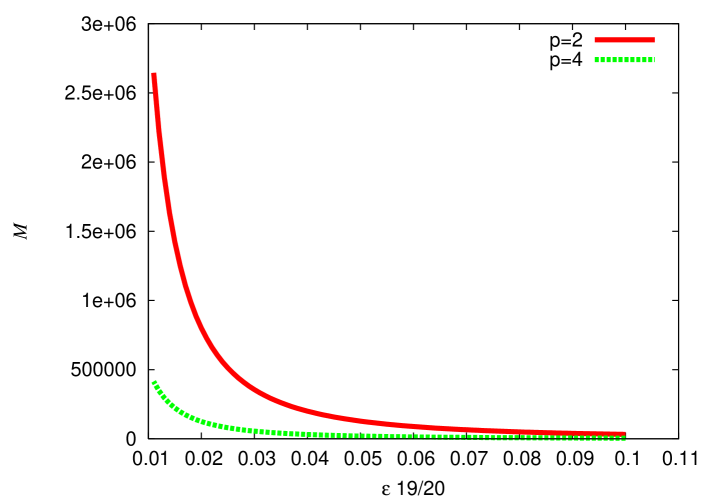
Figure 1: For reliability $1-\delta=0.95$, we plot the memory usage $M$ versus the accuracy $\epsilon$ for pairwise ($p=2$) and 4-wise ($p=4$) independent hash functions as per the bound of Proposition 4. Added independence substantially improves memory requirements for a fixed estimation accuracy according to our theoretical bounds.

Theorem 4.1

Let $X_{1},\ldots,X_{m}$ be a sequence of $p$-wise independent random variables that satisfy $|X_{i}-E(X_{i})|\leq 1$. Let $X=\sum_{i}X_{i}$, then for $C=\max(p,\sigma^{2}(X))$, we have

$$P(|X-\bar{X}|\geq T)\leq\left(\frac{pC}{e^{2/3}T^{2}}\right)^{p/2}.$$

In particular, when $p=2$, we have

$$P(|X-\bar{X}|\geq T)\leq\frac{2C}{e^{2/3}T^{2}}.$$

Proof:

See Schmidt, Siegel, and Srinivasan, Theorem 2.4, Equation III [SSS93]. $\Box$

The following proposition is stated for $n$-grams, but applies generally to arbitrary items.

Proposition 4

Hashing each $n$-gram only once, we can estimate the number of distinct $n$-grams within relative precision $\epsilon$, with a $p$-wise independent hash for $p\geq 2$ by storing $M$ distinct $n$-grams ($M\geq 8p$) and with reliability $1-\delta$ where $\delta$ is given by

$$\delta=\frac{p^{p/2}}{e^{p/3}M^{p/2}}\left(2^{p/2}+\frac{8^{p/2}}{\epsilon^{p}(2^{p/2}-1)}\right).$$

More generally, we have

$$\delta \leq \frac{p^{\frac{p}{2}}}{e^{\frac{p}{3}}M^{\frac{p}{2}}}\left(\frac{\alpha^{\frac{p}{2}}}{(1-\alpha)^{p}}+\frac{4^{\frac{p}{2}}}{\alpha^{\frac{p}{2}}\epsilon^{p}(2^{\frac{p}{2}}-1)}\right).$$

for $4p/M\leq\alpha<1$ and any $p,M$.

Proof:

We generalize a proof by Bar-Yossef et al. [BYJK⁺02] Let $X_{t}$ be the number of distinct elements having only zeros in the first $t$ bits of their hash value. Then $X_{0}$ is the number of distinct elements ($X_{0}=m$). For $j=1,\ldots,m$, let $X_{t,j}$ be the binary random variable with value 1 if the $j^{\textrm{th}}$ distinct element has only zeros in the first $t$ bits of its hash value, and zero otherwise. We have that $X_{t}=\sum_{j=1}^{m}X_{t,j}$ and so $E(X_{t})=\sum_{j=1}^{m}E(X_{t,j})$. Since the hash function is uniform, then $P(X_{t,j}=1)=1/2^{t}$ and so $E(X_{t,j})=1/2^{t}$, and hence, $E(X_{t})=m/2^{t}\Rightarrow 2^{t}E(X_{t})=m$. Therefore $X_{t}$ can be used to determine $m$.

Using pairwise independence, we can can show that $\sigma^{2}(X_{t})\leq\frac{m}{2^{t}}$. We have that $\sigma^{2}(X_{t})\leq\frac{m}{2^{t}}$ because

$$E(|X_{t}-\frac{m}{2^{t}}|^{2}) = E((X_{t}-\frac{m}{2^{t}})^{2})$$

$$= E((\sum_{j=1}^{m}(X_{t,j}-\frac{1}{2^{t}}))^{2})=\sigma^{2}(\sum_{j=1}^{m}X_{t,j})$$

$$= \sum_{j=1}^{m}\sigma^{2}(X_{t,j})\mbox{\ (by $2$-wise independence)}$$

$$= \sum_{j=1}^{m}\frac{1}{2^{t}}(1-\frac{1}{2^{t}})^{2}+(1-\frac{1}{2^{t}})(0-\frac{1}{2^{t}})^{2}$$

$$\leq \sum_{j=1}^{m}\frac{1}{2^{t}}=\frac{m}{2^{t}}.$$

By Theorem 4.1, we have

$$P(|X_{t}-m/2^{t}|\geq\epsilon m/2^{t})\leq\frac{p^{p/2}2^{tp/2}}{m^{p/2}\epsilon^{p}e^{p/3}},\mbox{~{}as long as $\sigma^{2}(X_{t})\geq p$.}$$

Let $M$ be the available memory and suppose that the hash function has $L$ bits such that we know, a priori, that $P(X_{L}>M)\approx 0$. This is necessary since we do not wish to increase $L$ dynamically. It is reasonable since for $L$ and $m$ fixed, $P(X_{L}>M)$ goes down as $1/M^{p}$:

$$P(X_{L}>M) = P(X_{L}-m/2^{L}>M-m/2^{L})$$

$$\leq P(|X_{L}-m/2^{L}|>M-m/2^{L})$$

$$\leq \left(\frac{p\max(m/2^{L},p)}{e^{2/3}(M-m/2^{L})^{2}}\right)^{p/2}$$

for $M-m/2^{L}>0$ where we used Theorem 4.1. For example, if $p=2$, $M=256$, $L=19$, $P(X_{L}>M)\leq 4.4\times 10^{-8}$ for $m=100,000,000$.

The algorithm returns the value $2^{t^{\prime}}X_{t^{\prime}}$ where $t^{\prime}$ is such that $X_{t^{\prime}}\leq M$ and $X_{t^{\prime}-1}>M$. (For a given hash function, note that $X_{i}$ is monotone in $i$ and thus $t^{\prime}$ is uniquely determined by the input and the hash function.) The upshot is that $t^{\prime}$ is itself a random quantity that depends deterministically on the hash function and the input (the same factors that determine $X_{t}$.)

We can bound the error of this estimate as follows.

$$P(|2^{t^{\prime}}X_{t^{\prime}}-m|\geq\epsilon m)$$

$$= \sum_{t=0,\ldots,L}P(|X_{t}-\frac{m}{2^{t}}|\geq\epsilon\frac{m}{2^{t}})P(t^{\prime}=t)$$

$$= \sum_{t=0,\ldots,L}P(|X_{t}-\frac{m}{2^{t}}|\geq\epsilon\frac{m}{2^{t}})P(X_{t-1}>M,X_{t}\leq M).$$

Splitting the summation in two parts, we get

$$P(|2^{t^{\prime}}X_{t^{\prime}}-m|\geq\epsilon m)$$

$$\leq \sum_{t=0}^{\bar{t}-1}P(|X_{t}-\frac{m}{2^{t}}|\geq\epsilon\frac{m}{2^{t}})+\sum_{t=\bar{t},\ldots,L}P(X_{t-1}>M,X_{t}\leq M)$$

$$= P(X_{\bar{t}-1}>M)+\sum_{t=0}^{\bar{t}-1}P(|X_{t}-\frac{m}{2^{t}}|\geq\epsilon\frac{m}{2^{t}})$$

$$\leq P(X_{\bar{t}-1}-m/2^{\bar{t}-1}>M-m/2^{\bar{t}-1})+\sum_{t=0}^{\bar{t}-1}\frac{p^{p/2}2^{tp/2}}{m^{p/2}\epsilon^{p}e^{p/3}}$$

$$\leq P(|X_{\bar{t}-1}-m/2^{\bar{t}-1}|>M-m/2^{\bar{t}-1})+\sum_{t=0}^{\bar{t}-1}\frac{p^{p/2}2^{tp/2}}{m^{p/2}\epsilon^{p}e^{p/3}}$$

$$\leq \left(\frac{pm}{2^{\bar{t}-1}e^{2/3}(M-m/2^{\bar{t}-1})^{2}}\right)^{p/2}+\sum_{t=0}^{\bar{t}-1}\frac{p^{p/2}2^{tp/2}}{m^{p/2}\epsilon^{p}e^{p/3}}$$

$$\leq \frac{p^{p/2}m^{p/2}}{2^{(\bar{t}-1)p/2}e^{p/3}(M-m/2^{\bar{t}-1})^{p}}+\frac{p^{p/2}(2^{{\bar{t}}p/2}-1)}{m^{p/2}\epsilon^{p}e^{p/3}(2^{p/2}-1)}$$

where we assumed that $p\leq m/2^{\bar{t}-1}.$

Choose $\bar{t}\in\{0,\ldots,L\}$ such that $\alpha M/4<\frac{m}{2^{\bar{t}}}\leq\alpha M/2$ for some $\alpha<1$ satisfying $\alpha M/4\geq p$ then

$$\frac{p^{p/2}m^{p/2}}{2^{(\bar{t}-1)p/2}e^{p/3}(M-m/2^{\bar{t}-1})^{p}}\leq\frac{p^{p/2}M^{p/2}\alpha^{p/2}}{e^{p/3}(1-\alpha)^{p}M^{p}}$$

whereas

$$\frac{p^{p/2}(2^{{\bar{t}}p/2}-1)}{m^{p/2}\epsilon^{p}e^{p/3}(2^{p/2}-1)}\leq\frac{p^{p/2}4^{p/2}}{\epsilon^{p}\alpha^{p/2}M^{p/2}e^{p/3}(2^{p/2}-1)}.$$

Hence, we have

$$P(|2^{t^{\prime}}X_{t^{\prime}}-m|\geq\epsilon m) \leq \frac{p^{\frac{p}{2}}}{e^{\frac{p}{3}}M^{\frac{p}{2}}}(\frac{\alpha^{\frac{p}{2}}}{(1-\alpha)^{p}}+\frac{4^{\frac{p}{2}}}{\alpha^{\frac{p}{2}}\epsilon^{p}(2^{\frac{p}{2}}-1)}).$$

Setting $\alpha=1/2$, we have

$$P(|2^{t^{\prime}}X_{t^{\prime}}-m|\geq\epsilon m) \leq \frac{p^{p/2}2^{p/2}}{e^{p/3}M^{p/2}}+\frac{p^{p/2}8^{p/2}}{\epsilon^{p}M^{p/2}e^{p/3}(2^{p/2}-1)}.$$

For different values of $p$ and $\epsilon$, other values of $\alpha$ can give tighter bounds: the best value of $\alpha$ can be estimated numerically. The proof is completed.   $\Box$

It may seem that the result of Proposition 4 is independent of the size of the data set and of the number of distinct symbols ($m$). Indeed, it provides a fixed accuracy $\epsilon$ for a given memory budget ($M$) irrespective of the data source. However, as the proof shows, the number of bits in the hash values need to grow with $\log m$. This requires additional computational costs.

Again the following corollary applies not only to $n$-grams but also to arbitrary items. It follows from setting $M=576/\epsilon^{2}$, $p=2$, and $\alpha=1-\epsilon$.

Corollary 1

With $M=576/\epsilon^{2}$ and $p=2$, we can estimate the count of distinct $n$-grams with reliability ($1-\delta$) of 99% for any $\epsilon>0$.

Proof:

From Proposition 4, consider

$$\delta \leq \frac{p^{\frac{p}{2}}}{e^{\frac{p}{3}}M^{\frac{p}{2}}}\left(\frac{\alpha^{\frac{p}{2}}}{(1-\alpha)^{p}}+\frac{4^{\frac{p}{2}}}{\alpha^{\frac{p}{2}}\epsilon^{p}(2^{\frac{p}{2}}-1)}\right)$$

for $\alpha=1-\epsilon$, $M=576/\epsilon^{2}$, and $p=2$, then

$$\delta \leq \frac{2\epsilon^{2}}{e^{\frac{2}{3}}576}\left(\frac{1-\epsilon}{\epsilon^{2}}+\frac{4}{(1-\epsilon)\epsilon^{2}}\right)$$

$$\leq \frac{2}{e^{\frac{2}{3}}576}\left(1-\epsilon+\frac{4}{(1-\epsilon)}\right).$$

Taking the limit as $\epsilon$ tends to 0, on the basis that the probability of a miss ($P(|X_{t}-m/2^{t}|\geq\epsilon m/2^{t})$) can only grow as $\epsilon$ diminishes, we have that $\delta$ is bounded by ${10}/({e^{\frac{2}{3}}576})\approx 0.008$. $\Box$

This significantly improves the bound of 1/6 for $\delta$ given in Bar-Yossef et al. [BYJK⁺02], for the same value of $M$.

Because $p$-wise independence implies $p-1$-wise independence, memory usage, accuracy and reliability can only improve as $p$ increases. For $p$ large ($p\gg 4$), the result of Proposition 4 is no longer useful because of the $p^{p}$ factor. Other inequalities on $P(|X-\mu|)$ for $p$-wise independent $X$’s should be used.

4.1 Entropy and Iceberg Estimation

With only minor modifications, the techniques used for counting can be modified to provide estimates of various other statistics. We consider entropy [GMV06, CBM06, BDKR02] and iceberg counts [FSGM⁺98]: the GT algorithm is modified to track not only the existence of items hashing to zero, but also the required properties (occurrence counts, for instance) of these items. From this, the statistic can be estimated for the entire data stream.

Let $I$ be the entire set of $n$-grams ($N=\textrm{card}(I)$) and $I^{\prime}$ be the set of probed $n$-grams with $m^{\prime}=\textrm{card}(I^{\prime})$ ($m^{\prime}\in[M/2,M)$). For $i\in I^{\prime}$, we know the exact number of occurrences $f_{i}$ of $i$ and so the probability that any given $n$-gram in $I$ is $i$, $P(i)$, is given by $P(i)=f_{i}/N$. Hence, we can compute $\sum_{i\in I^{\prime}}P(i)\log P(i)$ exactly. A practical one-pass estimate of the Shannon entropy of the $n$-grams ($\sum_{i\in I}P(i)\log P(i)$) is $m/m^{\prime}\sum_{i\in I^{\prime}}P(i)\log P(i)$ since we have a tight estimate for $m$. Unfortunately, we do not have any theoretical results on this estimator. If we were to allow two passes over the data, an unassuming algorithm can estimate the entropy with theoretical bounds [GMV06]. It first samples and then probes.

Various “iceberg count” properties can be handled similarly. In these problems, one is given a predicate on the number of occurrences $f_{i}$ of an item $i$. We seek to estimate the number of distinct items satisfying the predicate. For example, if the predicate is “$f_{i}>c$ for some fixed $c$”, then we wish to estimate $\textrm{card}(\{i\in I|f_{i}>c\})$. For instance, the input text aabaabb contains the 2-grams aa (with count 2), ab (with count 2), ba (with count 1) and bb (with count 1). If the predicate $Q(i)$ is “item $i$ occurs exactly twice”, then the answer to the iceberg query is 2 (because distinct items aa and ab satisfy $Q(i)$. Considering the predicate “$f_{i}>0$”, the iceberg-count problem generalizes the problem of counting distinct $n$-grams.

While we do not have any theoretical bound on the accuracy of such iceberg estimate, we can still model the problem statistically. If we are picking at random $m^{\prime}$ elements from a population of size $m$ having $r<m$ elements satisfying a predicate, the number of elements satisfying the constraint, $Y$, follows an hypergeometric distribution $Y$ with mean $m^{\prime}r/m$ and with variance $m^{\prime}\frac{r(m-r)(m-m^{\prime})}{m^{2}(m-1)}$. Therefore, by Chebyshev’s inequality, we have that $P(|Y-m^{\prime}r/m|<\epsilon m^{\prime}r/m)\leq\frac{(m-r)(m-m^{\prime})}{\epsilon^{2}m^{\prime}r(m-1)}<\frac{m}{\epsilon^{2}m^{\prime}r}$. Hence, we should allocate roughly $M\approx\frac{20m}{\epsilon^{2}r}$ units of storage to have an accuracy of $\epsilon$, 19 times out of 20. Choosing $m^{\prime}=\frac{200m}{r}$ ensures that the number of interesting items found ($Y$) is larger than $190$, 19 times out of 20. Hence, if an upper bound on $m$ and a non-trivial lower bound on $r$ were known, further theoretical results could be possible.

If $M$ is small and the distribution is biased (e.g. Zipfian), such as is the case with $n$-grams of English text, we expect these entropy and iceberg count estimates to be poor.

4.2 Simultaneous Estimation

The GT approach can also be applied to estimate the number of 1-grams, 2-grams, …$n$-grams in one pass over the data. Initially, one might seek hash families such that if $i$ is a $\beta+1$-gram and $j$ is its $\beta$-gram suffix, then $h(i)$ has zero in its first $t$ bits whenever the hash value $h(j)$ has zero in its first $t$ bits. For example, $h(a)=0\Rightarrow h(ba)=0$. Unfortunately, such a family of hash functions cannot be pairwise independent because if $h(\texttt{ba})=0$ then $h(c\texttt{a})=0$ for any value of $c$. However, a straightforward approach can suffice for simultaneous estimation. Separate buffers ($n$ in total) can be kept for each string length ($1$-gram, $2$-gram, …, $n$-gram), and for simplicity we can assume each buffer is of the same size, $M$.

The straightforward approach works as follows: As each of the $N$ symbols in the stream is processed, we hash the $n$ new $n$-grams of size 1, 2, …, $n$ respectively. If each of the $n$ hashes is recursive, then each can be updated from its previous value in O(1) time. However, we can also use semi-recursive hashes with this approach, because the hash value for a $k$-gram can be updated, in O(1) time, to become the hash value for the associated $k+1$-gram.

In particular, the semi-recursive “$n$-wise” hashing scheme examined before becomes more attractive when simultaneous estimation is attempted.

5 Experimental Results

Experiments are used to assess the accuracy of estimates obtained by several hash functions on some input streams. As well, the experiments demonstrate that the techniques can be efficiently implemented. Our code is written in C++ and is available upon request.

5.1 Test Inputs

One complication is that the theoretical predictions are based on worst-case analysis. There may not be a sequence of symbols realizing these bounds. As a result, our experiments used the $n$-grams from a collection of 11 texts from Project Gutenberg. We also used synthetic data sets generated according to various generalized Zipfian distributions. Since we are analyzing the performance of several randomized algorithms, we ran each algorithm 100+ times on each text. We cannot run tests on inputs as large as would be appropriate for corpus linguistics studies: to complete the entire suite of experiments in reasonable time, we must limit ourselves to texts (for instance, Shakespeare’s First Folio) where one run takes at most a few minutes.

5.2 Accuracy of Estimates

Table 1: Maximum error rates $\epsilon$ 19 times out of 20 for various amounts of memory ($M$) and for $p$-wise independent hash values according to Proposition 4 .

	256	1024	2048	65536	262144	1048576
$p=2$	86.4%	36.8%	24.7%	3.8%	1.8%	0.9%
$p=4$	34.9%	16.1%	11.1%	1.8%	0.9%	0.5%
$p=8$	30.0%	14.1%	9.7%	1.6%	0.8%	0.4%

We have theoretical bounds relating to the error $\epsilon$ observed with a given reliability (typically 19/20), when the hash function is taken from a $p$-wise independent family. (See Table 1.) But how close to this bound do we come when $n$-grams are drawn from a “typical” input for a computational-linguistics study? And do hash functions from highly independent families actually enable more accurate estimates?

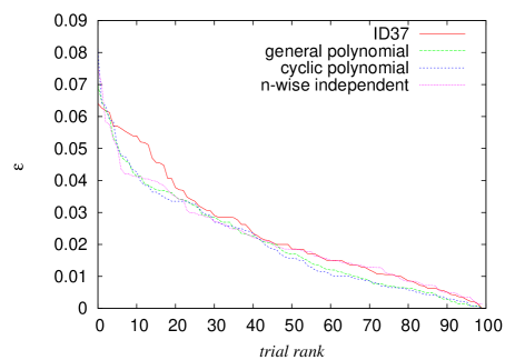
(a) Count estimate errors over Shakespeare’s First Folio (00ws110), 100 runs estimating 10-grams with $M=2048$.

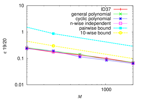
(b) For each $M$ and hash function, worst-case $95^{\textrm{th}}$-percentile error observed on the 11 test inputs

Figure 2: Average relative error $\epsilon$ after 100 runs and over four hash functions.

Figure 2 shows the relative error $\epsilon$ observed from four hash functions (100 estimations with each). Estimates have been ranked by decreasing $\epsilon$, and we see ID37 had more poorer runs than the others. Figure 3 shows a test input (remus10) that was the worst of the 11 for several hash functions, when $M=256$. ID37 seems to be doing reasonably well, but we see $10$-wise independent hashing lagging.

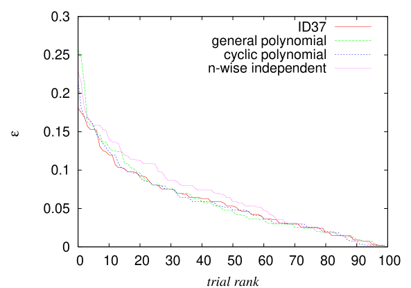
Figure 3: Errors on remus10 (“Uncle Remus His Songs and His Sayings”), from 100 runs estimating 10-grams with $M=256$.

To study the effect of varying $M$, we use the $5^{\textrm{th}}$-largest error of 100 runs. This $95^{\textrm{th}}$-percentile error can be related to the theoretical bound for $\epsilon$ with 19/20 reliability. Figure 2(b) plots the largest $95^{\textrm{th}}$-percentile error observed over 11 test inputs. It is apparent that there is no significant accuracy difference between the hash functions. The $n$-wise independent hash alone has a strong guarantee to be beneath the theoretical bound. However, over the eleven Gutenberg texts, the others are just as accurate, according to our experiments.

5.3 Using a Wider Range of Values for $M$

An important motivation for using $p$-wise independent hashing is to obtain a reliable estimate while only hashing once, using a small $M$. Nevertheless, we have thus far not observed notable differences between the different hash functions. Therefore, although we expect typical values of $M$ to a be few hundred to a few thousand, we can broaden the range of $M$ examined. Although the theoretical guarantees for tiny $M$ are poor, perhaps typical results will be usable. And even a single buffer with $M=2^{20}$ is inconsequential when a desktop computer has several gibibytes of RAM, and the construction of a hash table or B-tree with such a value of $M$ is still quite affordable. Moreover, with a wider range of $M$, we start to see differences between some hash functions.

We choose $M=16$, $16^{2}$, $16^{3}$ and $16^{4}$ and analyze the 5-grams in the text 00ws1 (Shakespeare’s First Folio). There are approximately 300,000 5-grams, and we selected a larger file because when $M=16^{4}$ it seems unhelpful to estimate the number of 5-grams unless the file contains substantially more 5-grams than $M$.

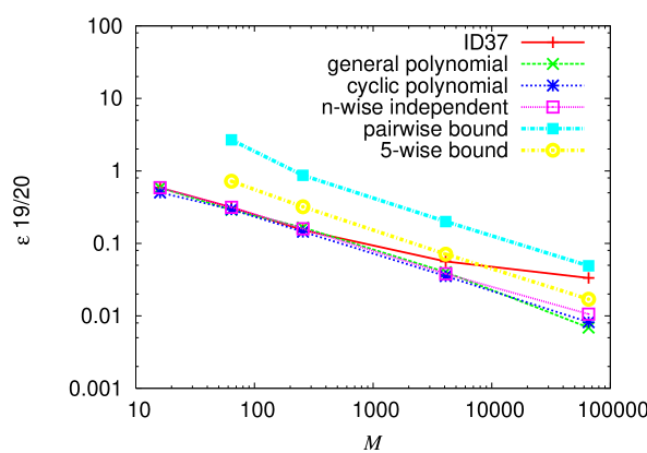
Figure 4: $95^{\textrm{th}}$-percentile error values (for 5-gram estimates) on 00ws1 for various hash families, over a wide range of $M$. Our analysis does not permit prediction of error bounds when $M=16$.

Figure 4 shows the $95^{\textrm{th}}$-percentile errors for Shakespeare’s First Folio, when 5-grams are estimated. There are some smaller differences for $M=65536$ (surprisingly, the $5$-wise hash function, with a better theoretical guarantee, seems to be slightly worse than Cohen’s hash functions). However, it is clear that the theoretical deficiencies in ID37 finally have an effect: it is small when $M=4096$ but clear at $M=65536$. (We observed similar problems on Zipfian data also.) To be fair, this non-uniform hash is still performing better than the pairwise bound, but the trend appears clear. Does it, however, continue for very large $M$?

5.4 Very Large $M$

Clearly, it is only sensible to measure performance when $M\ll m$. Therefore, we estimate the number of $10$-grams obtained when all plain-text files in the Gutenberg CD are concatenated. When $M=2^{20}$, $10$-wise independent hashing had an observed $95^{\textrm{th}}$-percentile error of 0.182% and General had 0.218%. The ID37 error was somewhat worse, at 0.286%. (The theoretical pairwise error bound is 0.908% and the $10$-wise bound is 0.425%. ) Considering the $M=65536$ case from Fig. 4, we see no experimental reason to prefer $n$-wise hashing to General, but ID37 looks less promising. However, $n=10,B=37$ is a non-uniform combination for Integer Division.

5.5 Caveats with Random-Number Generators

To observe the effect of fully independent hashing, we implemented the usual (slow and memory-intensive) scheme where a random value is assigned and stored whenever a key is first seen. Clearly, probabilistic counting of $n$-grams is likely to expose deficiencies in the random-number generator and therefore different techniques were tried. The pseudorandom-number generator in the GNU/Linux C library was tried, as were the Mersenne Twister (MT) [MN98] and also the Marsaglia-Zaman-James (MZJ) generator [MZ87, Jam90, Bou98]. We also tried using a collection of bytes generated from a random physical process (radio static) [Haa98].

For M=4096, the $95^{\textrm{th}}$-percentile error for text 00ws1 was 4.7% for Linux rand(), 4.3% for MT and 4.1% for MZJ. These three pseudorandom number generators were no match for truly random numbers, where the 95% percentile error was only 2.9%. Comparing this final number to Fig. 4, we see fully independent hashing is only a modest improvement on Cohen’s hash functions (which fare better than 5%) despite its stronger theoretical guarantee.

The other hash functions also rely on random-number generation (for $h_{1}$ in Cohen’s hashes and ID37; for $h_{1}\ldots h_{n}$ in the $n$-wise independent hash). It would be problematic if their performance were heavily affected by the precise random-number generation process. However, when we examined the $95^{\textrm{th}}$-percentile errors we did not observe any appreciable differences from varying the pseudorandom-number generation process or using truly random numbers. (The graphs are shown in Appendix A.) Surprisingly, the pseudorandom generators may have been marginally better than the truly random numbers.

5.6 $\textrm{95}^{\textrm{th}}$-Percentile Errors Using Zipfian Data

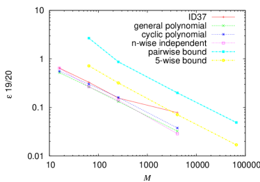
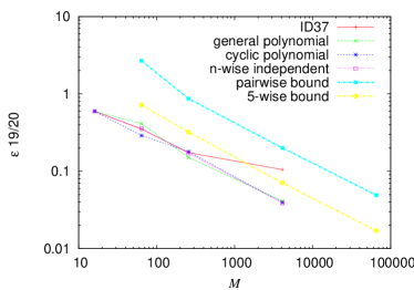
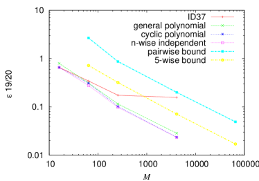
Figure 5: n=5 Zipfian data, $s=1$ (top left), $s=1.2$ (top right), $s=1.6$ (bottom left) and $s=2$ (bottom right).

The various hash functions were also tested on synthetic Zipfian data, where the probability of the $k^{\textrm{th}}$ symbol is proportional to $k^{-s}$. (We chose $s\in[0.8,2.0]$.) Each data set had $N\approx 10^{5}$, but for larger values of $s$ there were significantly fewer $n$-grams. Therefore, measurements for $M$=65536 would not be meaningful and are omitted.

Some results, for $n=5$, are shown in Fig. 5. The ID37 method is noteworthy. Its performance for larger $M$ is badly affected by increasing $s$. The other hash functions are nearly indistinguishable in almost all other cases. Results are similar for 5-grams and 10-grams (which are not shown), except that $s$ can grow slightly bigger for 10-grams before ID37 fails badly.

5.7 Choosing Between Cohen’s Hash Functions

The experiments reported so far do not reveal a clear distinction, at least at the $95^{\textrm{th}}$ percentile error, between Cohen’s General and his Cyclic polynomial hashes. This is somewhat surprising, considering the theoretical differences (nonuniformity versus pairwise independence) shown in Lemma 2 and Lemma 3.

The ratio $m/M$ may be significant (because this ratio affects how many hash bits are used) and our experiments thus cover two different ratios. We first used synthetic Zipfian data ($s=2$), looking for $5$-grams, since that combination revealed the weakness of ID37. Since $m=14826$ for our Zipfian data set, choosing $M=64$ gives a ratio about 231 and $M=1024$ gives a ratio of about 14.

Results, for more than 2000 runs, are shown in Table 2. The top of the table shows $\epsilon$ values (percents), with boldfacing indicating a case when one technique had a lower error than the other. It shows a slightly better performance for Cyclic. Means also slightly favour Cyclic. This is consistent with the experimental results reported by Cohen [Coh97].

Table 2: Comparing polynomial hashes Cyclic and General, Zipfian data set.

percentile	Cyclic		General
	M=64	M=1024	M=64	M=1024
25	3.60	0.931	3.60	0.931
50	7.06	1.98	8.49	2.01
75	14.0	3.41	13.7	3.60
95	30.9	6.11	31.2	6.22
mean	10.6	2.45	10.7	2.51

We also ran more extensive tests using 00ws1, where there seems to be no notable distinction. 10,000 test runs were made. Results are shown in Table 3. The overall conclusion is that the theoretical advantage held by General does not carry over. Experimentally, these two techniques cannot be distinguished meaningfully by our tests.

Table 3: Comparing polynomial hashes Cyclic and General, data set 00ws1

percentile	Cyclic		General
	M=64	M=1024	M=64	M=1024
25	5.79	1.30	5.79	1.30
50	10.7	2.58	10.7	2.69
75	18.2	4.55	19.0	4.55
95	30.6	7.69	30.6	7.69
mean	12.5	3.15	12.6	3.14

5.8 Estimating Iceberg Counts and Entropy

Although we do not have a theoretical bound to compare with, experiments tested the approach to single-pass iceberg-count and entropy estimation given Section 4.1. On our 11 data sets, the amounts of relative error (for 5-grams) observed with a 95% reliability are shown in Figs. 6–7. (The data is shown separately for the 6 data sets with 100,000 or more 5-grams, since the $M=65536$ case is uninteresting for the other 5 data sets.) The iceberg-count estimates the number of distinct $n$-grams occurring at least 10 times.

We see that the error of estimates does decrease quickly with $M$, and that when $M<4096$, the accuracy was poor. However, the accuracy when $M=4096$ might be adequate for some applications.

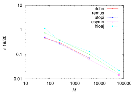
(a) Entropy estimates

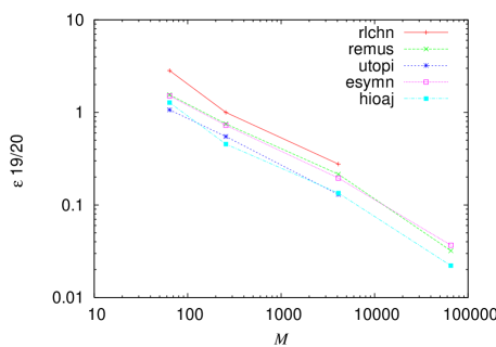
(b) Iceberg-count estimates

Figure 6: Relative errors on smaller data sets: rlchn, remus, utopi, esymn and hioaj. Points with zero error are omitted, due to the logarithmic axes.

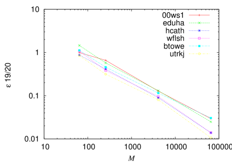
(a) Entropy estimates

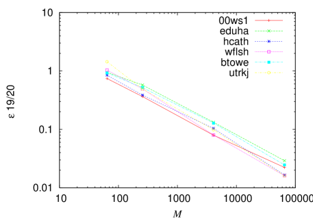
(b) Iceberg-count estimates

Figure 7: Relative errors on larger data sets: 00ws1, eduha, hcath, wflsh, btowe and utrkj.

While we expected poor results on English texts due to the biased distribution, the results suggest that useful theoretical bounds are possible.

5.9 Speed

Speeds were measured on a Dell Power Edge 6400 multiprocessor server (with four Pentium III Xeon 700 MHz processors having 2 MiB cache each, sharing 2 GiB of 133 MHz RAM). The OS kernel was Linux 2.4.20 and the GNU C++ compiler version 3.2.2 was used with relevant compiler flags -O2 -march=i686 -fexceptions. The STL map class was used to construct look-up tables.

Only one processor was used, and the data set consisted of all the plain text files on the Project Gutenberg CD, concatenated into a single disk file containing over 400 MiB and approximately 116 million 10-grams. For comparison, this file was too large to process with the Sary suffix array [Tak05] package (version 1.2.0), since the array would have exceeded 2 GiB. However, the first 200 MB was successfully processed by Sary, which took 1886 s to build the suffix array. The SUFARY [Yam05] (version 2.3.8) package is said to be faster than sary [Tak05]. It processed the 200 MB file in 2640 s and then required 95 s to (exactly) compute the number of 5-grams with more than 100,000 occurrences.

Table 4: Time (seconds) to process all Gutenberg CD files, $10$-grams.

Hashing	$M=2^{10}$	$M=2^{20}$
$10$-wise	794	938
ID37	268	407
Cyclic	345	486
General	352	489

From Table 4 we see that $n$-gram estimation can be efficiently implemented. First, comparing results for $M=2^{20}$ to those for $M=2^{10}$, we see using a larger table costs roughly 140 s in every case. This increase is small when considering that $M$ was multiplied by $2^{10}$ and is consistent with the fact that the computational cost is dominated by the hashing. Comparing different hashes, using a $10$-wise independent hash was about twice as slow as using a recursive hash. Hashing with ID37 was 15–25% faster than using Cohen’s approaches.

Assuming that we are willing to allocate very large files to create suffix arrays and use much internal memory, an exact count is still at least 10 times more expensive than an approximation. Whereas the suffix-array approach would take about an hour to compute $n$-gram counts over the entire Gutenberg CD, an estimate can be available in about 6 minutes while using very little memory and no permanent storage.

6 Conclusion

Considering speed, theoretical guarantees, and actual results, we recommend Cohen’s General. It is fast, has a theoretical performance guarantee, and behaves at least as well as either ID37 or the $n$-wise independent approach. General is pairwise independent so that there are minimal theoretical bounds to its performance. The $n$-wise independent hashing comes with a stronger theoretical guarantee, and thus there can be no unpleasant surprises with its accuracy on any data set. Yet there is a significant speed penalty for its use in our implementation. The speed gain of ID37 is worthwhile only for very small values of $M$. Not only does it lack a theoretical accuracy guarantee, but for larger $M$ it is observed to fall far behind the other hashing approaches in practice. Except where accuracy is far less important than speed, we cannot recommend ID37.

Iceberg-count and entropy estimates on English text showed good decay with larger values of $M$ warranting further theoretical investigations.

There are various avenues for follow-up work that we are pursuing. Further improvements to the theoretical bound seem possible, especially for larger values of $p$. A more sophisticated solution to the simultaneous estimation problem may be possible, and it could be experimentally evaluated against the approach sketched in Section 4.2 and against suffix-array methods.

Efficient frequent string mining have been recently proposed [FHK05] to find frequent substrings in one string that are rare in another. However, suffix arrays do not support fast search for the most frequent phrases containing a given word. While suffix arrays allow us to count occurrences of a substring, they provide no means to count the occurrences of the various $n$-grams beginning with a given substring, let alone the $n$-grams containing a substring.

Appendix A Pseudorandom-Number Generators and Accuracy

The following graphs show that varying the source of random (or pseudorandom) numbers had little effect on General, Cyclic or the $n$-wise random hashes.

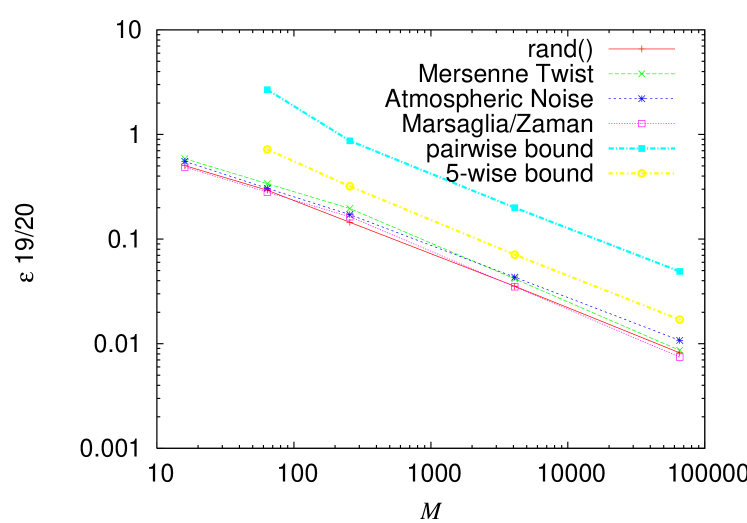
Figure 8: Cyclic is not affected much by the source of random numbers.

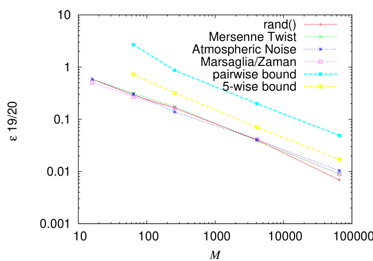
Figure 9: General is similarly unaffected.

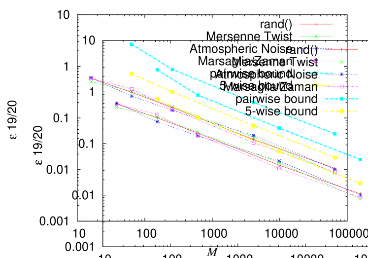
Figure 10: The $n$-wise independent hash is similarly unaffected

References

- [BDKR02] Tugkan Batu, Sanjoy Dasgupta, Ravi Kumar, and Ronitt Rubinfeld. The complexity of approximating entropy. In STOC’02, pages 678–687, New York, NY, USA, 2002. ACM Press.
- [Ber95] Michel Bernard. À juste titre: A lexicometric approach to the study of titles. Literary and Linguistic Computing, 10(2):135–141, 1995.
- [BGKS06] L. Bhuvanagiri, S. Ganguly, D. Kesh, and C. Saha. Simpler algorithm for estimating frequency moments of data streams. SODA’06, pages 708–713, 2006.
- [BH84] Francis L. Bacon and Donald J. Houde. Data compression apparatus and method. US Patent 4612532, 1984. filed 1984; granted 1986. Assignee Telebyte (later Telcor Systems).
- [Bou98] Paul Bourke. Uniform random number generator. online: http://astronomy.swin.edu.au/~pbourke/other/random/index.html, March 1998. checked 2006-06-16.
- [BS05] R. P. Jagadeesh Chandra Bose and S. H. Srinivasan. Data mining approaches to software fault diagnosis. In RIDE ’05, pages 45–52, Washington, DC, USA, 2005. IEEE Computer Society.
- [BWZ02] Dirk Bahle, Hugh E. Williams, and Justin Zobel. Efficient phrase querying with an auxiliary index. In SIGIR ’02: Proceedings of the 25th annual international ACM SIGIR conference on Research and development in information retrieval, pages 215–221, New York, NY, USA, 2002. ACM Press.
- [BYJK+02] Ziv Bar-Yossef, T. S. Jayram, Ravi Kumar, D. Sivakumar, and Luca Trevisan. Counting distinct elements in a data stream. In RANDOM’02, pages 1–10, 2002.
- [Can06] John Canny. CS174 lecture notes. http://www.cs.berkeley.edu/~jfc/cs174/lecs/lec10/lec10.pdf, 2006. checked 2006-06-01.
- [CBM06] Amit Chakrabarti, Khanh Do Ba, and S. Muthukrishnan. Estimating entropy and entropy norm on data streams. In STACS 2006, 2006.
- [CGR01] Paolo Ciaccia, Matteo Golfarelli, and Stefano Rizzi. On estimating the cardinality of aggregate views. In DMDW, pages 12.1–12.10, 2001.
- [CGR03] P. Ciaccia, M. Golfarelli, and S. Rizzi. Bounding the cardinality of aggregate views through domain-derived constraints. Data & Knowledge Engineering, 45(2):131–153, 2003.
- [CHA02] P. Cohen, B. Heeringa, and N. Adams. Unsupervised segmentation of categorical time series into episodes. In ICDM’02, pages 99–106, 2002.
- [CMS01] Maria Fernanda Caropreso, Stan Matwin, and Fabrizio Sebastiani. A learner-independent evaluation of the usefulness of statistical phrases for automated text categorization, pages 78–102. Idea Group Publishing, Hershey, PA, USA, 2001.
- [Cod93] E.F. Codd. Providing OLAP (on-line analytical processing) to user-analysis: an IT mandate. Technical report, E.F. Codd and Associates, 1993.
- [Coh97] Jonathan D. Cohen. Recursive hashing functions for n-grams. ACM Trans. Inf. Syst., 15(3):291–320, 1997.
- [CP06] M. Chang and C.K. Poon. Efficient phrase querying with common phrase indexing. In ECIR’06, 2006.
- [CW79] L. Carter and M.N. Wegman. Universal classes of hash functions. Journal of Computer and System Sciences, 18(2):143–154, 1979.
- [DERC06] F.B. Dehne, T.B. Eavis, and A.B. Rau-Chaplin. The cgmCUBE project: Optimizing parallel data cube generation for ROLAP. Distributed and Parallel Databases, 19(1):29–62, 2006.
- [DF03] M. Durand and P. Flajolet. Loglog counting of large cardinalities. In European Symposium on Algorithms. Springer, 2003.
- [DK04] M. Deshpande and G. Karypis. Selective Markov models for predicting web page accesses. ACM Transactions on Internet Technology (TOIT), 4(2):163–184, 2004.
- [DMKS05] R. Dementiev, J. Mehnert, J. Karkkainen, and P. Sanders. Better external memory suffix array construction. In ALENEX05: Workshop on Algorithm Engineering & Experiments, 2005.
- [DR03] S. Doraisamy and S. Rüger. Position indexing of adjacent and concurrent n-grams for polyphonic music retrieval. In ISMIR 2003, pages 227–228, 2003.
- [Dro03] M. Droettboom. Correcting broken characters in the recognition of historical printed documents. In Digital Libraries 2003, pages 364–366, 2003.
- [FB06] Alex Franz and Thorsten Brants. All our n-gram are belong to you. in the Google Research Blog, http://googleresearch.blogspot.com/2006/08/, March 2006. checked 2006-08-09.
- [FHK05] Johannes Fischer, Volker Heun, and Stefan Kramer. Fast frequent string mining using suffix arrays. In ICDM’05, 2005.
- [FM85] P. Flajolet and G.N. Martin. Probabilistic counting algorithms for data base applications. Journal of Computer and System Sciences, 31(2):182–209, 1985.
- [FMS96] C. Faloutsos, Y. Matias, and A. Silberschatz. Modeling skewed distribution using multifractals and the 80-20 law. In VLDB’96, pages 307–317, 1996.
- [FSGM+98] Min Fang, Narayanan Shivakumar, Hector Garcia-Molina, Rajeev Motwani, and Jeffrey D. Ullman. Computing iceberg queries efficiently. In VLDB’98, pages 299–310, San Francisco, CA, USA, 1998. Morgan Kaufmann Publishers Inc.
- [GBLP96] J. Gray, A. Bosworth, A. Layman, and H. Pirahesh. Data cube: A relational aggregation operator generalizing group-by, cross-tab, and sub-total. In ICDE ’96, pages 152–159, 1996.
- [GBY90] G. H. Gonnet and R. A. Baeza-Yates. An analysis of the Karp-Rabin string matching algorithm. Information Processing Letters, 34(5):271–274, 1990.
- [GKS99] R. Giegerich, S. Kurtz, and J. Stoye. Efficient implementation of lazy suffix trees. In WAE’99, pages 30–42, 1999.
- [GMV06] Sudipto Guha, Andrew McGregor, and Suresh Venkatasubramanian. Streaming and sublinear approximation of entropy and information distances. In SODA’06, pages 733–742, New York, NY, USA, 2006. ACM Press.
- [GT01] Phillip B. Gibbons and Srikanta Tirthapura. Estimating simple functions on the union of data streams. In SPAA’01, pages 281–291, 2001.
- [GZ01] Jianfeng Gao and Min Zhang. Improving language model size reduction using better pruning criteria. In ACL’02: Proceedings of the 40th Annual Meeting on Association for Computational Linguistics, pages 176–182, Morristown, NJ, USA, 2001. Association for Computational Linguistics.
- [Haa98] Mads Haahr. random.org — true random number service. online, http://www.random.org, October 1998. checked 2006-06-16.
- [HNSS95] P.J. Haas, J.F. Naughton, S. Seshadri, and L. Stokes. Sampling-based estimation of the number of distinct values of an attribute. In VLDB’95, pages 311–322, 1995.
- [HSS03] W.K. Hon, K. Sadakane, and W.K. Sung. Breaking a time-and-space barrier in constructing full-text indices. In FOCS’03, pages 251–260, 2003.
- [IW05] P. Indyk and D. Woodruff. Optimal approximations of the frequency moments of data streams. Proceedings of the thirty-seventh annual ACM symposium on Theory of computing, pages 202–208, 2005.
- [Jam90] F. James. A review of pseudorandom number generators. Computer Physics Communications, 60:329–344, 1990.
- [Jel98] F. Jelinek. Statistical methods for speech recognition. MIT Press Cambridge, MA, USA, 1998.
- [JSB06] Patrick Joula, John Sofko, and Patrick Brennan. A prototype for authorship attribution studies. Literary and Linguistic Computing, 21(2):169–178, 2006.
- [KC04] V. Keselj and N. Cercone. CNG method with weighted voting. In P. Joula, editor, ad-hoc Authorship Attribution Contest. AHC/ALLC, 2004.
- [KKL05a] Steven Keith, Owen Kaser, and Daniel Lemire. Analyzing large collections of electronic text using OLAP. In APICS 2005, October 2005.
- [KKL05b] Steven Keith, Owen Kaser, and Daniel Lemire. Analyzing large collections of electronic text using OLAP. Technical Report TR-05-001, UNBSJ CSAS, June 2005.
- [KMR+94] Michael Kearns, Yishay Mansour, Dana Ron, Ronitt Rubinfeld, Robert E. Schapire, and Linda Sellie. On the learnability of discrete distributions. In STOC’94, pages 273–282, 1994.
- [Knu69] Donald E. Knuth. Seminumerical Algorithms, volume 2 of The Art of Computer Programming. Addison-Wesley, 1969.
- [Kot02] Yannis Kotidis. Handbook of Massive Data Sets, chapter Aggregate View Management in Data Warehouses, pages 711–741. Kluwer Academic Publishers, Norwell, MA, USA, 2002.
- [KR87] R.M. Karp and M.O. Rabin. Efficient randomized pattern-matching algorithms. IBM Journal of Research and Development, 31(2):249–260, 1987.
- [KW98] C. Kit and Y. Wilks. The Virtual Corpus approach to deriving n-gram statistics from large scale corpora. In Proceedings of 1998 International Conference on Chinese Information Processing, pages 223–229, 1998.
- [KW06] M. Kolonko and D. Wasch. Sequential reservoir sampling with a nonuniform distribution. ACM Trans. Math. Softw., 32(2):257–273, 2006.
- [KWLL05] Min-Soo Kim, Kyu-Young Whang, Jae-Gil Lee, and Min-Jae Lee. n-gram/2l: a space and time efficient two-level n-gram inverted index structure. In VLDB’05, pages 325–336. VLDB Endowment, 2005.
- [LH03] Chin-Yew Lin and Eduard Hovy. Automatic evaluation of summaries using n-gram co-occurrence statistics. In NAACL’03, pages 71–78, Morristown, NJ, USA, 2003. Association for Computational Linguistics.
- [Li94] Kim-Hung Li. Reservoir-sampling algorithms of time complexity O(n(1 + log(N/n))). ACM Trans. Math. Softw., 20(4):481–493, 1994.
- [LK06] Daniel Lemire and Owen Kaser. One-pass, one-hash -gram count estimation. Under review, 2006.
- [LOK00] Paul Losiewicz, Douglas W. Oard, and Ronald N. Kostoff. Textual data mining to support science and technology management. J. Intell. Inf. Syst., 15(2):99–119, 2000.
- [MCDA03] Josiane Mothe, Claude Chrisment, Bernard Dousset, and Joel Alaux. DocCube: Multi-dimensional visualization and exploration of large document sets. Journal of the American Society for Information Science and Technology, 54(7):650–659, 2003.
- [MLC+00] M. C. McCabe, J. Lee, A. Chowdhury, D. Grossman, and O. Frieder. On the design and evaluation of a multi-dimensional approach to information retrieval. In SIGIR ’00, pages 363–365, New York, NY, USA, 2000. ACM Press.
- [MM90] Udi Manber and Gene Myers. Suffix arrays: a new method for on-line string searches. In SODA ’90, pages 319–327, Philadelphia, PA, USA, 1990. Society for Industrial and Applied Mathematics.
- [MM93] Udi Manber and Gene Myers. Suffix arrays: a new method for on-line string searches. SIAM Journal on Computing, 22(5):935–948, 1993.
- [MN98] M. Matsumoto and T. Nishimura. Mersenne Twister: A 623-dimensionally equidistributed uniform pseudo-random number generator. ACM Transactions on Modeling and Computer Simulation, 8(1):3–30, 1998.
- [MS00] David A. McAllester and Robert E. Schapire. On the convergence rate of Good-Turing estimators. In COLT’00: Proceedings of the Thirteenth Annual Conference on Computational Learning Theory, pages 1–6, San Francisco, CA, USA, 2000. Morgan Kaufmann Publishers Inc.
- [MZ87] George Marsaglia and Arif Zaman. Toward a universal random number generator. Technical Report FSU-SCRI-87-50, Florida State University, 1987.
- [NGZZ00] Jian-Yun Nie, Jiangfeng Gao, Jian Zhang, and Ming Zhou. On the use of words and n-grams for Chinese information retrieval. In IRAL’00: Proceedings of the Fifth International Workshop on on Information Retrieval with Asian Languages, pages 141–148, New York, NY, USA, 2000. ACM Press.
- [NHJ03] Timo Niemi, Lasse Hirvonen, and Kalerva Järvelin. Multidimensional data model and query language for informetrics. Journal of the American Society for Information Science and Technology, 54(10):939–951, 2003.
- [NM94] Makoto Nagao and Shinsuke Mori. A new method of n-gram statistics for large number of n and automatic extraction of words and phrases from large text data of Japanese. In COLING’94, pages 611–615, 1994.
- [NT03] T.P.E. Nadeau and T.J.E. Teorey. A Pareto model for OLAP view size estimation. Information Systems Frontiers, 5(2):137–147, 2003.
- [OSZ03] A. Orlitsky, NP Santhanam, and J. Zhang. Always Good Turing: asymptotically optimal probability estimation. In FOCS’03, pages 179–188, 2003.
- [PK03] JK Paulus and AP Klapuri. Conventional and periodic n-grams in the transcription of drum sequences. In ICME’03, pages 737–740, 2003.
- [Pro06] Project Gutenberg Literary Archive Foundation. Project Gutenberg. http://www.gutenberg.org/, 2006. checked 2006-10-17.
- [Rus06] Frank Ruskey. The (combinatorial) object server. http://www.theory.cs.uvic.ca/~cos/cos.html, 2006. checked 2006-06-01.
- [SDNR96] A. Shukla, P. Deshpande, J.F. Naughton, and K. Ramasamy. Storage estimation for multidimensional aggregates in the presence of hierarchies. In VLDB’96, pages 522–531, 1996.
- [Sha48] Claude E. Shannon. A mathematical theory of communications. Bell Syst. Tech. J, 1948.
- [Sie89] A. Siegel. On universal classes of fast high performance hash functions, their time-space tradeoff, and their applications. In FOCS’89, pages 20–25, 1989.
- [SRR04] B. Shah, K. Ramachandran, and V. Raghavan. Storage estimation of multidimensional aggregates in a data warehouse environment. In Proceedings of the World Multi-Conference on Systemics, Cybernetics and Informatics, 2004.
- [SSS93] J.P. Schmidt, A. Siegel, and A. Srinivasan. Chernoff-Hoeffding bounds for applications with limited independence. In SODA’93, pages 331–340. Society for Industrial and Applied Mathematics Philadelphia, PA, USA, 1993.
- [Sul01] D. Sullivan. Document Warehousing and Text Mining: Techniques for Improving Business Operations, Marketing, and Sales. John Wiley & Sons, 2001.
- [Sun04] Sun Microsystems. String (Java 2 Platform SE 5.0). online documentation: http://java.sun.com/j2se/1.5.0/docs/api/index.html, 2004.
- [SYLZ00] Z. Su, Q. Yang, Y. Lu, and H. Zhang. WhatNext: a prediction system for web requests using n-gram sequence models. In Web Information Systems Engineering 2000, pages 214–221, 2000.
- [Tak05] Satoru Takabayashi. Sary: A suffix array library and tools. online: http://sary.sourceforge.net/, March 2005. checked 2006-06-28.
- [Vit85] Jeffrey S. Vitter. Random sampling with a reservoir. ACM Trans. Math. Softw., 11(1):37–57, 1985.
- [Wei99] M. Weiss. Data Structures and Algorithm Analysis in Java. Addison Wesley, 1999.
- [WVZT90] K.Y.U.Y. Whang, B.T. Vander-Zanden, and H.M. Taylor. A linear-time probabilistic counting algorithm for database applications. ACM Transactions on Database Systems, 15(2):208–229, 1990.
- [Yam05] Tatsuo Yamashita. SUFARY. online: http://nais.to/~yto/tools/sufary, January 2005. checked 2006-06-28.
- [YTH90] E. J. Yannakoudakis, I. Tsomokos, and P. J. Hutton. n-Grams and their implication to natural language understanding. Pattern Recogn., 23(5):509–528, 1990.
- [YZS05] Xiaohui Yu, Calisto Zuzarte, and Kenneth C. Sevcik. Towards estimating the number of distinct value combinations for a set of attributes. In CIKM’05: Proceedings of the 14th ACM International Conference on Information and Knowledge Management, pages 656–663, New York, NY, USA, 2005. ACM Press.
- [ZMR98] J. Zobel, A. Moffat, and K. Ramamohanarao. Inverted files versus signature files for text indexing. ACM Transactions on Database Systems, 23(4):453–490, 1998.