Detection of Markov Random Fields on Two-Dimensional Intersymbol Interference Channels

Abstract

We present a novel iterative algorithm for detection of binary Markov random fields (MRFs) corrupted by two-dimensional (2D) intersymbol interference (ISI) and additive white Gaussian noise (AWGN). We assume a first-order binary MRF as a simple model for correlated images. We assume a 2D digital storage channel, where the MRF is interleaved before being written and then read by a 2D transducer; such channels occur in recently proposed optical disk storage systems. The detection algorithm is a concatenation of two soft-input/soft-output (SISO) detectors: an iterative row-column soft-decision feedback (IRCSDF) ISI detector, and a MRF detector. The MRF detector is a SISO version of the stochastic relaxation algorithm by Geman and Geman in IEEE Trans. Pattern Anal. and Mach. Intell., Nov. 1984. On the $2\times 2$ averaging-mask ISI channel, at a bit error rate (BER) of $10^{-5}$, the concatenated algorithm achieves SNR savings of between 0.5 and 2.0 dB over the IRCSDF detector alone; the savings increase as the MRFs become more correlated, or as the SNR decreases. The algorithm is also fairly robust to mismatches between the assumed and actual MRF parameters.

I Introduction

This paper considers the detection of an $M\times N$ binary-valued 2D MRF $F$ transmitted over the digital storage channel shown in Fig. 1. The received image

$$r(m,n)=\sum_{k}\sum_{l}h(k,l)\tilde{F}(m-k,n-l)+w(m,n),$$ (1)

where $0\leq m\leq M-1$, $0\leq n\leq N-1$, $h(k,l)$ is a finite-impulse-response 2D blurring mask, $\tilde{F}=2\times\pi(F)-1$ is an interleaved and level-shifted version of $F$, the $w(m,n)$ are zero mean i.i.d. Gaussian random variables (r.v.s) with variance $\sigma_{w}^{2}$, and the double sum is computed over the mask support region $\mbox{$\mathcal{S}$}_{h}=\{(k,l):h(k,l)\neq 0\}$. The MRF $F$ takes pixel values from $\{0,1\}$, and is correlated according to the following Markov property [1]:

$$\begin{split}\mathrm{Pr}(F_{m,n}=f_{m,n}|F_{k,l}=f_{k,l},(k,l)\neq(m,n))\\ =\mathrm{Pr}(F_{m,n}=f_{m,n}|F_{k,l}=f_{k,l},(k,l)\in\mathcal{F}_{m,n}).\end{split}$$ (2)

In (2), $F_{m,n}$ denotes pixel $(m,n)$ of the MRF, $f_{k,l}$ denotes a particular value of pixel $(k,l)$, and $\mathcal{F}_{m,n}$ denotes the first-order neighborhood of pixel $(m,n)$: $\mathcal{F}_{m,n}=\{(m,n-1),(m,n+1),(m-1,n),(m+1,n)\}$. The MRF $F$ is generated by a Gibbs sampler based on the Ising model, which is characterized by a two parameter energy function. It is assumed that the detector knows the energy parameters (and therefore the complete Markov model) of the transmitted MRF. Because of the interleaver, it is assumed that the pixels in $\tilde{F}$ are independent and identically distributed (i.i.d.), with $\mathrm{Pr}\{F(m,n)=0\}=p_{0}=1-p_{1}$ for all $(m,n)$, where the a priori probabilities $p_{0}$ and $p_{1}$ need not in general equal $1/2$.

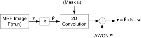
Figure 1: Block diagram of the digital storage channel assumed in this paper; the $\pi$ represents an image interleaver, and $*$ represents 2D convolution. Level shifting from $\{0,1\}$ to $\{-1,1\}$, performed after the interleaver, is not shown.

The motivating application for the channel model employed in this paper is 2D magnetic or optical storage systems, which are subject to 2D ISI. Such systems (e.g., [2]) store the image $\tilde{F}$ in its original 2D form, rather than converting the image to a 1D sequence and storing it on 1D tracks. Over the past 10 years, a number of papers (e.g., [3]-[14]) have considered the detection problem for binary images on the 2D ISI channel, under the assumption that the transmitted image pixels are i.i.d. and equiprobable. In practice, this i.i.d. assumption can be largely achieved by interleaving the original image before storage (as in Fig. 1), and deinterleaving it after detection. However, in practice the original image is often correlated. Uncompressed natural images are highly correlated; these typically occur in diagnostic medical imaging where distortion due to lossy compression is intolerable, and the time required for lossless compression/decompression may not be available. Images usually retain some correlation even if stored in compressed format, because practical lossless (or lossy) image compression schemes do not completely decorrelate the image.

The principal contribution of the present paper is an iterative detection scheme that exploits the correlation in the original image to achieve significant SNR savings over ISI detection schemes which do not account for correlated input images. Although we model the image correlation by a simple first-order Markov random field, our results give at least a proof of principle that can be further explored with more realistic image models. A key innovation introduced in this paper is a soft-input, soft-output MRF detection algorithm, based on the stochastic relaxation image restoration algorithm of [1]. The ISI detector employed in this paper is described in [12, 14], where comparisons with several previously published algorithms show that it is among the best performing ISI detectors in the public domain.

II The Concatenated Detector

A block diagram of the concatenated system is shown in Fig. 2. It operates according to the “turbo principle” (after turbo-codes [15]), whereby two or more SISO decoders exchange extrinsic information and iterate until convergence. The received image $\mathbf{r}$ is an input to the ISI detector, which attempts to remove the ISI under the assumption that the pixels of $\tilde{F}$ are i.i.d. The ISI detector outputs deinterleaved extrinsic log-likelihood ratios (LLRs) to the MRF detector, which estimates the original MRF $F$, and feeds back interleaved extrinsic LLRs to the ISI detector.

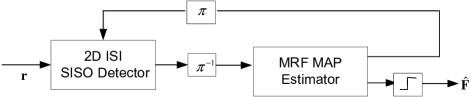
Figure 2: Block diagram of the concatenated detector.

II-A The ISI Detector

A detailed description of the ISI detector, including performance comparisons with a number of other previously published 2D ISI algorithms, appears in [12, 14]. The ISI detector is therefore only briefly described here.

Figure 3: ISI detector block diagram. The extrinsic input from the MRF detector into the row-SISO is not shown.

Figure 3 is a block diagram of the ISI detector, which employs an iterative, row-column soft-decision feedback algorithm (IRCSDFA). The IRCSDFA consists of two SISO modules, run on rows and columns, which exchange weighted soft information estimates of the interleaved MRF $\tilde{F}$. Each module runs the BCJR algorithm [16] on several rows (columns) of the image at once, and uses soft decision feedback from previously-processed rows (columns), to arrive at an LLR estimate $\tilde{L}$ of the current row (or column.) The weight $w$ attenuates the LLR estimates, to correct for the over-confidence effect resulting from use of soft decision feedback (SDF).

The row-SISO trellis state and input block for the $m$th row of an image corrupted by $2\times 2$ ISI is shown in Fig. 4. A trellis is generated by shifting this block right one column at a time through all the pixels in a given row, and taking into account the eight possible values of the three input pixels. The resulting trellis has eight states and eight branches per state. Each trellis branch metric is the sum of three terms; each term is the squared Euclidean distance (SED) between one of the 2D inner products shown in Fig. 4 and the corresponding received pixel $r(m,n)$, $r(m+1,n)$, or $r(m+2,n)$. Each 2D inner product is computed between the inverted convolution mask $h(m-k,n-l)$ and the appropriate block of state, input, and feedback pixels indicated in Fig. 4; to compute inner product 2 shown in the figure, the inverted mask’s $h(0,0)$ coefficient overlays the current pixel position $(m,n)$. The algorithm uses the LLRs $\omega_{1}$ and $\omega_{2}$ from the previously processed row as soft-decision feedback when computing modified pixel transition probabilities $\gamma_{\mathbf{i}}(\mathbf{r}_{k},s^{\prime},s)$ in the BCJR algorithm, where $\mathbf{i}=[i_{0},i_{1},i_{2}]$ and $\mathbf{r}=[r(m,n),r(m+1,n),r(m+2,n)]$ denote input and received pixel vectors (as seen in Fig. 4), $k$ denotes the iteration number, and the candidate input pixels $i_{j}$ take values from $\{-1,1\}$ with a priori probabilities $p_{0}$ and $p_{1}$.

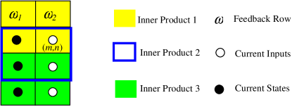
Figure 4: The ISI detector’s row-SISO trellis states and inputs, for a $2\times 2$ mask.

The modified $\gamma$ is the product of a modified conditional channel PDF $p^{\prime}(\cdot)$ (which takes into account the SDF LLRS $\omega_{1}$ and $\omega_{2}$, and which is described further in [12, 14]), trellis transition probabilities, and extrinsic information from the other decoder:

$$\begin{split}&\gamma_{\mathbf{i}}(\mathbf{r}_{k},s^{\prime},s)=p^{\prime}(\mathbf{r}_{k}|\mathbf{u}=\mathbf{i},S_{k}=s,S_{k-1}=s^{\prime})\\ &\times P(\mathbf{u}=\mathbf{i}|s,s^{\prime})\times P(s|s^{\prime})\times P(\mathbf{u}=\mathbf{i}|\tilde{L}).\end{split}$$ (3)

In (3), $\mathbf{u}=[u_{0},u_{1},u_{2}]$ denotes estimate of the input vector $[\tilde{F}(m,n),\tilde{F}(m+1,n),\tilde{F}(m+2,n)]$. For the given states $s^{\prime},s$ and input u, $P(\mathbf{u}=\mathbf{i}|s,s^{\prime})$ is 0 or 1. Because the current input vector becomes the next state vector, the state transition probability is the product of the a priori probabilities ($p_{0}$ or $p_{1}$) of the independent components of $\mathbf{u}$: $P(S_{k}=s|S_{k-1}=s^{\prime})=\prod_{j=0}^{3}P(u_{j}=i_{j})$. The extrinsic information probability $P(\mathbf{u}=\mathbf{i}|\tilde{L})$ is derived from the extrinsic input LLRs from the other detector.

The above-described IRCSDFA is similar to the ISI algorithm described in [7, 8], but with a number of key differences: (1) we have adapted our algorithm to handle non-equiprobable binary images; (2) we make decisions on only one row at a time, as opposed to multiple rows; (3) we use three inner products for a $2\times 2$ mask, instead of two; and (4) we weight the LLRs passed between SISO modules. We have observed experimentally that the last two differences improve the performance of the IRCSDFA by about 1 dB, when it is run on source images of non-trivial size (i.e., $64\times 64$ or bigger).

To the best of our knowledge, the above-described IRCSDFA gives the best published performance for equalization of the $2\times 2$ averaging mask on non-trivially-sized source images, with the exception of the concatenated zig-zag algorithm of [13], which uses the IRCSDFA as a component. We chose the IRCSDFA for the experiments described in this paper because it is about half as complex as the concatenated zig-zag algorithm, and because the focus in this paper is on the improvements provided by concatenating a MRF detector with an ISI detector.

II-B The MRF Detector

The MRF detector is designed to provide a maximum a posteriori (MAP) estimate of the original MRF $F$ from its noisy version $G=F+z$, where $z$ is zero mean 2D AWGN. The MRF detector’s extrinsic input LLRs are the deinterleaved extrinsic output LLRs from the ISI detector:

$$L_{\mathrm{in}}^{\mathrm{MRF}}=\pi^{-1}\left(L_{\mathrm{out}}^{\mathrm{ISI}}\right).$$

In practice, the $L_{\mathrm{in}}^{\mathrm{MRF}}$ are (approximately) conditionally normal, with conditional means $\mu_{+}$ and $\mu_{-}$ corresponding to pixel values of $+1$ or $-1$ in $\pi^{-1}(\tilde{F})$. The MRF detector computes sample mean and variance estimates $\hat{\mu}_{+}$, $\hat{\mu}_{-}$, $\hat{\sigma}^{2}_{+}$, and $\hat{\sigma}^{2}_{-}$ for the two conditional input PDFs. The LLRs $L_{\mathrm{in}}^{\mathrm{MRF}}$ are then shifted and scaled to form the “noisy image” $G$, which has conditional means of 0 and 1:

$$G(m,n)=(L_{\mathrm{in}}^{\mathrm{MRF}}(m,n)-\hat{\mu}_{-})/(\hat{\mu}_{+}-\hat{\mu}_{-}).$$ (4)

The conditional variances of $G$ are estimated as

$$\sigma_{G}^{2}=(N_{+}\hat{\sigma}^{2}_{+}+N_{-}\hat{\sigma}^{2}_{-})/((N_{+}+N_{-})(\hat{\mu}_{+}-\hat{\mu}_{-})^{2}),$$ (5)

where $N_{+}$ and $N_{-}$ are the number of positive and negative pixels in the input LLR image $L_{\mathrm{in}}^{\mathrm{MRF}}$.

II-B1 Generation of the MRFs

The conditional probabilities in (2) are calculated according to the Gibbs distribution [1]

$$\begin{split}\mathrm{Pr}(F_{m,n}=f_{m,n}|F_{k,l}=f_{k,l},(k,l)\in\mathcal{F}_{m,n})\\ =\frac{e^{-\mathcal{E}(f_{m,n})/T}}{\sum_{f=0}^{1}e^{-\mathcal{E}(f)/T}}.\end{split}$$ (6)

The energy function $\mathcal{E}$ used to generate the MRFs in this paper follows the Ising model:

$$\mathcal{E}_{I}(f_{m,n})=f_{m,n}(\alpha+\beta v_{m,n}),$$ (7)

where $v_{m,n}=f_{m,n-1}+f_{m,n+1}+f_{m-1,n}+f_{m+1,n}$. The MRF becomes more correlated as the interaction coefficient $\beta$ becomes increasingly large and negative. Coefficient $\alpha$ is related to the prior probability of pixel $(m,n)$; $\alpha$ is set equal to $-2\beta$ when the pixels are equiprobable. The “temperature” parameter $T$ is set to one to generate the original MRFs, but is varied according to an annealing schedule during the stochastic relaxation algorithm used for MRF estimation.

The method used to simulate the MRF is as follows[17]:

1. Start with an i.i.d random configuration.

2. Randomly chose two pixels.

3. Compute the energy change $\Delta\mathcal{E}$ if these two pixels are switched.

4. If $\Delta\mathcal{E}<0$, i.e., if the energy decreases, accept the switch.

5. Otherwise, accept the switch with probability $q\propto\exp\left(-\Delta\mathcal{E}\right)$.

6. Go to 2) until the convergence occurs.

This method ensures that the generated MRF has the same number of 0s and 1s as the initial configuration, and after the interleaver it has the same distribution as an i.i.d. source. Two examples of generated equiprobable MRFs are shown as images b and c in Fig. 5. In these images, black represents 0, and white represents 1. Image b has $\beta=-1.5$, and image c has $\beta=-3.0$; from the figure it is clear that image c is more correlated than image b. Fig. 5 (a) shows an i.i.d. image for comparison.

   

Figure 5: Three $64\times 64$ equiprobable binary images: (a) i.i.d. image; (b) MRF with correlation parameter $\beta=-1.5$; (c) MRF with $\beta=-3.0$.

If the source image is non-equiprobable, then parameter $\alpha$ in the MRF model needs to be modified as follows. If we level shift the binary alphabet for $F_{m,n}$ such that $0\rightarrow-1$ and $1\rightarrow 1$, let $\beta=0$, and denote the level-shifted pixels by $f_{m,n}^{\prime}$, then $\mathcal{E}_{I}(f_{m,n}^{\prime})=f_{m,n}^{\prime}\alpha_{1}$, where we use the notation $\alpha_{1}$ to denote the alpha constant for the $\{-1,1\}$ alphabet. So,

$$p_{0}\equiv P(F_{m,n}^{\prime}=-1)=\frac{e^{\alpha_{1}}}{e^{-\alpha_{1}}+e^{\alpha_{1}}}$$

$$p_{1}\equiv P(F_{m,n}^{\prime}=+1)=\frac{e^{-\alpha_{1}}}{e^{-\alpha_{1}}+e^{\alpha_{1}}},$$

which gives

$$\alpha_{1}=\frac{1}{2}\log\frac{P(F_{m,n}^{\prime}=-1)}{P(F_{m,n}^{\prime}=+1)}=\frac{1}{2}\log\frac{p_{0}}{p_{1}}.$$

Now, we map the values from $\{-1,1\}$ to $\{0,1\}$ and consider the energy function in (7):

$$\mathcal{E}_{I}(f_{m,n}) = f_{m,n}^{\prime}(\alpha_{1}+\beta v_{m,n}^{\prime})$$

$$= (2f_{m,n}-1)\{\alpha_{1}+\beta[(2f_{m,n-1}-1)$$

$$+(2f_{m,n+1}-1)+(2f_{m-1,n}-1)$$

$$+(2f_{m+1,n}-1)]\}$$

$$= 2\alpha_{1}f_{m,n}+4\beta v_{m,n}f_{m,n}-8\beta f_{m,n}$$

$$-2\beta v_{m,n}+4\beta-\alpha_{1}$$

$$= \frac{1}{4}f_{m,n}(\frac{1}{2}\alpha_{1}-2\beta+\beta v_{m,n})$$

$$-2\beta v_{m,n}+4\beta-\alpha_{1}$$

$$= \frac{1}{4}f_{m,n}(\alpha+\beta v_{m,n})-2\beta v_{m,n}+4\beta-\alpha_{1},$$

where

$$\alpha=\frac{1}{2}\alpha_{1}-2\beta=\frac{1}{4}\log\frac{p_{0}}{p_{1}}-2\beta.$$ (8)

Given the neighbors $v_{m,n},$$-2\beta v_{m,n}+4\beta-\alpha_{1}$ is a constant which does not affect the probability computation. An example MRF with $(p_{0},p_{1})=(0.1,0.9)$ is shown in Fig. 6.

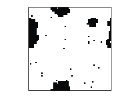
Figure 6: Non-equiprobable $64\times 64$ binary MRF, with $p_{0}=0.1$ and $\beta=-3.0$.

II-B2 Stochastic Relaxation

The stochastic relaxation algorithm of Geman and Geman (G&G) [1] is an iterative algorithm that proceeds at discrete time steps $t=0,1,2,\ldots,t_{\mathrm{max}}$; after each step, a new MRF estimate $\hat{F}(t)$ is obtained. For sufficiently large $t_{\mathrm{max}}$, the algorithm converges to a final estimate $\hat{F}$ that does not change appreciably for $t>t_{\mathrm{max}}$. The initial estimate $\hat{F}(0)$ is computed by thresholding the noisy image $G$ at $1/2$. Given estimate $\hat{F}(t)$ at time $t$, at time $t+1$ $M\times N$ randomly chosen pixels of $\hat{F}(t)$ are visited. The value of each pixel $(m,n)$ visited during the random scan is set to 0 or 1 with probability $1/2$. If the new value is different from its value $\hat{f}_{m,n}$ at time $t$, then the energy difference $\Delta\mathcal{E}_{P}(m,n)=\mathcal{E}_{P}(\mathrm{NOT}(\hat{f}_{m,n}))-\mathcal{E}_{P}(\hat{f}_{m,n})$ is computed. In computing $\Delta\mathcal{E}_{P}(m,n)$, only one pixel at a time (i.e., pixel $(m,n)$) is changed; all other pixels retain their values from time $t$. If $\Delta\mathcal{E}_{P}(m,n)<0$, then the change is accepted: $\hat{f}_{m,n}(t+1)=\mathrm{NOT}(\hat{f}_{m,n}(t))$. If $\Delta\mathcal{E}_{P}(m,n)\geq 0$, the change is accepted with probability $q=\exp\left[-\Delta\mathcal{E}_{P}(m,n)/T(t+1)\right]$. The temperature $T$ is gradually reduced according to a logarithmic annealing schedule: $T(t)=C/\log(1+t),1\leq t\leq t_{\mathrm{max}}$; in this paper the value $C=3.0$ is used for all simulations.

The modified (a posteriori) energy function $\mathcal{E}_{P}$ used by the MRF estimator at time $t+1$ includes the difference energy between the noisy input image $G$ and the current trial estimate:

$$\mathcal{E}_{P}(f_{m,n})=\mathcal{E}_{I}(f_{m,n})+\|G-\hat{F}(t,f_{m,n})\|^{2}/2\sigma_{G}^{2},$$ (9)

where $\hat{F}(t,f_{m,n})$ denotes the estimated MRF $\hat{F}(t)$ with pixel $(m,n)$ taking the value $f_{m,n}$, and $\sigma_{G}^{2}$ is estimated as in (5). The extrinsic information LLRs $L_{\mathrm{in}}^{\mathrm{MRF}}(m,n)=\log\left[\mathrm{Pr}_{\mathrm{ext}}(F_{m,n}=1)/\mathrm{Pr}_{\mathrm{ext}}(F_{m,n}=0)\right]$ represent independent a priori information about pixel $(m,n)$. Hence, in the $\mathcal{E}_{I}(f_{m,n})$ of (9), we replace $\alpha$ with

$$\alpha^{\prime}=\alpha-L_{\mathrm{in}}^{\mathrm{MRF}}(m,n).$$ (10)

After converting to probabilities using (6), this extra LLR term in $\alpha^{\prime}$ results in the corresponding extrinsic probabilities $\mathrm{Pr}_{\mathrm{ext}}(F_{m,n}=f_{m,n})$ appearing as independent weight factors in the renormalized expressions for the conditional probabilities of (6). Thus, as the LLRs $L_{\mathrm{in}}^{\mathrm{MRF}}(m,n)$ grow increasingly large with successive iterations of the concatenated detector, they increasingly influence the estimates $\hat{F}$ arrived at by the MRF detector.

The G&G algorithm provides only a binary estimate $\hat{F}$ of the MRF. To compute LLR estimates $L^{\mathrm{MRF}}(m,n)$ for each pixel, we use the following method, which is similar to that in [18, 19], where a soft-output G&G algorithm is used for recovery of noise-corrupted MRFs, and for iterative source-channel image decoding with MRF source models. After the stochastic relaxation algorithm convergences, we compute the conditional probabilities based on the MRF model:

$$\mathrm{Pr}(F_{m,n}=0|\mathcal{F}_{m,n})=\frac{1}{1+e^{-(\alpha^{\prime}+\beta v_{m,n})/T}}$$ (11)

$$\mathrm{Pr}(F_{m,n}=1|\mathcal{F}_{m,n})=\frac{e^{-(\alpha^{\prime}+\beta v_{m,n})/T}}{1+e^{-(\alpha^{\prime}+\beta v_{m,n})/T}}.$$ (12)

The LLRs $L^{\mathrm{MRF}}(m,n)$ are then computed as

$$L^{\mathrm{MRF}}(m,n) = -(\alpha^{\prime}+\beta v_{m,n})/T$$ (13)

$$= -\frac{(\alpha-L_{\mathrm{in}}^{\mathrm{MRF}}(m,n)+\beta v_{m,n})}{T}.$$

And since $L_{\mathrm{in}}^{\mathrm{MRF}}(m,n)$ is weighed by $1/T$,

$$L_{\mathrm{out}}^{\mathrm{MRF}}(m,n) = L^{\mathrm{MRF}}(m,n)-L_{\mathrm{in}}^{\mathrm{MRF}}(m,n)/T$$ (14)

$$= -(\alpha+\beta v_{m,n})/T.$$

III Simulation Results

In early iterations of the concatenated system of Fig. 2, the ISI detector cannot remove all the ISI from received image $r$. Due to its use of soft-decision feedback, the ISI detector is also subject to error propagation, especially at low SNRs. Thus, the “noisy image” $G$ supplied to the MRF detector by the ISI detector contains bit errors as well as Gaussian-like noise. To verify that the MRF detector can correct some of these bit errors (by exploiting the Markov structure of the image), we performed the simulation diagrammed in Fig. 7. The MRF passes through a binary-symmetric channel (BSC) with crossover probability $p$, followed by an AWGN channel, and is then detected with the MRF MAP estimator. Fig. 8 plots the BER of the hard decisions made at the MRF estimator’s output versus the SNR $10\log_{10}\left(\mbox{var}\left[F\right]/\sigma_{w}^{2}\right)$ of the AWGN channel, for several values of the BSC error probability $p$. In every case, the MRF detector’s output has an error floor lower than the value of $p$ used in the simulation. This result strongly suggests that the MRF detector can improve the reliability of the information passed to it by the ISI detector.

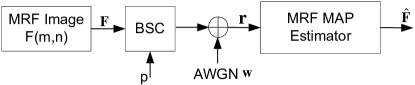
Figure 7: Experiment to test error correction capability of the MRF detector.

Figure 8: Simulation results for the experiment shown in Fig. 7.

All simulations of the concatenated system of Fig. 2 used the the $2\times 2$ averaging mask (with $h(k,l)=1/4$ for $0\leq(k,l)\leq 1$) in the 2D convolution of (1). All simulations used 5 outer iterations of the entire concatenated system, with one inner iteration of the ISI detector performed for each outer iteration. In the following subsections, we present simulation results for three cases: (1) the source image is a binary first order MRF, and the receiver knows the MRF parameters; (2) the source image is a binary first order MRF, and the receiver guesses the MRF parameters; and (3) the source image is a natural binary image, and the receiver guesses the most appropriate MRF parameters.

III-A MRF Source and Known Markov Parameters at the Receiver

Monte-Carlo simulation results for the concatenated system, when the source images were the two $64\times 64$ binary equiprobable MRFs shown in Fig. 5(c) and (d), are shown in Fig. 9. The SNR in Fig. 9 is defined as in [12]:

$$\mbox{SNR}=10\log_{10}\left(\mbox{var}\left[\tilde{F}\ast h\right]/\sigma_{w}^{2}\right),$$ (15)

where $\ast$ denotes 2D convolution, and $\sigma_{w}^{2}$ is the variance of the Gaussian r.v.s $w(m,n)$ in (1). The performance of the IRCSDF ISI detector alone on the received image $\mathbf{r}$ is also shown for comparison. When the BER is $2\times 10^{-5}$, the concatenated system gives SNR savings of $0.5$ and $1.5$ dB over the ISI detector alone, for images b and c respectively. As the input MRF becomes more correlated, the MRF detector makes increasingly reliable decisions, thereby improving the system’s SNR gain. At BER of $4\times 10^{-3}$, the concatenated system saves about $1.0$ and $2.7$ dB over the ISI detector alone, for images b and c respectively. The gains increase at lower SNR, where the additional input of the MRF detector helps the ISI detector resolve an increased number of ambiguous cases.

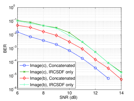
Figure 9: Simulation results for the concatenated system of Fig. 2 on the 2D ISI channel with $2\times 2$ averaging mask and AWGN, for MRFs b and c shown in Fig. 5. The performance of the ISI detector alone is also shown for comparison.

We also considered first order MRFs with non-equiprobable pixels. Fig. 10 shows simulation results on the $p_{0}=0.1$, $\beta=-3.0$ MRF of Fig. 6. The figure shows performance of the concatenated system, as well as the performances of the non-equiprobable and equiprobable ISI detectors alone. Non-equiprobable ISI detection offers little gain at high SNR, but saves between 0.5 and 1 dB at lower SNRs. The addition of the MRF detector (with modified $\alpha$ as in (8)) gives SNR savings of about 1 dB at BER $2\times 10^{-4}$, and about 3 dB at BER $10^{-2}$, over non-equiprobable ISI detection alone. A similar set of simulation results, but with $p_{0}=0.01$, is shown in Fig. 11. Now the gain of non-equiprobable ISI compared to equiprobable ISI detection is higher: about 0.5 dB at BER $10^{-4}$. But the gain of the concatenated system over non-equiprobable ISI is smaller: about 0.3 dB at BER $2\times 10^{-4}$. Clearly it is worth exploiting a non-uniform pixel distribution by using the non-equiprobable concatenated system in place of equiprobable ISI detection alone, although for extremely skewed distributions, non-equiprobable ISI detection alone achieves most of the available SNR gain.

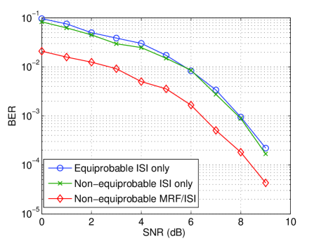
Figure 10: Simulation results for the concatenated system of Fig. 2 on the 2D ISI channel with $2\times 2$ averaging mask and AWGN, for the non-equiprobable MRF with $p_{0}=0.1$ and $\beta=-3.0$ shown in Fig. 6. The performances of the equiprobable and non-equiprobable ISI detectors alone are also shown for comparison.

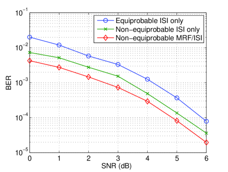
Figure 11: Simulation results for the concatenated system of Fig. 2 on the 2D ISI channel with $2\times 2$ averaging mask and AWGN, for a non-equiprobable MRF with $p_{0}=0.01$ and $\beta=-3.0$. The performances of the equiprobable and non-equiprobable ISI detectors alone are also shown for comparison.

It is also worth noting that the concatenated algorithm greatly outperforms the standard G&G algorithm applied to a non-interleaved MRF passed through the ISI channel. Simulation results for the G&G algorithm alone operating on a $\beta=-3.0$ MRF passed through the $2\times 2$ averaging-mask ISI channel are shown in Fig. 12. The SNR in this figure is defined by replacing $\tilde{F}$ by $F$ in (15). From the figure it is clear that the G&G algorithm alone has a BER floor of about $1.5\times 10^{-3}$, and thus is not suitable for 2D digital storage applications, where much lower BERs are required.

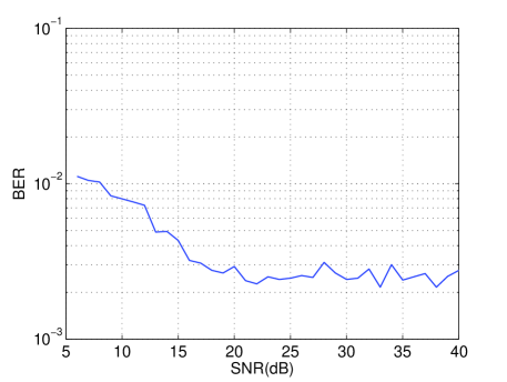
Figure 12: Simulation results for the standard Geman and Geman stochastic relaxation algorithm applied to a MRF with correlation parameter $\beta=-3.0$, that has passed through the 2D ISI channel with $2\times 2$ averaging mask and AWGN without being interleaved first.

III-B MRF Source and Unknown Markov Parameters at the Receiver

If the MRF detector must estimate the Markov model parameters, there will be some estimation error between the actual and estimated parameters. This leads to the question: how accurate must the model parameters be in order to achieve performance gains similar to those seen when the parameters are known exactly?

To answer this question, we did a number of simulations using the equiprobable MRFs of Fig. 5(b) and (c), in which the assumed MRF parameter $\beta$ did not match the actual parameter. These simulation results are shown in Figs. 13 and 14. In Fig. 13 the source image has $\beta=-1.5$. At high SNR, there is a mismatch penalty of about 0.2 or 0.3 dB when the receiver assumes that $\beta$ is one of the values $(-0.5,-0.75,-3.0)$, but this still leads to a gain of about 0.2 dB over the ISI-only case. Only when $\beta$ is assumed to be $-4.5$ does the concatenated system perform worse than the ISI detector alone. Interestingly, at low SNR, the assumed values of $-3.0$ and $-4.5$ give almost identical results to the correct value of $-1.5$. The concatenated system thus appears to be quite robust to receiver parameter mismatch, at both high and low SNRs.

The results shown in Fig. 14, where the source MRF has $\beta=-3.0$, suggest that robustness to parameter mismatch increases as the source MRF becomes more correlated. At high SNR, assumed values of $\beta$ in a range between $-1.5$ and $-10.0$ give gains of more than 1 dB compared to ISI-only detection; assumed values of $-4.5$ and $-6.0$ perform as well as the correct value of $\beta=-3.0$.

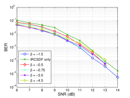
Figure 13: Simulation results for the concatenated system of Fig. 2 on the 2D ISI channel with $2\times 2$ averaging mask and AWGN, for the $\beta=-1.5$ binary MRF of Fig. 5(b) with receiver parameter mismatch.

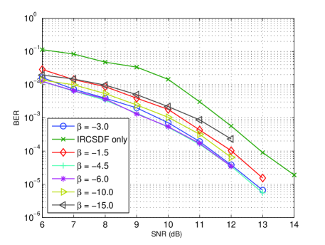
Figure 14: Simulation results for the concatenated system of Fig. 2 on the 2D ISI channel with $2\times 2$ averaging mask and AWGN, for the $\beta=-3.0$ binary MRF of Fig. 5(c) with receiver parameter mismatch.

III-C Natural Image Sources

We also tested the performance of our concatenated MRF-ISI detector on the two natural binary images “chair” and “man” shown in Fig. 15. In these images, the numbers of 0s and 1s are nearly equal, so we used the equiprobable version of the MRF-ISI system.

 

Figure 15: Two $64\times 64$ natural binary images: (a) chair, and (b) man.

Without doing any model estimation, we simply used our first order MRF model with several guessed values of $\beta$ (namely, $-1.5$, $-3.0$, $-4.5$, and $-6.0$) to model these two images. The simulation results for the chair and man images appear in Figs. 16 and 17. For these natural images at high SNR, the concatenated detector achieves SNR savings of between 1 and 2 dB compared to the ISI-only detector, for a wide choice of $\beta$ values at the receiver, thereby demonstrating that a simple first-order MRF model is very useful in reducing 2D ISI in natural binary images.

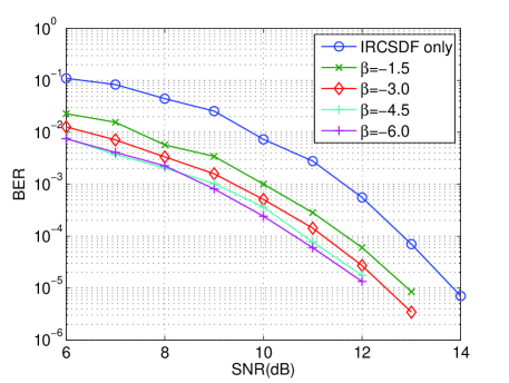
Figure 16: Simulation results for the concatenated system of Fig. 2 on the 2D ISI channel with $2\times 2$ averaging mask and AWGN, on the natural binary image “chair” of Fig. 15, for various values of MRF parameter $\beta$.

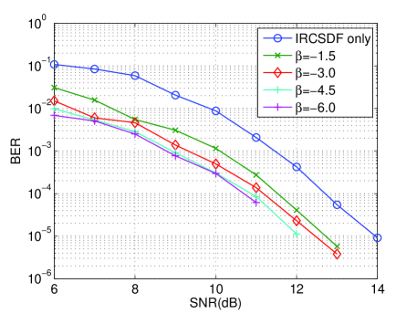
Figure 17: Simulation results for the concatenated system of Fig. 2 on the 2D ISI channel with $2\times 2$ averaging mask and AWGN, on the natural binary image “man” of Fig. 15, for various values of MRF parameter $\beta$.

IV Conclusion

This paper has demonstrated that, if the input image to a 2D ISI channel has 2D correlation that can be modeled by a MRF, then significant SNR savings over previously proposed 2D-ISI detectors can be realized by employing a concatenated iterative decoder consisting of SISO 2D-ISI and MRF detectors, and that the SNR savings increase with the degree of source-image correlation. The techniques described in this paper have potential application in future-generation optical recording systems, which will employ 2D read/write heads. In practice, many source images destined for storage on such media are correlated; for example, uncompressed natural images are usually highly correlated, and most practical image-compression schemes leave residual correlation. This paper has also demonstrated that the proposed algorithm is quite robust to MRF parameter mismatch between the source image and the receiver, and that the simple first-order MRF is a very useful model for 2D-ISI reduction in natural binary images. The basic ideas presented in this paper should extend to more realistic image models and more practical scenarios. Algorithms that learn an appropriately accurate MRF model from the source image would allow practical implementation of joint 2D-ISI and MRF estimators in optical storage systems; such algorithms are currently under investigation by the authors.

References

- [1] S. Geman and D. Geman, “Stochastic relaxation, Gibbs distributions, and the Bayesian restoration of images,” IEEE Trans. Pattern Analysis Mach. Intell., vol. PAMI-6, pp. 721–741, Nov. 1984.
- [2] G. T. Huang, “Holographic memory,” MIT Tech. Review, vol. 9, Sep. 2005. Available online at http://www.inphase-tech.com.
- [3] J. F. Heanue, K. Gürkan, and L. Hesselink, “Signal detection for page-access optical memories with intersymbol interference,” Applied Optics, vol. 35, pp. 2431–2438, May 1996.
- [4] R. Krishnamoorthi, “Two-dimensional Viterbi like algorithms,” Master’s thesis, Univ. Illinois at Urbana Champaign, 1998.
- [5] X. Chen and K. M. Chugg, “Near-optimal data detection for two-dimensional ISI/AWGN channels using concatenated modeling and iterative algorithms,” in Proc. IEEE International Conference on Communications, ICC’98, pp. 952–956, 1998.
- [6] C. L. Miller, B. R. Hunt, M. W. Marcellin, and M. A. Neifeld, “Image restoration using the Viterbi algorithm,” Journal of the Optical Society of America A, Vol. 16, No. 2, pp. 265-274, Feb. 2000.
- [7] M. Marrow and J. K. Wolf, “Iterative detection of 2-dimensional ISI channels,” in Proc. Info. Theory Workshop, (Paris, France), pp. 131–134, Mar./Apr. 2003.
-
[8]
M. Marrow, “Equalization and detection of 2-d ISI channels.” slide
presentation available at http://cmrr-wolf08.ucsd.edu/
~mmarrow/, May 2003. - [9] Y. Wu and J. A. O’Sullivan, “Iterative Detection and Decoding for Separable Two-Dimensional Intersymbol Interference,” IEEE Trans. Magnetics, Vol. 39, No.4, July 2003
- [10] O. Shental, A. J. Weiss, N. Shental, and Y. Weiss, “Generalized belief propagation receiver for near-optimum detection of two-dimensional channels with memory,” Proc. Info. Theory Workshop, (San Antonio, Texas), pp. 225–229, Oct. 2004.
- [11] Z. Zhao and R. E. Blahut, “The Richardson-Lucy algorithm based demodulation algorithms for the two-dimensional intersymbol interference channel,” in Proc. 39th Conf. on Info. Sci. and Systems (CISS’05), (CD-ROM), paper 83, Johns-Hopkins U., Mar. 2005.
- [12] T. Cheng, B. Belzer and K. Sivakumar, “Image deblurring with iterative row-column soft-decision feedback algorithm,” in Proc. 39th Conf. on Info. Sci. and Systems (CISS’05), (CD-ROM), paper 210, Johns-Hopkins U., Mar. 2005.
- [13] P. M. Njeim, T. Cheng, B. J. Belzer and K. Sivakumar, “Image detection in 2D intersymbol interference with iterative soft-decision feedback zig-zag algorithm,” in Proc. 43rd Allerton Conf. on Comm., Comp., and Control, (CD-ROM), U. of Illinois Urbana-Champaign, Sept. 2005.
- [14] T. Cheng, B. Belzer and K. Sivakumar, “An iterative row-column soft-decision feedback algorithm for two-dimensional intersymbol interference,” submitted to IEEE Sig. Proc. Letters, Nov. 2005.
- [15] C. Berrou and A. Glavieux, “Near optimum error correcting coding and decoding: turbo-codes,” IEEE Trans. Commun., vol. 44, pp. 1261 – 1271, Oct. 1996.
- [16] L. R. Bahl, J. Cocke, F. Jelinek, and J. Raviv, “Optimal decoding of linear codes for minimizing symbol error rate,” IEEE Trans. Info. Th., vol. 20, pp. 284–287, Mar. 1974.
- [17] G. R. Cross and A. K. Jain, “Markov Random Field Texture Models,” IEEE Trans. Pattern Analysis and Machine Intelligence, vol. PAMI-5, pp. 25–39, Jan. 1983.
- [18] A. Mertins, “Image recovery from noisy transmission using soft bits and Markov random field models,” Optical Engineering, vol. 42, pp. 2893-2899, Oct. 2003.
- [19] J. Kliewer, N. Gortz, and A. Mertins, “On iterative source-channel image decoding with Markov random field source models,” Proc. IEEE ICASSP 2004, vol. 4, pp. 661-664, May 2004.