Pseudo-Codeword Performance Analysis
for LDPC Convolutional Codes

Abstract

Message-passing iterative decoders for low-density parity-check (LDPC) block codes are known to be subject to decoding failures due to so-called pseudo-codewords. These failures can cause the large signal-to-noise ratio performance of message-passing iterative decoding to be worse than that predicted by the maximum-likelihood decoding union bound.

In this paper we address the pseudo-codeword problem from the convolutional-code perspective. In particular, we compare the performance of LDPC convolutional codes with that of their “wrapped” quasi-cyclic block versions and we show that the minimum pseudo-weight of an LDPC convolutional code is at least as large as the minimum pseudo-weight of an underlying quasi-cyclic code. This result, which parallels a well-known relationship between the minimum Hamming weight of convolutional codes and the minimum Hamming weight of their quasi-cyclic counterparts, is due to the fact that every pseudo-codeword in the convolutional code induces a pseudo-codeword in the block code with pseudo-weight no larger than that of the convolutional code’s pseudo-codeword. This difference in the weight spectra leads to improved performance at low-to-moderate signal-to-noise ratios for the convolutional code, a conclusion supported by simulation results.

Submitted to IEEE Transactions on Information Theory, September 2006

Index terms — Convolutional codes, quasi-cyclic codes, low-density parity-check (LDPC) codes, linear programming decoding, message-passing iterative decoding, pseudo-codewords, pseudo-weights.

1 Introduction

Although low-density parity-check block codes (LDPC-BCs) have very good performance under message-passing iterative (MPI) decoding, they are known to be subject to decoding failures due to so-called pseudo-codewords. These are real-valued vectors that can be loosely described as error patterns that cause non-convergence in iterative decoding due to the fact that the algorithm works locally and can give priority to a vector that fulfills the equations of a graph cover rather than the graph itself.

Example 1.1.

Consider the trivial length-$3$ and dimension-$0$ code $\mathsf{C}=\{(0,0,0)\}$ defined by the $3\times 3$ parity-check matrix

$$\mathbf{H} \triangleq\begin{bmatrix}1&1&0\\ 1&1&1\\ 0&1&1\end{bmatrix}$$ (1.1)

and whose Tanner graph is shown in Fig. 1 (left). A possible cubic cover of this Tanner graph is also depicted in Fig. 1 (right). Because $(1{:}1{:}0,\ 1{:}1{:}0,\ 1{:}1{:}0)$ is a valid configuration in this cubic cover, the vector $\boldsymbol{\omega}=\bigl{(}\frac{2}{3},\frac{2}{3},\frac{2}{3}\bigr{)}$ is a pseudo-codeword of the code $\mathsf{C}$ defined by $\mathbf{H}$ (see [2, 3]). $\square$

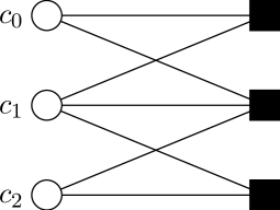
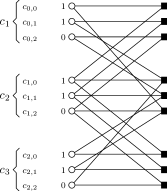
Figure 1: Left: the Tanner graph associated with the parity-check matrix $\mathbf{H}$ that was defined in (1.1). Right: $(1{:}1{:}0,\ 1{:}1{:}0,\ 1{:}1{:}0)$ is a valid codeword in a cubic cover.

It has been shown [2, 4, 5] that the performance of MPI decoding schemes for LDPC-BCs is largely dominated not by minimum Hamming weight considerations but by minimum pseudo-weight considerations, where the minimum pseudo-weight in the case of an additive white Gaussian noise channel (AWGNC) is defined as $w_{\mathrm{p}}^{\mathrm{min}}(\mathbf{H})\triangleq\min_{\boldsymbol{\omega}\in\mathcal{P}\atop\boldsymbol{\omega}\neq\mathbf{0}}\frac{\lVert\boldsymbol{\omega}\rVert_{1}^{2}}{\lVert\boldsymbol{\omega}\rVert_{2}^{2}},$ where $\lVert\,\cdot\,\rVert_{1}$ and $\lVert\,\cdot\,\rVert_{2}$ are, respectively, the $1$-norm and $2$-norm, and $\mathcal{P}$ is the set of all pseudo-codewords for the code $\mathsf{C}$ defined by $\mathbf{H}$. The minimum pseudo-weight is a measure of the effect that decoding failures have on the performance of the code. As a consequence, the large signal-to-noise ratio (SNR) performance of MPI decoding can be worse than that predicted by the maximum-likelihood decoding union bound, which constitutes a major problem when trying to determine performance guarantees. Addressing this problem from the convolutional-code perspective, i.e., studying the pseudo-codeword problem described above for LDPC convolutional codes (LDPC-CCs), constitutes the major topic of this paper.

Figure 2: The MPI decoding performance of a rate $R=2/5$ $(3,5)$-regular LDPC convolutional code and three associated $(3,5)$-regular QC-LDPC block codes. (Maximum of $50$ iterations.)

We investigate a class of time-invariant LDPC convolutional codes derived by “unwrapping” certain classes of quasi-cyclic (QC) LDPC block codes that are known to have good performance [6, 7, 8]. Unwrapping a QC block code to obtain a time-invariant convolutional code represents a major link between QC block codes and convolutional codes. This link was first introduced in a paper by Tanner [9], where it was shown that the free distance of the unwrapped convolutional code, if non-trivial, cannot be smaller than the minimum distance of the underlying QC code. This idea was later extended in [10, 11]. More recently, a construction for LDPC convolutional codes based on QC-LDPC block codes was introduced by Tanner et al. [7, 6], and a sliding-window MPI decoder was described. In that paper it was noted that the (non-trivial) convolutional versions of these codes significantly outperformed their block code counterparts in the waterfall region of the bit error rate (BER) curve, even though the graphical representations of MPI decoders were essentially equivalent.

Throughout this paper we mainly take the approach of [2, 3, 14], which connects the presence of pseudo-codewords in MPI decoding and linear programming (LP) decoding. LP decoding was introduced by Feldman, Wainwright, and Karger [15, 16] and can be seen as a relaxation of the maximum-likelihood decoding problem. More precisely, maximum-likelihood decoding can be formulated as the solution to an optimization problem, where a linear cost function is minimized over a certain polytope, namely the polytope that is spanned by the set of all codewords. For general codes, there is no efficient description of this polytope and so Feldman et al. suggested replacing it with an (efficiently describable) relaxed polytope, which in the following will be called the “fundamental polytope”. In other words, the decoding result of the LP decoder is the point in the fundamental polytope that minimizes the above-mentioned linear cost function.

In order to analyze the behavior of unwrapped LDPC convolutional codes under LP decoding, we need to examine the fundamental polytope [2, 3] of the underlying QC-LDPC block codes. (Because of symmetries, it is actually sufficient to study the structure of the fundamental polytope around the zero codeword, i.e., it is sufficient to study the so-called fundamental cone.) Our goal is to formulate analytical results (or at least efficient procedures) that will allow us to bound the minimum pseudo-weight of the pseudo-codewords of the block and convolutional codes.

The paper aims at addressing this question and related issues. In the following sections, we will study the connections that exist between pseudo-codewords in QC codes and pseudo-codewords in the associated convolutional codes and show that this connection mimics the connection between the codewords in QC codes and the associated convolutional codes.

1.1 Motivational Example

As a motivational example we simulated a rate $R=2/5$ $(3,5)$-regular LDPC-CC with syndrome former memory $m_{\text{s}}=21$, together with three wrapped block code versions: a $[155,64]$ $(3,5)$-regular QC-LDPC block code, a $[200,82]$ code, and a $[240,98]$ code, with parity-check matrices of increasing circulant sizes $r=31$, $r=40$, and $r=48$, respectively, while keeping the same structure within each $r\times r$ circulant [1] (see Section 2.1). (Note that increasing the circulant size of the QC code increases its complexity, i.e., its block length. Also note that each of the three block codes has rate slightly greater than $2/5$.) A sliding-window MPI decoder as in [6] was used to decode the convolutional code. Conventional LDPC-BC MPI decoders were employed to decode the QC-LDPC block codes. All decoders were allowed a maximum of $50$ iterations. The resulting BER performance of these codes on a binary-input AWGN channel is shown in Fig. 2.

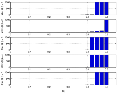
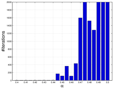
Figure 3: Left: Number of iterations needed for a sum-product-algorithm-type MPI decoder to decide for the all-zero codeword. ($1000$ corresponds to no convergence.) Here the $\beta$ values $1.00$, $2.00$, $3.00$, $4.00$, $5.00$ correspond to signal-to-noise ratios $E_{\mathrm{b}}/N_{0}$ of, respectively, $-2.04\ \mathrm{dB}$, $0.96\ \mathrm{dB}$, $2.73\ \mathrm{dB}$, $3.97\ \mathrm{dB}$, $4.94\ \mathrm{dB}$. Right: Number of iterations needed for a min-sum-algorithm-type MPI decoder to decide for the all-zero codeword. ($2000$ corresponds to no convergence.) We did not observe convergence to the all-zero codeword for $\alpha>0.50$ either for the sum-product-algorithm-type MPI decoder or for the min-sum-algorithm-type MPI decoder.

We note that, particularly in the low-to-moderate SNR region, where the complete pseudo-weight spectrum plays an important role, the unwrapped LDPC-CC performs between $0.5\ \mathrm{dB}$ and $1.0\ \mathrm{dB}$ better than the associated QC-LDPC block codes. Also, as the circulant size increases, the performance of the block codes approaches that of the convolutional code. These performance curves suggest that the pseudo-codewords in the block code that result in decoding failures may not cause such failures in the convolutional code, which suggests that LDPC-CCs may have better iterative decoding thresholds than comparable LDPC-BCs (see also [12] and [13]).

In order to underline the influence of pseudo-codewords under MPI decoding, we consider the following experiment. Let $\boldsymbol{\omega}$ be a minimal pseudo-codeword [3] for the above-mentioned $R=2/5$ $(3,5)$-regular LDPC-CC, i.e., a pseudo-codeword that corresponds to an edge of the fundamental cone of that LDPC-CC. Moreover, we define the log-likelihood ratio vector $\boldsymbol{\lambda}(\alpha,\beta)$ to be

$$\boldsymbol{\lambda}(\alpha,\beta) \triangleq\beta\cdot\left(\mathbf{1}-2\alpha\frac{\lVert\boldsymbol{\omega}\rVert_{1}}{\lVert\boldsymbol{\omega}\rVert_{2}^{2}}\boldsymbol{\omega}\right).$$

We then run the MPI decoder that is initialized with $\boldsymbol{\lambda}=\boldsymbol{\lambda}(\alpha,\beta)$ and count how many iterations it takes until the decoder decides for the all-zero codeword as a function of $\alpha$ and $\beta$. The results are shown in Fig. 3.

The meaning of $\boldsymbol{\lambda}(\alpha,\beta)$ is the following. If $\alpha=0$, then $\boldsymbol{\lambda}$ corresponds to the log-likelihood ratio vector that the receiver sees when the communication system operates at a signal-to-noise ratio $E_{\mathrm{b}}/N_{0}=\beta/(4R)$ and when the noise vector that is added by the binary-input AWGN channel happens to be the all-zero vector (see, e.g., the discussion in [3, Sec. 3]). For non-zero $\alpha$ the expression for $\boldsymbol{\lambda}(\alpha,\beta)$ has been set up such that the LP decoder has a decision boundary at $\alpha=0.5$: for $\alpha<0.5$ the all-zero codeword wins against the pseudo-codeword $\boldsymbol{\omega}$ whereas for $\alpha>0.5$ the all-zero codeword loses against the pseudo-codeword $\boldsymbol{\omega}$ under LP decoding.

The simulations in Fig. 3 were obtained using a search algorithm that looked for a low-pseudo-weight minimal pseudo-codeword $\boldsymbol{\omega}$ in the fundamental cone of the above-mentioned LDPC-CC. The $\boldsymbol{\omega}$ that we found has AWGNC pseudo-weight $18.1297$, which happens to be smaller than the free distance. Secondly, we ran the MPI decoder for various choices of $\alpha$ and $\beta$: Fig. 3 Left shows the number of iterations needed using a sum-product-algorithm-type MPI decoder whereas Fig. 3 Right shows the number of iterations needed using a min-sum-algorithm-type MPI decoder. (Note that the decisions reached by the latter are independent of the choice of $\beta$, $\beta>0$.) Because of the more oscillatory behavior of the min-sum-algorithm-type MPI decoder close to decision boundaries of the LP decoder, observed empirically, it is advantageous to run that decoder for many iterations in our scenario, whereas in the case of the sum-product-algorithm-type MPI decoder it hardly pays to go beyond $150$ iterations.

1.2 Paper Goals and Structure

In this paper, we provide a possible explanation for the performance difference observed in the motivational example above. Based on the results of [2, 3] that relate code performance to the existence of pseudo-codewords, we examine the pseudo-codeword weight spectra of QC-LDPC block codes and their associated convolutional codes. We will show that for a non-trivial LDPC-CC derived by unwrapping a non-trivial QC-LDPC block code, the minimum pseudo-weight of the convolutional code is at least as large as the minimum pseudo-weight of the underlying QC code[1], i.e.,

$$w_{\mathrm{p}}^{\mathrm{min}}\left(\mathbf{H}_{\mathrm{QC}}^{(r)}\right) \leq w_{\mathrm{p}}^{\mathrm{min}}\left(\mathbf{H}_{\mathrm{conv}}\right).$$

This result, which parallels the well-known relationship between the free Hamming distance of non-trivial convolutional codes and the minimum Hamming distance of their non-trivial quasi-cyclic counterparts [9], is based on the fact that every pseudo-codeword in the convolutional code induces a pseudo-codeword in the block code with pseudo-weight no larger than that of the convolutional code’s pseudo-codeword. This difference in the weight spectra leads to improved BER performance at low-to-moderate SNRs for the convolutional code, a conclusion supported by the simulation results presented in Fig. 2.

The paper is structured as follows. In Sec. 2 we develop the background necessary to describe the connection between pseudo-codewords in unwrapped LDPC convolutional codes and those in the associated QC-LDPC codes. Thus, in Sec. 2.1 we briefly discuss the connection between convolutional codes and their associated QC codes, especially how codewords in the former can be used to construct codewords in the latter, and in Sec. 2.2 we define the fundamental polytope/cone of a matrix and show how we can describe the fundamental cone of a polynomial parity-check matrix through polynomial inequalities. We end the section by showing how pseudo-codewords in unwrapped LDPC convolutional codes yield pseudo-codewords in the associated QC-LDPC codes. In Sec. 3, we compare the pseudo-weights of unwrapped convolutional and their associated QC block codes. Sec. 3.1 introduces various channel pseudo-weights and Sec. 3.2 presents the main result, namely that the minimum AWGN pseudo-weight, the minimum binary erasure channel (BEC) pseudo-weight, the minimum binary symmetric channel (BSC) pseudo-weight, and the minimum max-fractional weight of a convolutional code are at least as large as the corresponding minimum pseudo-weights of a wrapped QC block code. Sec. 4 discusses a method to analyze problematic pseudo-codewords, i.e., pseudo-codewords with small pseudo-weight. The method addresses the convolutional code case. It introduces two sequences of “truncated” pseudo-weights and, respectively, “bounded pseudo-codeword” pseudo-weights, that play an important role in identifying the minimum pseudo-weight of the convolutional code, similar to the role that column distances and row distances play in identifying the free distance. We end with some conclusions in Sec. 5.

1.3 Notation

Throughout the paper we will use the standard way of associating a Tanner graph with a parity-check matrix and vice-versa. We will use the following notation. We let $\mathbb{F}_{2}$, $\mathbb{R}$, $\mathbb{R}_{+}$, and $\mathbb{R}_{++}$ be the Galois field of size $2$, the field of real numbers, the set of non-negative real numbers, and the set of positive real numbers, respectively. If $a(X)$ is a polynomial over some field and $r$ is some positive integer then $\big{(}a(X)\operatorname{mod}\,(X^{r}-1)\big{)}$ denotes the polynomial $b(X)$ of degree smaller than $r$ such that $b(X)=a(X)\ (\mathrm{mod}\ (X^{r}-1))$. We say that a polynomial $\omega_{\ell}(D)=\sum_{i}\omega_{\ell,i}D^{i}$ with real coefficients is non-negative, and we write $\omega_{\ell}(D)\geq 0$, if all its coefficients $\omega_{\ell,i}$ satisfy $\omega_{\ell,i}\geq 0$. Similarly, a polynomial vector $\boldsymbol{\omega}(D)=\bigl{(}\omega_{1}(D),\omega_{2}(D),\ldots,\omega_{L}(D)\bigr{)}$ is non-negative, and we write $\boldsymbol{\omega}(D)\geq\mathbf{0}$, if all its polynomial components $\omega_{\ell}(D)$ satisfy $\omega_{\ell}(D)\geq 0$ for all $\ell\in\{1,\ldots,L\}$. Moreover, a polynomial matrix $\mathbf{A}(D)$ is non-negative, and we write $\mathbf{A}(D)\geq\mathbf{0}$, if all its entries are non-negative polynomials. Finally, for any positive integer $r$ and for any $r^{\prime}\in\{0,1,\ldots,r-1\}$, $\mathbf{I}_{r^{\prime}}$ will represent the $r^{\prime}$-times cyclically left-shifted identity matrix of size $r\times r$.

2 Pseudo-Codewords for QC and Convolutional Codes

We begin this section by presenting an important link between QC block codes and convolutional codes that was first introduced in a paper by Tanner [9] and later extended in [10, 11]. Similar to the connection between codewords in an unwrapped convolutional code and codewords in the underlying QC code, we will show that pseudo-codewords in the convolutional code give pseudo-codewords when projected onto an underlying QC code.

2.1 A Link Between QC Block Codes and Convolutional Codes

In this section we introduce the background needed for the later development of the paper. Note that all codes will be binary linear codes.

Any length $n\triangleq r\cdot L$ quasi-cyclic (QC) code $\mathsf{C}_{\rm QC}\triangleq\mathsf{C}_{\mathrm{QC}}^{(r)}$ with period $L$ can be represented by an $rJ\times rL$ scalar block parity-check matrix $\mathbf{H}_{\mathrm{QC}}^{(r)}$ that consists of $J\times L$ circulant matrices of size $r\times r$. Using the isomorphism between the ring of binary circulant matrices of size $r\times r$ and the ring of polynomials $\mathbb{F}_{2}[X]/\langle X^{r}-1\rangle$ of degree less than $r$, we can associate with the scalar parity-check matrix $\mathbf{H}_{\mathrm{QC}}^{(r)}$ the polynomial parity-check matrix $\mathbf{H}_{\mathrm{QC}}^{(r)}(X)\in\big{(}\mathbb{F}_{2}[X]/\langle X^{r}-1\rangle\big{)}^{J\times L}$, with polynomial operations performed modulo $X^{r}-1$. Due to the existence of this isomorphism, we can identify two descriptions, scalar and polynomial, and use either of the two depending on their usefulness.

Example 2.1.

The cubic cover $\mathsf{C^{(3)}}$ of the trivial code in depicted in Fig. 1 is a quasi-cyclic code with scalar parity-check matrix $\mathbf{H}_{\mathrm{QC}}^{(3)}$ and corresponding polynomial parity-check matrix $\mathbf{H}_{\mathrm{QC}}^{(3)}(X)\in\big{(}\mathbb{F}_{2}[X]/\langle X^{r}-1\rangle\big{)}^{3\times 3}$ ($r=3$) given by

$$\mathbf{H}_{\mathrm{QC}}^{(3)}= \begin{bmatrix}1&0&0&1&0&0&0&0&0\\ 0&1&0&0&1&0&0&0&0\\ 0&0&1&0&0&1&0&0&0\\ 0&1&0&1&0&0&0&0&1\\ 0&0&1&0&1&0&1&0&0\\ 1&0&0&0&0&1&0&1&0\\ 0&0&0&1&0&0&1&0&0\\ 0&0&0&0&1&0&0&1&0\\ 0&0&0&0&0&1&0&0&1\end{bmatrix}=\begin{bmatrix}\mathbf{I}_{0}&\mathbf{I}_{0}&\mathbf{0}\\ \mathbf{I}_{2}&\mathbf{I}_{0}&\mathbf{I}_{1}\\ \mathbf{0}&\mathbf{I}_{0}&\mathbf{I}_{0}\end{bmatrix},\mathbf{H}_{\mathrm{QC}}^{(3)}(X)=\begin{bmatrix}1&1&0\\ X^{2}&1&X\\ 0&1&1\end{bmatrix}.$$ (2.1)

$\square$

By permuting the rows and columns of the scalar parity-check matrix $\mathbf{H}_{\mathrm{QC}}^{(r)}$ (i.e., by taking the first row in the first block of $r$ rows, the first row of the second block of $r$ rows, etc., then the second row in the first block, the second row in the second block, etc., and similarly for the columns), we obtain the parity-check matrix $\overline{\mathbf{H}}_{\mathrm{QC}}^{(r)}$ of a code that is equivalent to $\mathsf{C}_{\mathrm{QC}}^{(r)}$. The scalar parity-check matrix $\overline{\mathbf{H}}_{\mathrm{QC}}^{(r)}$ has the form

$$\overline{\mathbf{H}}_{\mathrm{QC}}^{(r)} \triangleq\begin{bmatrix}\mathbf{H}_{0}&\mathbf{H}_{r-1}&\cdots&\cdots&\mathbf{H}_{2}&\mathbf{H}_{1}\\ \mathbf{H}_{1}&\mathbf{H}_{0}&\cdots&\cdots&\mathbf{H}_{3}&\mathbf{H}_{2}\\ \vdots&\vdots&\ddots&&\vdots&\vdots\\ \vdots&\vdots&&\ddots&\vdots&\vdots\\ \mathbf{H}_{r-2}&\mathbf{H}_{r-3}&\cdots&\cdots&\mathbf{H}_{0}&\mathbf{H}_{r-1}\\ \mathbf{H}_{r-1}&\mathbf{H}_{r-2}&\cdots&\cdots&\mathbf{H}_{1}&\mathbf{H}_{0}\end{bmatrix},$$

where the scalar $J\times L$-matrices $\mathbf{H}_{0},\mathbf{H}_{1},\ldots,\mathbf{H}_{r-1}$ satisfy $\mathbf{H}_{\mathrm{QC}}^{(r)}(X)=\mathbf{H}_{0}+\mathbf{H}_{1}X+\cdots+\mathbf{H}_{r-1}X^{r-1}$.

Example 2.2.

The code in Example 2.1 has $\mathbf{H}_{\mathrm{QC}}^{(3)}(X)=\mathbf{H}_{0}+\mathbf{H}_{1}X+\mathbf{H}_{2}X^{2}$, where

$$\mathbf{H}_{0} \triangleq\begin{bmatrix}1&1&0\\ 0&1&0\\ 0&1&1\end{bmatrix},\mathbf{H}_{1}\triangleq\begin{bmatrix}0&0&0\\ 0&0&1\\ 0&0&0\end{bmatrix},\mathbf{H}_{2}\triangleq\begin{bmatrix}0&0&0\\ 1&0&0\\ 0&0&0\end{bmatrix}.$$ (2.2)

$\square$

Given the polynomial parity-check matrix of a QC-code, it is easy to see the natural connection that exists between quasi-cyclic codes and convolutional codes (see, e.g., [9, 10, 11, 7, 17]). Briefly, with any QC block code $\mathsf{C}_{\mathrm{QC}}^{(r)}$ of length $r\cdot L$, given by a $J\times L$ polynomial matrix parity-check matrix $\mathbf{H}_{\rm QC}^{(r)}(X)=\mathbf{H}_{0}+\mathbf{H}_{1}X+\cdots+\mathbf{H}_{r-1}X^{r-1}$, with polynomial operations performed modulo $X^{r}-1$, we can associate a rate $(L-J)/L$ convolutional code $\mathsf{C}_{\mathrm{conv}}$ given by the same $J\times L$ polynomial parity-check matrix $\mathbf{H}_{\mathrm{conv}}(D)=(h_{jl}(D))_{J\times L}=\mathbf{H}_{\mathrm{QC}}^{(r)}(D)=\mathbf{H}_{0}+\mathbf{H}_{1}D+\cdots+\mathbf{H}_{r-1}D^{r-1}$, where the change of variables indicates the lack of modulo $D^{r}-1$ operations [6]. Let the syndrome former memory $m_{\mathrm{s}}\leq r-1$ of $\mathsf{C}_{\mathrm{conv}}$ be the largest integer in $\{0,1,\ldots,r-1\}$ such that $\mathbf{H}_{m_{\mathrm{s}}}\neq 0$. Then the polynomial parity-check matrix $\mathbf{H}_{\mathrm{conv}}(D)$ has the following scalar description (see, e.g., [18])

$$\overline{\mathbf{H}}_{\mathrm{conv}} \triangleq\begin{bmatrix}\mathbf{H}_{0}&&&\\ \mathbf{H}_{1}&\mathbf{H}_{0}&&\\ \mathbf{H}_{2}&\mathbf{H}_{1}&\mathbf{H}_{0}&\\ \vdots&\vdots&\vdots&\ddots\\ \vdots&\vdots&\vdots&\ddots\\ \mathbf{H}_{r-1}&\mathbf{H}_{r-2}&\mathbf{H}_{r-3}&\ddots\\ &\mathbf{H}_{r-1}&\mathbf{H}_{r-2}&\ddots\\ &&\mathbf{H}_{r-1}&\ddots\\ &&&\ddots\end{bmatrix}=\begin{bmatrix}\mathbf{H}_{0}&&&\\ \mathbf{H}_{1}&\mathbf{H}_{0}&&\\ \mathbf{H}_{2}&\mathbf{H}_{1}&\mathbf{H}_{0}&\\ \vdots&\vdots&\vdots&\ddots\\ \mathbf{H}_{m_{\mathrm{s}}}&\mathbf{H}_{m_{\mathrm{s}}-1}&\mathbf{H}_{m_{\mathrm{s}}-2}&\ddots\\ &\mathbf{H}_{m_{\mathrm{s}}}&\mathbf{H}_{m_{\mathrm{s}}-1}&\ddots\\ &&\mathbf{H}_{m_{\mathrm{s}}}&\ddots\\ &&&\ddots\end{bmatrix}.$$

(Note that $\overline{\mathbf{H}}_{\mathrm{conv}}$ is a semi-infinite parity-check matrix.)

Example 2.3.

Unwrapping the code in Example 2.1, we obtain a convolutional code with polynomial parity-check matrix $\mathbf{H}_{\mathrm{conv}}$ given by

$$\mathbf{H}_{\mathrm{conv}}(D)= \begin{bmatrix}1&1&0\\ D^{2}&1&D\\ 0&1&1\end{bmatrix}.$$ (2.3)

The syndrome former memory is equal to 2 and the decomposition leading to the scalar matrix $\overline{\mathbf{H}}_{\mathrm{conv}}$ is $\mathbf{H}_{\mathrm{conv}}=\mathbf{H}_{0}+\mathbf{H}_{1}D+\mathbf{H}_{2}D^{2},$ where $\mathbf{H}_{0},\mathbf{H}_{1},\mathbf{H}_{2}$ are the same matrices as in (2.2). $\square$

In the same way as we obtained $\mathsf{C}_{\mathrm{conv}}$ from $\mathsf{C}_{\mathrm{QC}}^{(r)}$, we can, upon choosing a positive integer $r$, obtain a code $\mathsf{C}_{\mathrm{QC}}^{(r)}(X)$ from a given code $\mathsf{C}_{\mathrm{conv}}(D)$. It easily follows that, similar to obtaining $\overline{\mathbf{H}}_{\mathrm{conv}}$ by unwrapping $\overline{\mathbf{H}}_{\mathrm{QC}}^{(r)}$, $\overline{\mathbf{H}}_{\mathrm{QC}}^{(r)}$ is obtained from $\overline{\mathbf{H}}_{\mathrm{conv}}$ by suitably wrapping $\overline{\mathbf{H}}_{\mathrm{conv}}$. This unwrapping/wrapping can also be observed in the Tanner graph representations of $\mathbf{H}_{\mathrm{QC}}^{(r)}(X)$ and $\mathbf{H}_{\mathrm{conv}}(D)$, as illustrated in Fig. 4.

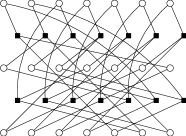
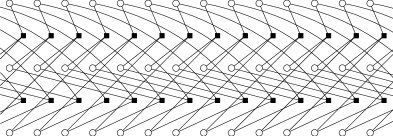
Figure 4: Left: The finite Tanner graph of a QC code. Right: The infinite Tanner graph of an unwrapped convolutional code.

We turn now our attention to codewords in these codes. Codewords in $\mathsf{C}_{\mathrm{QC}}^{(r)}$ will be denoted by a polynomial vector like $\mathbf{c}(X)$ and codewords in $\mathsf{C}_{\mathrm{conv}}$ will be denoted by a polynomial vector like $\mathbf{c}(D)$ (when the code is represented by a scalar parity-check matrix $\overline{\mathbf{H}}_{\mathrm{conv}}$, then it will be denoted by a vector like $\overline{\mathbf{c}}$). (We will later use a similar notation for pseudo-codewords.)

For any non-zero codeword $\mathbf{c}(D)$ with finite support in the convolutional code, its $r$ wrap-around, defined by the vector $\mathbf{c}(X)\operatorname{mod}\,(X^{r}-1)\in\big{(}\mathbb{F}_{2}[X]/\langle X^{r}-1\rangle\big{)}^{L}$, is a codeword in the associated QC-code, since $\mathbf{H}_{\mathrm{QC}}^{(r)}(X)\cdot\mathbf{c}(X)=\mathbf{0}$ in $\big{(}\mathbb{F}_{2}[X]/\langle X^{r}-1\rangle\big{)}^{L}$.

In addition, the Hamming weight of the two codewords is linked by the following inequality $w_{\mathrm{H}}\big{(}\mathbf{c}(X)\operatorname{mod}\,(X^{r}-1)\big{)}\leq w_{\mathrm{H}}(\mathbf{c}(D))$, which gives the inequality [9, 10] (we assume all codes are non-trivial)

$$d_{\mathrm{min}}\left(\mathsf{C}_{\mathrm{QC}}^{(r)}\right) \leq d_{\mathrm{free}}\left(\mathsf{C}_{\mathrm{conv}}\right)\quad\quad\text{ for all $r\geq m_{\mathrm{s}}+1$}.$$

Moreover, we have the following inequalities.

Lemma 2.4.

$$d_{\mathrm{min}}\left(\mathsf{C}_{\mathrm{QC}}^{(r)}\right) \leq d_{\mathrm{min}}\left(\mathsf{C}_{\mathrm{QC}}^{(2r)}\right)\leq d_{\mathrm{min}}\left(\mathsf{C}_{\mathrm{QC}}^{(4r)}\right)\leq\ \cdots\quad\quad\text{for all $r\geq m_{\mathrm{s}}+1$},$$

and

$$\lim_{r\rightarrow\infty}d_{\mathrm{min}}\left(\mathsf{C}_{\mathrm{QC}}^{(r)}\right) =d_{\mathrm{free}}\left(\mathsf{C}_{\mathrm{conv}}\right).$$

Proof: Let $\mathbf{H}_{\mathrm{QC}}^{(2r)}(X)$ be a parity-check matrix of $\mathsf{C}_{\mathrm{QC}}^{(2r)}$ and $\mathbf{H}_{\mathrm{QC}}^{(r)}(X)\triangleq\mathbf{H}_{\mathrm{QC}}^{(2r)}(X)\operatorname{mod}\,(X^{r}-1)$ be the corresponding parity-check matrix of $\mathsf{C}_{\mathrm{QC}}^{(r)}$. Let $\mathbf{c}(X)$ be a nonzero codeword in $\mathsf{C}_{\mathrm{QC}}^{(2r)}$ of weight equal to the minimum distance $d_{\mathrm{min}}\left(\mathsf{C}_{\mathrm{QC}}^{(2r)}\right)$. We have $\mathbf{H}_{\mathrm{QC}}^{(2r)}(X)\cdot\mathbf{c}(X)=\mathbf{0}$ in $\big{(}\mathbb{F}_{2}[X]/\langle X^{2r}-1\rangle\big{)}^{L}$ and since $X^{r}-1|X^{2r}-1$, it follows that $\mathbf{H}_{\mathrm{QC}}^{(r)}(X)\cdot\mathbf{c}(X)=\mathbf{0}$ in $\big{(}\mathbb{F}_{2}[X]/\langle X^{r}-1\rangle\big{)}^{L}$.

If $\mathbf{c}(X)\operatorname{mod}\,(X^{r}-1)\neq\mathbf{0}$ then we obtain the inequality $d_{\mathrm{min}}\left(\mathsf{C}_{\mathrm{QC}}^{(r)}\right)\leq d_{\mathrm{min}}\left(\mathsf{C}_{\mathrm{QC}}^{(2r)}\right).$ If $\mathbf{c}(X)=\mathbf{0}\operatorname{mod}\,(X^{r}-1)$ we can write $\mathbf{c}(X)=(X^{r}-1)\mathbf{c}_{1}(X)$ with $\mathbf{c}_{1}(X)\neq\mathbf{0}\operatorname{mod}\,(X^{r}-1)$ (otherwise $\mathbf{c}(X)=\mathbf{0}\operatorname{mod}\,(X^{2r}-1)$.) Hence $\mathbf{H}_{\mathrm{QC}}^{(r)}(X)\cdot(X^{r}-1)\cdot\mathbf{c}_{1}(X)=\mathbf{0}\operatorname{mod}\,(X^{2r}-1)$ or equivalently, $\mathbf{H}_{\mathrm{QC}}^{(r)}(X)\cdot\mathbf{c}_{1}(X)=\mathbf{0}\operatorname{mod}\,(X^{r}-1)$, which implies that $\mathbf{c}_{1}(X)$ is a nonzero codeword in $\mathsf{C}_{\mathrm{QC}}^{(r)}$. The Hamming weight $d_{\mathrm{min}}\left(\mathsf{C}_{\mathrm{QC}}^{(2r)}\right)=w_{\mathrm{H}}\big{(}\mathbf{c}(X)\big{)}=w_{\mathrm{H}}\big{(}(X^{r}-1)\mathbf{c}_{1}(X)\big{)}\geq 2\cdot w_{\mathrm{H}}(\mathbf{c}_{1}(X)\operatorname{mod}\,(X^{r}-1))>w_{\mathrm{H}}(\mathbf{c}_{1}(X)\operatorname{mod}\,(X^{r}-1))\geq d_{\mathrm{min}}\left(\mathsf{C}_{\mathrm{QC}}^{(r)}\right).$ Mimicking this proof we also obtain $d_{\mathrm{free}}\left(\mathsf{C}_{\mathrm{conv}}\right)\geq d_{\mathrm{min}}\left(\mathsf{C}_{\mathrm{QC}}^{(r)}\right),$ and hence the desired inequality

$$d_{\mathrm{min}}\left(\mathsf{C}_{\mathrm{QC}}^{(r)}\right) \leq d_{\mathrm{min}}\left(\mathsf{C}_{\mathrm{QC}}^{(2r)}\right)\leq d_{\mathrm{min}}\left(\mathsf{C}_{\mathrm{QC}}^{(4r)}\right)\leq\ \cdots\leq d_{\mathrm{free}}\left(\mathsf{C}_{\mathrm{conv}}\right)\quad\quad\text{for all $r\geq m_{\mathrm{s}}+1$}.$$

From the way we construct the semi-infinite sliding matrix of the convolutional by unwrapping the scalar parity-check matrix of the QC block code versions, we can see that there exists a QC code of circulant size $r$ large enough, so that its minimum distance is equal to the free distance of the convolutional code. This assures the limit equality above. $\Box$

If we denote by $\mathcal{G}\triangleq\mathcal{G}^{(r)}$, $\mathcal{G}^{(2r)}$, $\mathcal{G}^{(4r)}$, $\ldots$ the Tanner graphs associated with the parity-check matrices of $\mathsf{C}_{\mathrm{QC}}^{(r)}$, $\mathsf{C}_{\mathrm{QC}}^{(2r)}$, $\mathsf{C}_{\mathrm{QC}}^{(4r)}$, $\ldots$ of increasing size (which are associated with the same polynomial matrix $\mathbf{H}(D)$), it is easy to see that we obtain a tower of covers of the graph $\mathcal{G}$. The above relationship between the minimum distances of the codes in the tower is then easily verified in graph language, since a codeword $\mathbf{c}(D)$ in a larger graph, say $\mathsf{C}_{\mathrm{QC}}^{(4r)}$, when projected onto the graphs of $\mathsf{C}_{\mathrm{QC}}^{(r)}$ and $\mathsf{C}_{\mathrm{QC}}^{(2r)}$ using the formula $\mathbf{c}(X)\operatorname{mod}\,(X^{r}-1)$, respectively, $\mathbf{c}(X)\operatorname{mod}\,(X^{2r}-1)$, gives another codeword. Finally, the graph of the associated convolutional code is an infinite cover of each of the graphs in the tower.

Example 2.5.

Using the graphs associated with the trivial code $\mathsf{C}=\{(0,0,0)\}$ and its cubic cover $\mathsf{C^{(3)}}$ having parity-check matrix $\mathbf{H}_{\mathrm{QC}}^{(3)}$ (see Example 2.1) corresponding to the codeword $(0,0,0)$ in $\mathsf{C}$, we can identify the codeword $\overline{\mathbf{c}}\triangleq(1{:}1{:}0,\ 1{:}1{:}0,\ 1{:}1{:}0)\in{\rm Nullsp}(\mathbf{H}_{\mathrm{QC}}^{(3)})$ in $\mathsf{C^{(3)}}$. The polynomial description of $\overline{\mathbf{c}}$ is $\mathbf{c}(X)\triangleq(1+X,1+X,1+X)\in{\rm Nullsp}(\mathbf{H}_{\mathrm{QC}}^{(3)}(X)).$ The wrap-around of $\mathbf{c}(X)$ $\operatorname{mod}\,(X-1)$, $\mathbf{c}(X)\operatorname{mod}\,(X-1)\in\big{(}\mathbb{F}_{2}[X]/\langle X^{r}-1\rangle\big{)}^{3},r=1$, gives the codeword $(0,0,0)$ in $\mathsf{C}.$ The associated convolutional code is trivially zero. $\square$

2.2 The Fundamental Cone of the Parity-Check Matrices of QC and Convolutional Codes

In this section we introduce our main object of study, the fundamental cone of a matrix, a set that contains all relevant pseudo-codewords [2, 3, 14, 15, 16, 4].

Definition 2.6 (see [2, 3, 15, 16]).

Let $\mathbf{H}$ be a binary matrix of size $m\times n$, let $\mathcal{I}\triangleq\mathcal{I}(\mathbf{H})\triangleq\{0,\ldots,n-1\}$ be the set of column indices of $\mathbf{H}$, and let $\mathcal{J}\triangleq\mathcal{J}(\mathbf{H})\triangleq\{0,\ldots,m-1\}$ be the set of row indices of $\mathbf{H}$, respectively. For each $j\in\mathcal{J}$, we let $\mathcal{I}_{j}\triangleq\mathcal{I}_{j}(\mathbf{H})\triangleq\big{\{}i\in\mathcal{I}\ |\ h_{ji}=1\big{\}}$ be the support of the $j$-th row of $\mathbf{H}$. The fundamental polytope $\mathcal{P}\triangleq\mathcal{P}(\mathbf{H})$ of $\mathbf{H}$ is then defined as [2, 3]

$$\mathcal{P} \triangleq\bigcap_{j=1}^{m}\operatorname{ConvexHull}(\mathsf{C}_{j})\quad\text{ with }\quad\mathsf{C}_{j}\triangleq\left\{\mathbf{c}\in\{0,1\}^{n}\ \left|\ \mathbf{\mathbf{r}}_{j}\mathbf{c}^{\mathsf{T}}=0\,\operatorname{mod}\,2\right.\right\},$$

where $\mathbf{r}_{j}$ is the $j$-th row of $\mathbf{H}$, and $\operatorname{ConvexHull}(\mathsf{C}_{j})$ is the convex hull of $\mathsf{C}_{j}$, defined as the set of convex combinations of points in $\mathsf{C}_{j}$ when seen as points in $\mathbb{R}^{n}$. The fundamental cone $\mathcal{K}(\mathbf{H})$ of $\mathbf{H}$ is defined as the conic hull of the fundamental polytope $\mathcal{P}$, which includes the vertex $\mathbf{0}$, stretched to infinity. Note that if $\boldsymbol{\omega}\in\mathcal{K}(\mathbf{H})$, then also $\alpha\cdot\boldsymbol{\omega}\in\mathcal{K}(\mathbf{H})$ for any real $\alpha>0$. Moreover, for any $\boldsymbol{\omega}\in\mathcal{K}(\mathbf{H})$, there exists an $\alpha>0$ (in fact, a whole interval of $\alpha$’s) such that $\alpha\cdot\boldsymbol{\omega}\in\mathcal{P}(\mathbf{H})$. $\square$

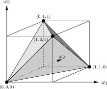
Figure 5: The fundamental polytope for $\mathbf{H}=[1~{}1~{}1]$.

Vectors in $\mathcal{P}(\mathbf{H})$ are called pseudo-codewords of $\mathbf{H}$, and we will call any vector in $\mathcal{K}(\mathbf{H})$ a pseudo-codeword and two pseudo-codewords that are equal up to a positive scaling constant will be considered to be equivalent. Clearly, not all pseudo-codewords are codewords, but all codewords are pseudo-codewords.

The fundamental cone and polytope can both be described by certain sets of inequalities that are computationally useful [3, 16]. Since our study of pseudo-codewords will rely heavily on the fundamental cone, we now describe it in more detail.

A vector $\boldsymbol{\omega}=(\omega_{1},\ldots,\omega_{n})\in\mathbb{R}^{n}$ is in the fundamental cone $\mathcal{K}\triangleq\mathcal{K}(\mathbf{H})$ if and only if

$$\omega_{i}\geq 0\quad \text{for all $i\in\mathcal{I}(\mathbf{H})$},$$ (2.4)

$$\sum_{i\in(\mathcal{I}_{j}\setminus\{i^{\prime}\})}\omega_{i}\geq\omega_{i^{\prime}}\quad \text{for all $j\in\mathcal{J}(\mathbf{H})$ and for all $i^{\prime}\in\mathcal{I}_{j}(\mathbf{H})$}.$$ (2.5)

Example 2.7.

Let $\mathbf{H}\triangleq[1,\ 1,\ 1]$ be a parity-check matrix for the code $\mathsf{C}=\{(0,0,0),\ (1,1,0),$ $(1,0,1),\ (0,1,1)\}$. The fundamental polytope $\mathcal{P}(\mathbf{H})$ associated with $\mathbf{H}$ is (see Fig. 5)

$$\mathcal{P}(\mathbf{H}) =\left\{(\omega_{1},\omega_{2},\omega_{3})\in\mathbb{R}^{3}\left|\begin{array}[]{l}0\leq\omega_{1}\leq 1\\ 0\leq\omega_{2}\leq 1\\ 0\leq\omega_{3}\leq 1\end{array}\quad\begin{array}[]{l}-\omega_{1}+\omega_{2}+\omega_{3}\geq 0\\ +\omega_{1}-\omega_{2}+\omega_{3}\geq 0\\ +\omega_{1}+\omega_{2}-\omega_{3}\geq 0\\ +\omega_{1}+\omega_{2}+\omega_{3}\leq 2\end{array}\right.\right\},$$

from which we obtain the fundamental cone $\mathcal{K}(\mathbf{H})$ associated with $\mathbf{H}$:

$$\mathcal{K}(\mathbf{H}) =\left\{(\omega_{1},\omega_{2},\omega_{3})\in\mathbb{R}^{3}\left|\begin{array}[]{l}0\leq\omega_{1}\\ 0\leq\omega_{2}\\ 0\leq\omega_{3}\end{array}\quad\begin{array}[]{l}-\omega_{1}+\omega_{2}+\omega_{3}\geq 0\\ +\omega_{1}-\omega_{2}+\omega_{3}\geq 0\\ +\omega_{1}+\omega_{2}-\omega_{3}\geq 0\end{array}\right.\right\}.$$

We see that the pseudo-codeword $\boldsymbol{\omega}=\bigl{(}\frac{2}{3},\frac{2}{3},\frac{2}{3}\bigr{)}$ satisfies the inequalities of both the fundamental polytope and the fundamental cone. Also, the pseudo-codeword $\boldsymbol{\omega}=(1,1,1)$ and its positive multiples are in the fundamental cone but not necessarily in the fundamental polytope. $\square$

Remark 2.8.

As explained briefly in Sec. 1, pseudo-codewords can also be described using graph theory language as vectors corresponding to codewords in a cover graph. Looking again at the cover tower $\mathcal{G}\triangleq\mathcal{G}^{(r)}$, $\mathcal{G}^{(2r)}$, $\mathcal{G}^{(4r)}$, $\ldots$, a codeword $\mathbf{c}(D)$ of a larger graph, say $\mathsf{C}_{\mathrm{QC}}^{(4r)}$, seen as a vector with real components, when projected over $\mathbb{R}$ onto the graphs of $\mathsf{C}_{\mathrm{QC}}^{(r)}$ and $\mathsf{C}_{\mathrm{QC}}^{(2r)}$, using the formula $\mathbf{c}(X)\operatorname{mod}\,(X^{r}-1)$, respectively, $\mathbf{c}(X)\operatorname{mod}\,(X^{2r}-1)$, gives a pseudo-codeword. Similarly, a codeword $\mathbf{c}(D)$ of the unwrapped convolutional code $\mathsf{C}_{\mathrm{conv}}$, when projected onto the graphs of $\mathsf{C}_{\mathrm{QC}}^{(r)}$ $\mathsf{C}_{\mathrm{QC}}^{(2r)}$, $\mathsf{C}_{\mathrm{QC}}^{(4r)},\ldots,$ using the formulas $\mathbf{c}(X)\operatorname{mod}\,(X^{r}-1)$, $\mathbf{c}(X)\operatorname{mod}\,(X^{2r}-1)$, $\mathbf{c}(X)\operatorname{mod}\,(X^{4r}-1),\ldots$, gives pseudo-codewords in the QC codes.

Example 2.9.

Let $\overline{\mathbf{c}}\triangleq(1{:}1{:}0,\ 1{:}1{:}0,\ 1{:}1{:}0)\in{\rm Nullsp}(\mathbf{H}_{\mathrm{QC}}^{(3)})$ be the codeword identified in Example 2.5 for the code $\mathsf{C^{(3)}}$, with corresponding polynomial description $\mathbf{c}(X)\triangleq(1+X,1+X,1+X)\in{\rm Nullsp}(\mathbf{H}_{\mathrm{QC}}^{(3)}(X))$. When projecting $\mathbf{c}(X)$ over $\mathbb{R}$ onto the graph of $\mathsf{C}=\{(0,0,0)\}$ we obtain $\mathbf{c}(X)\operatorname{mod}\,(X-1)=(2,2,2)$, which is a pseudo-codeword in $\mathsf{C}$, equivalent to the pseudo-codeword $\boldsymbol{\omega}=\bigl{(}\frac{2}{3},\frac{2}{3},\frac{2}{3}\bigr{)}$ presented in Example 1.1. The fundamental cone of the convolutional code given by $\mathbf{H}_{\mathrm{conv}}(D)$ in Example 2.3 is trivially zero, i.e., it does not contain any non-zero pseudo-codewords.

$\square$

Remark 2.10.

In the above example we made the following important connection between two graphical ways of representing pseudo-codewords $\boldsymbol{\omega}$ of a QC code $\mathsf{C}$ of length $rL$ as vectors corresponding to codewords $\mathbf{c}(X)$ in some QC code (or convolutional code) associated with an $m$-cover (or an infinite cover) of the graph of $\mathsf{C}$. We can see them as vectors with each entry representing an average of the ones attributed to the variable nodes of the cover graph that are in the “cloud” of that entry, e. g., $\boldsymbol{\omega}=\bigl{(}\frac{2}{3},\frac{2}{3},\frac{2}{3}\bigr{)}$, corresponding to pseudo-codewords in the polytope of $\mathsf{C}$, or we can see them as vectors that are the projections of $\mathbf{c}(X)$ onto the code $\mathsf{C}$ by the formula $\mathbf{c}(X)\operatorname{mod}\,(X^{r}-1)$, e.g., $\boldsymbol{\omega}=(2,2,2)$, corresponding to pseudo-codewords in the fundamental cone of $\mathsf{C}$ that are not necessarily in the polytope.

In fact a similar statement can be made about pseudo-codewords in any block code $\mathsf{C}$ of length $rL$, not having necessarily a QC structure. A pseudo-codeword $\boldsymbol{\omega}$ in $\mathsf{C}$ is a vector corresponding to some codeword $\overline{\mathbf{c}}$ in some block code (or convolutional code) associated with an $m$-cover (or an infinite cover) of the graph of $\mathsf{C}$ with each entry representing an average of the ones attributed to the variable nodes of the cover graph that are in the “cloud” of that entry. However, this is the same, under the equivalence between different representations of a pseudo-codeword in the fundamental cone, as defining a pseudo-codeword $\boldsymbol{\omega}$ as a vector for which there exists a cover corresponding to a block code or to a convolutional code, $\overline{\mathsf{C}}$, of the code $\mathsf{C}$, and there exists some codeword, $\overline{\mathbf{c}}$ in $\overline{\mathsf{C}}$, such that $\boldsymbol{\omega}=\tilde{\mathbf{c}}\operatorname{mod}\,(rL)$ where the vector $\tilde{\mathbf{c}}$ is equal to a permutation of the vector $\overline{\mathbf{c}}$ (where the components of $\overline{\mathbf{c}}$ are taken in the following order $1,m+1,\ldots,(L-1)m+1,2,m+2,\ldots,(L-1)m+2,\ldots,m-1,2m-1,\ldots,Lm-1$). The vector $\tilde{\mathbf{c}}$ it is seen as a vector with real entries and the modular operation $\operatorname{mod}\,(rL)$ is performed over the real numbers.

The above description of the fundamental polytope and cone provides computationally easy descriptions of the pseudo-codewords, especially in the case of QC and convolutional codes. From (2.4) and (2.5) it follows that for any parity-check matrix $\mathbf{H}$ there is a matrix $\mathbf{K}$ such that a vector $\boldsymbol{\omega}$ is a pseudo-codeword in the fundamental code $\mathcal{K}(\mathbf{H})$ if and only if $\mathbf{K}\cdot\boldsymbol{\omega}^{\mathsf{T}}\geq\mathbf{0}^{\mathsf{T}}$. In the case of QC and convolutional codes, the fundamental cone can be described with the help of polynomial matrices. Namely, for any $\mathbf{H}_{\mathrm{QC}}^{(r)}(X)$ there is a polynomial matrix $\mathbf{K}_{\mathrm{QC}}^{(r)}(X)$ such that $\boldsymbol{\omega}(X)\in\mathcal{K}\bigl{(}\mathbf{H}_{\mathrm{QC}}^{(r)}(X)\bigr{)}$ if and only if $\mathbf{K}_{\mathrm{QC}}^{(r)}(X)\cdot\boldsymbol{\omega}(X)^{\mathsf{T}}\geq\mathbf{0}^{\mathsf{T}}$. Similarly, for any $\mathbf{H}_{\mathrm{conv}}(D)$ there is a polynomial matrix $\mathbf{K}_{\mathrm{conv}}(D)$ such that $\boldsymbol{\omega}(D)\in\mathcal{K}\bigl{(}\mathbf{H}_{\mathrm{conv}}(D)\bigr{)}$ if and only if $\mathbf{K}_{\mathrm{conv}}(D)\cdot\boldsymbol{\omega}(D)^{\mathsf{T}}\geq\mathbf{0}^{\mathsf{T}}$.

This fundamental-cone description is particularly simple and hence useful in the case of monomial parity-check matrices $\mathbf{H}_{\mathrm{conv}}$ (see [6]), since the fundamental-cone inequalities can then be stated very simply as follows. A vector $\boldsymbol{\omega}$ is a pseudo-codeword in the fundamental cone of a monomial matrix $\mathbf{H_{\rm conv}}$ if and only if the associated polynomial vector $\boldsymbol{\omega}(D)=\bigl{(}\omega_{1}(D),\omega_{2}(D),\ldots,\omega_{L}(D)\bigr{)}$ satisfies:

$$\omega_{\ell}(D)\geq 0, \quad\text{for all $\ell\in\{1,\ldots,L\}$},$$

$$\sum_{\ell\in\{1,\ldots,L\}\setminus\{\ell^{\prime}\}}h_{j\ell}(D)\omega_{\ell}(D)\geq h_{j\ell^{\prime}}(D)\omega_{\ell^{\prime}}(D), \quad\text{for all $j\in\{1,\ldots,J\}$, for all $\ell^{\prime}\in\{1,\ldots,L\}$}.$$

Equivalently, if $\boldsymbol{\Omega}(D)$ is an $L\times L$ matrix with $\ell$-th row vector

$$\begin{pmatrix}+\omega_{1}(D)&\cdots&+\omega_{\ell-1}(D)&-\omega_{\ell}(D)&+\omega_{\ell+1}(D)&\cdots&\omega_{L}(D)\end{pmatrix}$$

for $j\in\{1,\ldots,L\}$, then $\boldsymbol{\omega}(D)$ is a pseudo-codeword if and only if $\boldsymbol{\omega}_{\ell}(D)\geq\mathbf{0}$ for all $\ell\in\{1,\ldots,L\}$ and

$$\mathbf{H}_{\mathrm{conv}}(D)\cdot\boldsymbol{\Omega}(D)^{\mathsf{T}} \geq\mathbf{0}.$$

Example 2.11.

Let

$$\mathbf{H}_{\mathrm{conv}}(D) \triangleq\begin{bmatrix}1&1&1&1\\ 1&D&D^{2}&D^{3}\\ 1&D^{4}&D^{3}&D^{2}\end{bmatrix}$$

be a polynomial parity-check matrix of a rate-$1/4$ convolutional code. The following vector

$$\boldsymbol{\omega}(D) \triangleq\begin{pmatrix}3D^{2}+D^{3}&4D+D^{2}&3+D+4D^{2}+D^{3}&3+4D+D^{2}\end{pmatrix}$$

$$=\begin{pmatrix}0&0&3&3\end{pmatrix}+\begin{pmatrix}0&4&1&4\end{pmatrix}D+\begin{pmatrix}3&1&4&1\end{pmatrix}D^{2}+\begin{pmatrix}1&0&1&0\end{pmatrix}D^{3},$$

corresponding to the scalar vector

$$\overline{\boldsymbol{\omega}} =\left(0,0,3,3,\ 0,4,1,4,\ 3,1,4,1,\ 1,0,1,0,\ \cdots\right),$$

is a pseudo-codeword for the convolutional code since $\boldsymbol{\omega}(D)\geq\mathbf{0}$ and the matrix

$$\boldsymbol{\Omega}(D)\triangleq\begin{bmatrix}-3D^{2}-D^{3}&+4D+D^{2}&+3+D+4D^{2}+D^{3}&+3+4D+D^{2}\\ +3D^{2}+D^{3}&-4D-D^{2}&+3+D+4D^{2}+D^{3}&+3+4D+D^{2}\\ +3D^{2}+D^{3}&+4D+D^{2}&-3-D-4D^{2}-D^{3}&+3+4D+D^{2}\\ +3D^{2}+D^{3}&+4D+D^{2}&+3+D+4D^{2}+D^{3}&-3-4D-D^{2}\end{bmatrix}$$

gives

$$\mathbf{H}_{\mathrm{conv}}(D)\cdot\boldsymbol{\Omega}(D)^{\mathsf{T}} =\begin{bmatrix}6+9D+3D^{2}&4D^{2}+4D^{3}+8D^{4}+2D^{5}&6D^{3}+2D^{4}+8D^{5}+2D^{6}\\ 6+D+D^{2}+2D^{3}&2D^{2}+4D^{3}+8D^{4}+2D^{5}&6D^{2}+8D^{3}+2D^{4}+2D^{6}\\ 7D+D^{2}&4D^{2}+4D^{3}&6D^{2}+2D^{3}\\ D+7D^{2}+2D^{3}&10D^{2}&8D^{5}+2D^{6}\end{bmatrix}^{\mathsf{T}}$$

$$\geq\mathbf{0},$$

i.e., $\mathbf{H}_{\mathrm{conv}}(D)\cdot\boldsymbol{\Omega}(D)^{\mathsf{T}}$ has all polynomial entries with non-negative coefficients. $\square$

Similarly, for a QC code that is described by a monomial $J\times L$ parity-check matrix $\mathbf{H}_{\mathrm{QC}}^{(r)}(X)$, a vector $\boldsymbol{\omega}(X)$ is a pseudo-codeword in the corresponding fundamental cone if and only if the associated polynomial vector $\boldsymbol{\omega}(X)=\bigl{(}\omega_{1}(X),\omega_{2}(X),\ldots,\omega_{L}(X)\bigr{)}$ satisfies

$$\big{(}\omega_{\ell}(X)\operatorname{mod}\,(X^{r}-1)\big{)}\geq 0 \quad\quad\text{for all $\ell\in\{1,\ldots,L\}$},$$

and

$$\left(\mathbf{H}_{\mathrm{QC}}^{(r)}(X)\boldsymbol{\Omega}(X)^{\mathsf{T}}\operatorname{mod}\,(X^{r}-1)\right)\geq\mathbf{0}.$$

Example 2.12.

Let $\mathbf{H}_{\mathrm{QC}}^{(5)}(X)$ be the $r=5$ parity-check matrix obtained from $\mathbf{H}_{\mathrm{conv}}(D)$ in Example 2.11 for a QC block code of length $n=20$. Then, for the polynomial vector

$$\boldsymbol{\omega}^{(5)}(X) \triangleq\begin{pmatrix}3X^{2}+X^{3}&4X+X^{2}&3+X+4X^{2}+X^{3}&3+4X+X^{2}\end{pmatrix},$$

we obtain

$$\mathbf{H}_{\mathrm{QC}}^{(5)}(X)\boldsymbol{\Omega}(X)^{\mathsf{T}}\operatorname{mod}\,(X^{5}-1)$$

$$\quad\quad=\begin{bmatrix}6+9X+3X^{2}&2+4X^{2}+4X^{3}+8X^{4}&8+2X+6X^{3}+2X^{4}\\ 6+X+X^{2}+2X^{3}&2+2X^{2}+4X^{3}+8X^{4}&2X+6X^{2}+8X^{3}+2X^{4}\\ 7X+X^{2}&4X^{2}+4X^{3}&6X^{2}+2X^{3}\\ X+7X^{2}+2X^{3}&10X^{2}&8+2X\end{bmatrix}^{\mathsf{T}}.$$

Since $\boldsymbol{\omega}^{(5)}(X)\geq\mathbf{0}$ and $(\mathbf{H}_{\rm QC}^{(5)}(X)\boldsymbol{\Omega}(X)^{\mathsf{T}}\operatorname{mod}\,(X^{5}-1))\geq\mathbf{0}$, we know that $\boldsymbol{\omega}^{(5)}(X)$ is a pseudo-codeword. $\square$

The pseudo-codeword $\boldsymbol{\omega}(D)=(3D^{2}+D^{3},\ 4D+D^{2},\ 3+D+4D^{2}+D^{3},\ 3+4D+D^{2})$ in Example 2.11 was obtained by using a method to be described in Sec. 4. Projecting this pseudo-codeword in the convolutional code onto the $r$-wrapped QC code, for $r=5$, we obtained the pseudo-codeword $\boldsymbol{\omega}(X)=(3X^{2}+X^{3},\ 4X+X^{2},\ 3+X+4X^{2}+X^{3},\ 3+4X+X^{2})$ in the QC code. This is not a mere coincidence as the following lemma shows.

Lemma 2.13.

Let $\boldsymbol{\omega}(D)$ be a pseudo-codeword in the convolutional code defined by $\mathbf{H}_{\mathrm{conv}}(D)$, i.e., $\boldsymbol{\omega}(D)\in\mathcal{K}(\mathbf{H}_{\mathrm{conv}}(D))$. Then its $r$ wrap-around polynomial vector is a pseudo-codeword in the associated QC-code defined by $\mathbf{H}_{\mathrm{QC}}^{(r)}(X)$, i.e., $\boldsymbol{\omega}(X)\operatorname{mod}\,(X^{r}-1)\in\mathcal{K}(\mathbf{H}_{\mathrm{QC}}^{(r)}(X))$.

Proof: We have seen that for any $\mathbf{H}_{\mathrm{conv}}(D)$ describing a convolutional code there is a matrix $\mathbf{K}_{\mathrm{conv}}(D)$ such that a polynomial vector $\boldsymbol{\omega}(D)$ is a pseudo-codeword in the fundamental cone $\mathcal{K}(\mathbf{H}_{\mathrm{conv}}(D))$ if and only if $\mathbf{K}_{\mathrm{conv}}(D)\boldsymbol{\omega}(D)^{\mathsf{T}}\geq\mathbf{0}^{\mathsf{T}}$. By reducing $\mathbf{K}_{\mathrm{conv}}(D)$ modulo $D^{r}-1$, we obtain a matrix $\mathbf{K}_{\mathrm{QC}}^{(r)}(X)=\left(\mathbf{K}_{\mathrm{conv}}(X)\operatorname{mod}\,(X^{r}-1)\right)$ with the property that a polynomial vector $\boldsymbol{\omega}(X)$ is a pseudo-codeword in the fundamental cone $\mathcal{K}(\mathbf{H}_{\mathrm{QC}}^{(r)}(X))$ if and only if $\mathbf{K}_{\mathrm{QC}}^{(r)}(X)\boldsymbol{\omega}(X)^{\mathsf{T}}\geq\mathbf{0}^{\mathsf{T}}$. Reducing $\mathbf{K}_{\mathrm{conv}}(D)\boldsymbol{\omega}(D)^{\mathsf{T}}\geq\mathbf{0}^{\mathsf{T}}$ modulo $D^{r}-1$, we obtain $\mathbf{K}_{\mathrm{QC}}^{(r)}(X)(\boldsymbol{\omega}(X)\operatorname{mod}\,(X^{r}-1))^{\mathsf{T}}\geq\mathbf{0}^{\mathsf{T}}$, which proves the claim. $\Box$

Remark 2.14.

This result can be easily deduced using the graph-theory language at the end of Sec. 2.1. Indeed, looking again at the cover tower $\mathcal{G}\triangleq\mathcal{G}^{(r)},\mathcal{G}^{(2r)},\mathcal{G}^{(4r)},\ldots$, a pseudo-codeword $\mathbf{\boldsymbol{\omega}}(D)$ of a larger graph, say $\mathsf{C}_{\mathrm{QC}}^{(4r)}$, when projected onto the graphs of $\mathsf{C}_{\mathrm{QC}}^{(r)}$ and $\mathsf{C}_{\mathrm{QC}}^{(2r)}$, using the formula $\mathbf{\boldsymbol{\omega}}(X)\operatorname{mod}\,(X^{r}-1)$, respectively, $\mathbf{\boldsymbol{\omega}}(X)\operatorname{mod}\,(X^{2r}-1)$, gives another pseudo-codeword. Similarly, a pseudo-codeword $\mathbf{\boldsymbol{\omega}}(D)$ of the unwrapped convolutional code $\mathsf{C}_{\mathrm{conv}}$, when projected onto the graphs of $\mathsf{C}_{\mathrm{QC}}^{(r)}$ $\mathsf{C}_{\mathrm{QC}}^{(2r)}$, $\mathsf{C}_{\mathrm{QC}}^{(4r)},\ldots,$ using the formulas $\mathbf{\boldsymbol{\omega}}(X)\operatorname{mod}\,(X^{r}-1)$, $\mathbf{\boldsymbol{\omega}}(X)\operatorname{mod}\,(X^{2r}-1)$, $\mathbf{\boldsymbol{\omega}}(X)\operatorname{mod}\,(X^{4r}-1),\ldots,$ gives pseudo-codewords in the QC codes.

Example 2.15.

The pseudo-codeword

$$\boldsymbol{\omega}(D) \triangleq\begin{pmatrix}3D^{2}+D^{3}&4D+D^{2}&3+D+4D^{2}+D^{3}&3+4D+D^{2}\end{pmatrix}$$

of the convolutional code in Example 2.11 projects onto the following pseudo-codewords in the QC wrapped block code versions of parity-check matrix $\mathbf{H}_{\mathrm{QC}}^{(r)}(X)=\mathbf{H}_{\mathrm{conv}}(X)\operatorname{mod}\,(X^{r}-1)$, for all $r\geq 0$:

$$\boldsymbol{\omega}^{(r)}(X) \triangleq\boldsymbol{\omega}(D)\operatorname{mod}\,(X^{r}-1)=\begin{pmatrix}3X^{2}+X^{3}&4X+X^{2}&3+X+4X^{2}+X^{3}&3+4X+X^{2}\end{pmatrix},$$

$${\rm~{}for~{}all~{}}r\geq 4,~{}(r=5{\rm~{}case~{}above~{}is~{}included},)$$

$$\boldsymbol{\omega}^{(3)}(X) \triangleq\boldsymbol{\omega}(D)\operatorname{mod}\,(X^{3}-1)=\begin{pmatrix}1+3X^{2}&4X+X^{2}&4+X+4X^{2}&3+4X+X^{2}\end{pmatrix},$$

$$\boldsymbol{\omega}^{(2)}(X) \triangleq\boldsymbol{\omega}(D)\operatorname{mod}\,(X^{2}-1)=\begin{pmatrix}3+X&1+4X&7+2X&4+4X\end{pmatrix},$$

$$\boldsymbol{\omega}^{(1)}(X) \triangleq\boldsymbol{\omega}(D)\operatorname{mod}\,(X-1)~{}=\begin{pmatrix}4&5&9&8\end{pmatrix}.$$

$\square$

3 Pseudo-Weight Comparison Between QC Codes and Convolutional Codes

This section begins with an introductory subsection in which various channel pseudo-weights are defined and continues with the main result that the minimum AWGNC, BEC, BSC, and max-fractional pseudo-weights of a convolutional code are at least as large as the corresponding pseudo-weights of a wrapped QC block code.

3.1 Definitions of Channel Pseudo-Weights

Definition 3.1.

​​[2, 3, 16, 15, 4, 5] Let $\boldsymbol{\omega}=(\omega_{0},$ $\ldots,\omega_{n-1})$ be a nonzero vector in $\mathbb{R}_{+}^{n}$. The AWGNC pseudo-weight and the BEC pseudo-weight of the vector $\boldsymbol{\omega}$ are defined to be, respectively,

$$w_{\mathrm{p}}^{\mathrm{AWGNC}}(\boldsymbol{\omega}) \triangleq\frac{\lVert\boldsymbol{\omega}\rVert_{1}^{2}}{\lVert\boldsymbol{\omega}\rVert_{2}^{2}},\quad\quad w_{\mathrm{p}}^{\mathrm{BEC}}(\boldsymbol{\omega})=\big{|}\operatorname{supp}(\boldsymbol{\omega})\big{|},$$

where $\lVert\boldsymbol{\omega}\rVert_{1}$ and $\lVert\boldsymbol{\omega}\rVert_{2}$ are the $1$-norm, respectively $2$-norm, of $\boldsymbol{\omega}$, and $\operatorname{supp}(\boldsymbol{\omega})$ is the set of all indices $i$ corresponding to nonzero components $\omega_{i}$ of $\boldsymbol{\omega}$. In order to define the BSC pseudo-weight $w_{\mathrm{p}}^{\mathrm{BSC}}(\boldsymbol{\omega})$, we let $\boldsymbol{\omega}^{\prime}$ be the vector of length $n$ with the same components as $\boldsymbol{\omega}$ but in non-increasing order. Now let

$$f(\xi) \triangleq\omega^{\prime}_{i}\quad(i<\xi\leq i+1,\ 0<\xi\leq n),\quad\quad F(\xi)\triangleq\int_{0}^{\xi}f(\xi^{\prime})\,\operatorname{d}{\xi^{\prime}},\quad\text{ and }\quad e\triangleq F^{-1}\left(\frac{F(n)}{2}\right).$$

Then the binary symmetric channel (BSC)-pseudo-weight $w_{\mathrm{p}}^{\mathrm{BSC}}(\boldsymbol{\omega})$ is $w_{\mathrm{p}}^{\mathrm{BSC}}(\boldsymbol{\omega})\triangleq 2e$. Finally, the fractional weight of a vector $\boldsymbol{\omega}\in[0,1]^{n}$ and the max-fractional weights of a vector $\boldsymbol{\omega}\in\mathbb{R}_{+}^{n}$ are defined to be, respectively,

$$w_{\mathrm{frac}}(\boldsymbol{\omega}) =\lVert\boldsymbol{\omega}\rVert_{1},\quad\quad w_{\mathrm{max-frac}}(\boldsymbol{\omega})\triangleq\frac{\lVert\boldsymbol{\omega}\rVert_{1}}{\lVert\boldsymbol{\omega}\rVert_{\infty}},$$

where $\lVert\boldsymbol{\omega}\rVert_{\infty}$ is the infinite or max norm. For $\boldsymbol{\omega}=\mathbf{0}$ we define all of the above pseudo-weights, fractional weights, and max-fractional weights to be zero. $\square$

A discussion of the motivation and significance of these definitions can be found in [3]. Note that whereas the fractional weight has an operational meaning only for vertices of the fundamental polytope, the other measures have an operational meaning for any vector in the fundamental polytope or cone. Note also that here $w_{\mathrm{frac}}$ and $w_{\mathrm{max-frac}}$ are defined for any vector in $\mathbb{R}_{+}^{n}$, whereas $w_{\mathrm{frac}}$ and $w_{\mathrm{max-frac}}$ in [15] are what we will call $w^{\mathrm{min}}_{\mathrm{frac}}$ and $w^{\mathrm{min}}_{\mathrm{max-frac}}$.

Example 3.2.

Let

$$\boldsymbol{\omega}(D) =\begin{pmatrix}3D^{2}+D^{3}&4D+D^{2}&3+D+4D^{2}+D^{3}&3+4D+D^{2}\end{pmatrix}$$

be the pseudo-codeword in Example 2.11 and let $\overline{\boldsymbol{\omega}}=(0,0,3,3,\ 0,4,1,4,\ 3,1,4,1,\ 1,0,1,0,\$ $0,0,0,0,\ \ldots)$ be its scalar vector description. Then

$$w_{\mathrm{p}}^{\mathrm{AWGNC}}(\boldsymbol{\omega}) =\frac{\lVert\boldsymbol{\omega}\rVert_{1}^{2}}{\lVert\boldsymbol{\omega}\rVert_{2}^{2}}=\frac{(3\cdot 4+3\cdot 3+5\cdot 1)^{2}}{3\cdot 16+3\cdot 9+5\cdot 1}=8.45,\quad\quad w_{\mathrm{p}}^{\mathrm{BEC}}(\boldsymbol{\omega})=|\operatorname{supp}(\boldsymbol{\omega})|=11.$$

In order to compute $w_{\mathrm{p}}^{\mathrm{BSC}}(\boldsymbol{\omega})$, we let $\overline{\boldsymbol{\omega}}^{\prime}=(4,4,4,3,3,3,1,1,1,1,1,0,0,0,0,0,\ldots)$ be the vector that lists the components of $\boldsymbol{\omega}$ in non-increasing order. We obtain $w_{\mathrm{p}}^{\mathrm{BSC}}(\boldsymbol{\omega})=2e=\frac{20}{3}=6.67$, since we need to add up $e=\frac{10}{3}$ ordered components of $\boldsymbol{\omega}^{\prime}$ to obtain $\frac{\lVert\boldsymbol{\omega}\rVert_{1}}{2}=13$. Finally $\lVert\boldsymbol{\omega}\rVert_{\infty}=\max_{i=1}^{16}\omega_{i}$, from which it follows that $w_{\mathrm{max-frac}}(\boldsymbol{\omega})=\frac{\lVert\boldsymbol{\omega}\rVert_{1}}{\lVert\boldsymbol{\omega}\rVert_{\infty}}=\frac{26}{4}=6.5$. $\square$

A measure of the effect that the pseudo-codewords have on the performance of a code is given by the minimum pseudo-weight [2, 3, 15, 16]

$$w_{\mathrm{p}}^{\mathrm{min}}(\mathbf{H}) \triangleq\min_{\boldsymbol{\omega}\in\mathcal{V}(\mathcal{P}(\mathbf{H}))\setminus\{\mathbf{0}\}}w_{\mathrm{p}}(\boldsymbol{\omega}),$$

where $\mathcal{V}(\mathcal{P}(\mathbf{H}))\setminus\{\mathbf{0}\}$ is the set of all non-zero vertices in the fundamental polytope $\mathcal{P}(\mathbf{H})$ and the pseudo-weights are the appropriate ones for each channel (AWGNC, BSC, and BEC pseudo-weights) and the minimum fractional and max-fractional weights.

Computing these values can be quite challenging, since the task of finding the set of vertices of $\mathcal{P}(\mathbf{H})$ is in general very complex. However, in the case of four of the above pseudo-weights (the minimum AWGNC, BSC, and BEC pseudo-weights and the minimum max-fractional weight) there is a computationally simpler description given by

$$w_{\mathrm{p}}^{\mathrm{min}}(\mathbf{H}) =\min_{\boldsymbol{\omega}\in\mathcal{K}(\mathbf{H})\setminus\{\mathbf{0}\}}w_{\mathrm{p}}(\boldsymbol{\omega}),$$

for the appropriate pseudo-weight. (Note that there is no such statement for the minimum fractional weight; see, e.g., [16, 3]).

Example 3.3.

Let $\mathbf{H}_{\mathrm{QC}}^{(5)}(X)$ be the matrix of Example 2.12 and let $\mathsf{C}_{\mathrm{QC}}^{(r)}$ be the QC block code of length $n=20$, with $r=5$. The minimum distance is 6 and it is equal to the $w_{\mathrm{p}}^{\mathrm{AWGNC,min}}(\mathbf{H}_{\rm QC}^{(5)})$. (This was obtained using a vertex enumeration program for polytopes that lists all the minimal pseudo-codewords of a code, see [21].) $\square$

Remark 3.4.

In [3] it was shown that for any code defined by a parity-check matrix $\mathbf{H}$, the following inequalities hold:

$$w^{\mathrm{min}}_{\mathrm{frac}}(\mathbf{H}) \leq w^{\mathrm{min}}_{\mathrm{max-frac}}(\mathbf{H}) \leq w_{\mathrm{p}}^{\mathrm{AWGNC,min}}(\mathbf{H}) \leq w_{\mathrm{p}}^{\mathrm{BEC,min}}(\mathbf{H}),$$

$$w^{\mathrm{min}}_{\mathrm{frac}}(\mathbf{H}) \leq w^{\mathrm{min}}_{\mathrm{max-frac}}(\mathbf{H}) \leq w_{\mathrm{p}}^{\mathrm{BSC,min}}(\mathbf{H}) \leq w_{\mathrm{p}}^{\mathrm{BEC,min}}(\mathbf{H}).$$

Therefore, $w^{\mathrm{min}}_{\mathrm{frac}}(\mathbf{H})$ and $w^{\mathrm{min}}_{\mathrm{max-frac}}(\mathbf{H})$ can serve as lower bounds for $w_{\mathrm{p}}^{\mathrm{AWGNC,min}}(\mathbf{H})$, $w_{\mathrm{p}}^{\mathrm{BSC,min}}(\mathbf{H})$, and $w_{\mathrm{p}}^{\mathrm{BEC,min}}(\mathbf{H})$.

3.2 Minimum Pseudo-Weights

In what follows, we compare the minimum pseudo-weights and minimum max-fractional weight of a QC block code to those of its corresponding convolutional code which we assume to have a fundamental cone containing non-zero vectors. In order to analyze the minimum pseudo-weight and minimum max-fractional weight, it is sufficient to analyze the weights of the non-zero vectors in the fundamental cone. Throughout this section, without loss of generality, all pseudo-codewords $\boldsymbol{\omega}(D)$ are assumed to have finite support.

Theorem 3.5.

For the AWGNC, BEC, and BSC pseudo-weights, if $\boldsymbol{\omega}(D)\in\mathcal{K}(\mathbf{H}_{\mathrm{conv}}(D))$, then

$$w_{\mathrm{p}}\big{(}\boldsymbol{\omega}(X)\operatorname{mod}\,(X^{r}-1)\big{)} \leq w_{\mathrm{p}}\big{(}\boldsymbol{\omega}(D)\big{)}.$$

Therefore, if the fundamental cone of the convolutional code is not trivial (i.e., it contains non-zero vectors) we obtain

$$w_{\mathrm{p}}^{\mathrm{min}}\left(\mathbf{H}_{\mathrm{QC}}^{(r)}(X)\right) \leq w_{\mathrm{p}}^{\mathrm{min}}\big{(}\mathbf{H}_{\mathrm{conv}}(D)\big{)}.$$

Proof: In the following, we need to analyze separately the AWGNC, BEC, and BSC pseudo-weights of $\boldsymbol{\omega}(D)$ and of its $r$ wrap-around $\boldsymbol{\omega}(X)\operatorname{mod}\,(X^{r}-1)$. Let $\boldsymbol{\omega}(D)=\bigl{(}\omega_{1}(D),\ldots,\omega_{L}(D)\bigr{)}$ be a pseudo-codeword. By assumption $\boldsymbol{\omega}(D)$ has finite support, i.e., there exists an integer $t$ such that the maximal degree of any $\omega_{\ell}(D)$, $\ell\in\{1,\ldots,L\}$, is smaller than $t$.

Case 1 (AWGNC): Since $\lVert\boldsymbol{\omega}(D)\rVert_{1}=\lVert\boldsymbol{\omega}(X)\operatorname{mod}\,(X^{r}-1)\rVert_{1}$ and

$$\big{\lVert}\boldsymbol{\omega}(X)\operatorname{mod}\,(X^{r}-1)\big{\rVert}_{2}^{2} =\sum_{\ell=1}^{L}\sum_{i=0}^{r-1}\left(\sum_{i^{\prime}=0}^{\lfloor(t-1)/r\rfloor}\omega_{\ell,i+i^{\prime}r}\right)^{2}\geq\sum_{\ell=1}^{L}\sum_{i=0}^{r-1}\sum_{i^{\prime}=0}^{\lfloor(t-1)/r\rfloor}\omega_{\ell,i+i^{\prime}r}^{2}=\big{\lVert}\boldsymbol{\omega}(D)\big{\rVert}_{2}^{2},$$

we obtain $w_{\mathrm{p}}^{\mathrm{AWGNC}}(\boldsymbol{\omega}(D))\geq w_{\mathrm{p}}^{\mathrm{AWGNC}}(\boldsymbol{\omega}(X)\operatorname{mod}\,(X^{r}-1))$.

Case 2 (BEC): Since the components of the vector $\boldsymbol{\omega}(X)\operatorname{mod}\,(X^{r}-1)$ are obtained by adding in $\mathbb{R}_{+}$ certain non-negative components of $\boldsymbol{\omega}(D)$, it follows that

$$|\operatorname{supp}\boldsymbol{\omega}(D)| \geq|\operatorname{supp}\left(\boldsymbol{\omega}(X)\operatorname{mod}\,(X^{r}-1)\right)|$$

and we obtain $w_{\mathrm{p}}^{\mathrm{BEC}}\big{(}\boldsymbol{\omega}(D)\big{)}\geq w_{\mathrm{p}}^{\mathrm{BEC}}\big{(}\boldsymbol{\omega}(X)\operatorname{mod}\,(X^{r}-1)\big{)}$.

Case 3 (BSC): In order to compare the BSC-pseudo-weight of the two vectors, we first need to arrange the components in decreasing order. Let $M_{0}\geq M_{1}\geq\ldots\geq M_{tL-1}$ and $m_{0}\geq m_{1}\geq\ldots\geq m_{rL-1}$ be listings of all the coefficients of all the components of $\boldsymbol{\omega}(D)$ and $\boldsymbol{\omega}(X)\operatorname{mod}\,(X^{r}-1)$, respectively, in non-increasing order. Since $\lVert\boldsymbol{\omega}(D)\rVert_{1}=\lVert\boldsymbol{\omega}(X)\operatorname{mod}\,(X^{r}-1)\rVert_{1}$, we obtain that $\frac{\lVert\boldsymbol{\omega}(D)\rVert_{1}}{2}=\frac{\lVert\boldsymbol{\omega}(X)\operatorname{mod}\,(X^{r}-1)\rVert_{1}}{2}\triangleq M$, which gives $\sum_{i=0}^{tL-1}M_{i}=\sum_{i=0}^{rL-1}m_{i}=2M$. Hence the two sequences of non-negative integers form two partitions, $\lambda$ and $\mu$, respectively, of $2M$. We fill the shorter partition with zeros so that both partitions have the same length, say $P$. It is enough to show that $\sum_{i=0}^{i^{\prime}-1}M_{i}\leq\sum_{i=0}^{i^{\prime}-1}m_{i}$ for all $i^{\prime}=1,2,\ldots,P$, i.e., that $\mu$ majorizes $\lambda$ [19].

We show first that $m_{0}\geq M_{0}$. Suppose the contrary, i.e., $m_{0}<M_{0}$. Since $m_{i}\leq m_{0}$ for all $i\in\{0,\ldots,P-1\}$, we obtain that $m_{i}<M_{0}$ for all $i\in\{0,\ldots,P-1\}$. But $m_{i}$, $i\in\{0,\ldots,P-1\}$, was obtained by adding over $\mathbb{R}_{+}$ a certain subset of the set $\bigl{\{}M_{i^{\prime}}\ |\ i^{\prime}\in\{0,\ldots P-1\}\bigr{\}}$. So there should be at least one $m_{i^{\prime\prime}}$ that has $M_{0}$ in its composition, and hence $m_{i^{\prime\prime}}\geq M_{0}$. This is a contradiction, from which we obtain $m_{0}\geq M_{0}$.

We finish the proof by induction. Namely, we want to show that from $\sum_{i=0}^{i^{\prime}-1}M_{i}\leq\sum_{i=0}^{i^{\prime}-1}m_{i}$ for some $i^{\prime}\in\{1,\ldots P-1\}$, it follows that $\sum_{i=0}^{i^{\prime}}M_{i}\leq\sum_{i=0}^{i^{\prime}}m_{i}$. If $M_{i^{\prime}}\leq m_{i^{\prime}}$ then this induction step clearly holds. So, assume that $M_{i^{\prime}}>m_{i^{\prime}}$. Since $m_{P-1}\leq\ldots\leq m_{i^{\prime}}<M_{i^{\prime}}\leq M_{i^{\prime}-1}\leq\ldots\leq M_{0}$, we can deduce that $m_{i^{\prime}}$, and in fact all $m_{i}$ with $i^{\prime}\leq i\leq P-1$, cannot contain any $M_{i}$ with $0\leq i\leq i^{\prime}$ in its composition. Hence all possible $M_{i}$, $0\leq i\leq i^{\prime}$, have occurred in the composition of $m_{i}$ for $0\leq i\leq i^{\prime}-1$, which gives $\sum_{i=0}^{i^{\prime}}m_{i}\geq\sum_{i=0}^{i^{\prime}-1}m_{i}\geq\sum_{i=0}^{i^{\prime}}M_{i}$. This proves that $\mu$ majorizes $\lambda$ and we obtain

$$w_{\mathrm{p}}^{\mathrm{BSC}}\big{(}\boldsymbol{\omega}(D)\big{)} \geq w_{\mathrm{p}}^{\mathrm{BSC}}\big{(}\boldsymbol{\omega}(X)\operatorname{mod}\,(X^{r}-1)\big{)}.$$

$\Box$

Theorem 3.5 implies that low-pseudo-weight vectors in the block code may correspond to higher pseudo-weight vectors in the convolutional code, but the opposite is not possible. This suggests that the pseudo-codewords in the block code that result in decoding failures may not cause such failures in the convolutional code, thereby resulting in improved performance for the convolutional code at low-to-moderate signal-to-noise ratios (SNRs).

A similar bound also holds for the max-fractional weight, as shown in the next theorem.

Theorem 3.6.

If $\boldsymbol{\omega}(D)\in\mathcal{K}(\mathbf{H}_{\mathrm{conv}}(D))$, then

$$w_{\mathrm{max-frac}}\big{(}\boldsymbol{\omega}(X)\operatorname{mod}\,(X^{r}-1)\big{)} \leq w_{\mathrm{max-frac}}(\boldsymbol{\omega}(D)).$$

Therefore,

$$w^{\mathrm{min}}_{\mathrm{max-frac}}\left(\mathbf{H}_{\mathrm{QC}}^{(r)}(X)\right) \leq w^{\mathrm{min}}_{\mathrm{max-frac}}\big{(}\mathbf{H}_{\mathrm{conv}}(D)\big{)}.$$

Proof: We have $\lVert\boldsymbol{\omega}(D)\rVert_{1}=\lVert\boldsymbol{\omega}(X)\operatorname{mod}\,(X^{r}-1)\rVert_{1}$ and

$$\big{\lVert}\boldsymbol{\omega}(X)\operatorname{mod}\,(X^{r}-1)\big{\rVert}_{\infty} =\max_{\ell=1}^{L}~{}\max_{i=0}^{r-1}~{}\sum_{i^{\prime}=0}^{\lfloor(t-1)/r\rfloor}\omega_{\ell,i+i^{\prime}r}\geq\max_{\ell=1}^{L}~{}\max_{i=0}^{r-1}~{}\max_{i^{\prime}=0}^{\lfloor(t-1)/r\rfloor}\omega_{\ell,i+i^{\prime}r}\geq\big{\lVert}\boldsymbol{\omega}(D)\big{\rVert}_{\infty},$$

which leads to $w_{\mathrm{max-frac}}(\boldsymbol{\omega}(X)\operatorname{mod}\,(X^{r}-1))\leq w_{\mathrm{max-frac}}(\boldsymbol{\omega}(D)).$ It now follows that

$$w^{\mathrm{min}}_{\mathrm{max-frac}}(\mathbf{H}_{\mathrm{QC}}^{(\mathrm{r})})\leq w^{\mathrm{min}}_{\mathrm{max-frac}}(\mathbf{H}_{\mathrm{conv}}).$$

$\Box$

In the case of the fractional weight, it is easy to see that for any $\boldsymbol{\omega}(D)\in\mathcal{V}(\mathcal{P}(\mathbf{H}_{\mathrm{conv}}(D)))\setminus\{\mathbf{0}\}$, we have $\lVert\boldsymbol{\omega}(D)\rVert_{1}=\lVert\boldsymbol{\omega}(X)\operatorname{mod}\,(X^{r}-1)\rVert_{1}$, and hence $w_{\mathrm{frac}}(\boldsymbol{\omega}(X)\operatorname{mod}\,(X^{r}-1))=w_{\mathrm{frac}}(\boldsymbol{\omega}(D))$. When comparing the minimum fractional weight of the convolutional and QC codes, we encounter a computatinally harder case, as these values must be computed over the set of nonzero pseudo-codewords that are vertices of the fundamental polytope. This is not an easy task, because a vertex pseudo-codeword in the convolutional code might not map into a vertex pseudo-codeword in the QC code.

The theorem below, however, can be established. For its better understanding, we recall that $w^{\mathrm{min}}_{\mathrm{frac}}(\mathbf{H}_{\mathrm{QC}}^{(r)})$ has the following meaning [15, 16]. Let $\mathcal{E}_{\mathrm{QC}}^{(r)}\subseteq{\mathcal{I}}(\mathbf{H}_{\mathrm{QC}}^{(r)})$ be the set of positions where bit flips occurred when using $\mathsf{C}_{\mathrm{QC}}^{(r)}$ for data transmission over a BSC with crossover probability $p$, $0\leq p<1/2$. If $|\mathcal{E}_{\mathrm{QC}}^{(r)}|<\frac{1}{2}w^{\mathrm{min}}_{\mathrm{frac}}(\mathbf{H}_{\mathrm{QC}}^{(r)})$, then LP decoding is correct. Similarly, $w^{\mathrm{min}}_{\mathrm{frac}}(\mathbf{H}_{\mathrm{conv}})$ implies the following. If $\mathcal{E}_{\mathrm{conv}}\subseteq{\mathcal{I}}(\mathbf{H}_{\mathrm{conv}})$ is the set of positions where bit flips occurred when using $\mathsf{C}_{\mathrm{conv}}$ for data transmission over a BSC, then $|\mathcal{E}_{\mathrm{conv}}|<\frac{1}{2}w^{\mathrm{min}}_{\mathrm{frac}}(\mathbf{H}_{\mathrm{conv}})$ guarantees that LP decoding is correct.

Theorem 3.7.

Assume that we are using $\mathsf{C}_{\mathrm{conv}}$ for data transmission over a BSC with cross-over probability $p$, where $0\leq p<1/2$, and that bit flips occur at positions $\mathcal{E}_{\mathrm{conv}}\subseteq{\mathcal{I}}(\mathbf{H}_{\mathrm{conv}})$. If $|\mathcal{E}_{\mathrm{conv}}|<\frac{1}{2}w^{\mathrm{min}}_{\mathrm{frac}}(\mathbf{H}_{\mathrm{QC}}^{(r)})$, then LP decoding is correct. (Note that on the right-hand side of the previous inequality we have $w^{\mathrm{min}}_{\mathrm{frac}}(\mathbf{H}_{\mathrm{QC}}^{(r)})$ and not $w^{\mathrm{min}}_{\mathrm{frac}}(\mathbf{H}_{\mathrm{conv}})$.)

Proof: We know that

$$w^{\mathrm{min}}_{\mathrm{frac}}\left(\mathbf{H}_{\mathrm{QC}}^{(r)}\right) \overset{(*)}{\leq}w^{\mathrm{min}}_{\mathrm{max-frac}}\left(\mathbf{H}_{\mathrm{QC}}^{(r)}\right)\overset{(**)}{\leq}w^{\mathrm{min}}_{\mathrm{max-frac}}\left(\mathbf{H}_{\mathrm{conv}}\right),$$ (3.1)

where step $(*)$ follows from  [15, 16] (see also [3]) and step $(**)$ follows from Theorem 3.6.

Remember that $w^{\mathrm{min}}_{\mathrm{max-frac}}(\mathbf{H}_{\mathrm{QC}}^{(r)})$ has the following meaning [15, 16]. Let $\mathcal{E}_{\mathrm{conv}}\subseteq{\mathcal{I}}(\mathbf{H}_{\mathrm{conv}})$ be the set of positions where the bit flips occured when using $\mathsf{C}_{\mathrm{conv}}$ for data transmission over a BSC. If $|\mathcal{E}_{\mathrm{conv}}|<\frac{1}{2}w^{\mathrm{min}}_{\mathrm{max-frac}}(\mathbf{H}_{\mathrm{conv}})$, then LP decoding is correct.

Now, because the theorem statement assumes that $|\mathcal{E}_{\mathrm{conv}}|<\frac{1}{2}w^{\mathrm{min}}_{\mathrm{frac}}(\mathbf{H}_{\mathrm{QC}}^{(r)})$, using (3.1) we have $|\mathcal{E}_{\mathrm{conv}}|<\frac{1}{2}w^{\mathrm{min}}_{\mathrm{max-frac}}(\mathbf{H}_{\mathrm{conv}})$ and so, according to the meaning of $w^{\mathrm{min}}_{\mathrm{max-frac}}(\mathbf{H}_{\mathrm{conv}})$, LP decoding is correct. $\Box$

Table 1: The pseudo-weights of the pseudo-codewords in Example 2.15.

	$w_{\mathrm{p}}^{\mathrm{AWGNC}}$	$w_{\mathrm{p}}^{\mathrm{BEC}}$	$w_{\mathrm{p}}^{\mathrm{BSC}}$	$w_{\mathrm{max-frac}}$	$w_{\mathrm{frac}}$
$\boldsymbol{\omega}(D)$	$8.45$	$11$	$6.67$	$6.5$	$26$
$\boldsymbol{\omega}(X)\operatorname{mod}\,(X^{r}-1)$
for  all $r\geq 4$	$8.45$	$11$	$6.67$	$6.5$	$26$
$\boldsymbol{\omega}(X)\operatorname{mod}\,(X^{3}-1)$	$7.86$	$10$	$6.5$	$6.5$	$26$
$\boldsymbol{\omega}(X)\operatorname{mod}\,(X^{2}-1)$	$6.09$	$8$	$5$	$3.71$	$26$
$\boldsymbol{\omega}(X)\operatorname{mod}\,(X-1)$	$3.63$	$4$	$3$	$2.89$	$26$

Remark 3.8.

As discussed at the end of Sec. 6 in [3], $w^{\mathrm{min}}_{\mathrm{frac}}(\mathbf{H})$ and $w^{\mathrm{min}}_{\mathrm{max-frac}}(\mathbf{H})$ can give, especially for long codes, quite conservative lower bounds on $w_{\mathrm{p}}^{\mathrm{BSC,min}}(\mathbf{H})$. (E.g., the guarantees on the error correction capabilities of the LP decoder implied by $w^{\mathrm{min}}_{\mathrm{frac}}(\mathbf{H})$ and $w^{\mathrm{min}}_{\mathrm{max-frac}}(\mathbf{H})$ are not good enough to prove the results in [20].) However, a positive fact about $w^{\mathrm{min}}_{\mathrm{frac}}(\mathbf{H})$ and $w^{\mathrm{min}}_{\mathrm{max-frac}}(\mathbf{H})$ is that there are polynomial-time algorithms that compute these two quantities [15, 16].

Remark 3.9.

It is not difficult to adapt Theorem 3.5and Theorem 3.6 such that conclusions similar to the ones in Theorems 3.5 and 3.6 can be drawn with respect to a QC block code with the same structure but a larger circulant size that is a multiple of $r$. In fact, most QC block codes with the same structure but a larger circulant size, even if not a multiple of $r$, behave according to Theorem 3.5. Using similar arguments to the ones in the proofs of these thorems we obtain the following more general inequalities that hold for the AWGNC, BEC, BSC max-fractional and fractional pseudo-weights. If $\boldsymbol{\omega}(D)\in\mathcal{K}(\mathbf{H}_{\mathrm{conv}}(D))$, then

$$w_{\mathrm{p}}\big{(}\boldsymbol{\omega}(X)\operatorname{mod}\,(X^{r}-1)\big{)}\leq w_{\mathrm{p}}\big{(}\boldsymbol{\omega}(X)\operatorname{mod}\,(X^{2r}-1)\big{)}\leq w_{\mathrm{p}}\big{(}\boldsymbol{\omega}(X)\operatorname{mod}\,(X^{4r}-1)\big{)}\leq\ldots\leq w_{\mathrm{p}}\big{(}\boldsymbol{\omega}(D)\big{)},$$

for all $r\geq 1$. In addition, for the AWGNC, BEC, BSC and max-fractional minimum pseudo-weights the following holds for any $m\geq 1$:

$$w_{\mathrm{p}}\big{(}\boldsymbol{\omega}(X)\operatorname{mod}\,(X^{r}-1)\big{)} \leq w_{\mathrm{p}}\big{(}\boldsymbol{\omega}(X)\operatorname{mod}\,(X^{mr}-1)\big{)}.$$

Example 3.10.

To illustrate how the pseudo-weights of the pseudo-codeword in the convolutional code and its projections onto the QC versions satisfy the pseudo-weight inequalities in Remark 3.9 for all the defined pseudo-weights $w_{\mathrm{p}}^{\mathrm{AWGNC}},w_{\mathrm{p}}^{\mathrm{BEC}},w_{\mathrm{p}}^{\mathrm{BSC}},w_{\mathrm{max-frac}}$ and $w_{\mathrm{frac}}$, we computed the pseudo-weights of the pseudo-codewords in Example 2.15. Table 1 contains these results.

$\square$

Next we exemplify some of the bounds on the minimum pseudo-weight of codes proved in this section. We take a tower of three QC codes together with their convolutional version and compute their minimum pseudo-weights which, according to the bounds derived above, form a sequence of increasing numbers, upper bounded by the minimum pseudo-weight of the convolutional version. However, due to the large code parameters, we were able to compute only the minimum pseudo-weight of the smaller code of length 20. For the other QC codes we used the methods of [2, 3] to give lower and upper bounds.

Example 3.11.

Consider the $(3,4)$-regular QC-LDPC code of length $4r$ given by the scalar parity-check matrix, or polynomial parity check matrix, respectively,

$$\mathbf{H}_{\mathrm{QC}}^{(r)} =\begin{bmatrix}\mathbf{I}_{0}&\mathbf{I}_{0}&\mathbf{I}_{0}&\mathbf{I}_{0}\\ \mathbf{I}_{0}&\mathbf{I}_{1}&\mathbf{I}_{2}&\mathbf{I}_{3}\\ \mathbf{I}_{0}&\mathbf{I}_{4}&\mathbf{I}_{3}&\mathbf{I}_{2}\end{bmatrix},\quad\quad\mathbf{H}_{\mathrm{QC}}^{(r)}(X)=\begin{bmatrix}1&1&1&1\\ 1&X&X^{2}&X^{3}\\ 1&X^{4}&X^{3}&X^{2}\end{bmatrix}.$$

Figure 6: The performance of a rate $R=1/4$ $(3,4)$-regular LDPC convolutional code and three associated $(3,4)$-regular QC-LDPC block codes. Note that the horizontal axis is $E_{\mathrm{s}}/N_{0}$ and not the more common $E_{\mathrm{b}}/N_{0}=(1/R)\cdot E_{\mathrm{s}}/N_{0}$.

For $r=5$ we obtain a $[20,7,6]$ code with rate $R=0.35$. By increasing $r$ we obtain other QC codes. By taking powers of $r$ we obtain a tower of QC codes whose graphs form a sequence of covers over the Tanner graph of the $[20,7,6]$ code. For $r\geq 9$, all the codes have minimum distance 10, and hence the free distance of the associated rate $R=1/4$ convolutional code is $d_{\mathrm{free}}=10$, strictly larger than the minimum distance 6 of the $[20,7,6]$ code.

For comparison we simulated these codes together with the associated convolutional code. The results for an AWGN channel are given in Fig. 6. For the $[20,7,6]$ code we ran a vertex enumeration program [21] for polytopes that lists all the minimal pseudo-codewords and found that the minimum pseudo-weight of the $[20,7,6]$ code is $w_{\mathrm{p}}^{\mathrm{AWGNC,min}}=6.00$. The larger parameters of the other three codes allowed us to only lower and upper bound the minimum pseudo-weights. For the $[40,12,10]$ QC code, we have $6.05\leq w_{\mathrm{p}}^{\mathrm{AWGNC,min}}\leq 9.09$ and for the $[80,22,10]$ and the $[160,42,10]$ codes, we obtained the bounds: $6.20\leq w_{\mathrm{p}}^{\mathrm{AWGNC,min}}\leq 9.09$. The slight increase in the lower bound from 6, which is the minimum weight of the $[20,7,6]$ code, to $6.05$ and $6.20$ shows that the minimum AWGNC pseudo-weight of the $[20,7,6]$ code is less than that of the $[40,12,10]$, $[80,22,10]$, and $[160,42,10]$ codes. The slight increase in the lower bounds from $6.05$ to $6.20$ only suggests, but unfortunately gives no further evidence of, the existece of an increasing sequence of minimum AWGNC pseudo-weights for these codes, according to the results of this section.

For completeness, we mention that the techniques in [15, 16] allow us to efficiently compute the minimum max-fractional weight for the above-mentioned codes: we obtain $w^{\mathrm{min}}_{\mathrm{max-frac}}=4.67$ for the length-$20$ code, $w^{\mathrm{min}}_{\mathrm{max-frac}}=5.31$ for the length-$40$ code, $w^{\mathrm{min}}_{\mathrm{max-frac}}=5.33$ for the length-$80$ code, and $w^{\mathrm{min}}_{\mathrm{max-frac}}=5.33$ for the length-$160$ code. Applying the results that were mentioned in Remark 3.4, we see that these values yield weaker lower bounds on $w_{\mathrm{p}}^{\mathrm{AWGNC,min}}$ than the ones given in the previous paragraph.

Using the same vertex enumeration program [21] we could compute as well the minimum pseudo-weights of the QC codes of length $4r$ given by the parity-check matrix $\mathbf{H}_{\mathrm{QC}}^{(r)}(X)$ in Example 3.11 for $r=1,2,3,4$. We present the results in Table 2.

Table 2: The minimum pseudo-weights of the codes $\mathsf{C}_{\mathrm{QC}}^{(r)}$, given by the parity-check matrix $\mathbf{H}_{\mathrm{QC}}^{(r)}(X)$, for $r=1,2,3,4.$

$w_{\mathrm{p}}^{\mathrm{min}}(\mathsf{C}_{\mathrm{QC}}^{(r)})$	$w_{\mathrm{p}}^{\mathrm{AWGNC,min}}$	$w_{\mathrm{p}}^{\mathrm{BEC,min}}$	$w_{\mathrm{p}}^{\mathrm{BSC,min}}$	$w^{\mathrm{min}}_{\mathrm{max-frac}}$
$r=1$	$2$	$2$	$2$	$2$
$r=2$	$2$	$2$	$2$	$2$
$r=3$	$4$	$4$	$4$	$3$
$r=4$	$4$	$4$	$4$	$4$

$\square$

4 Analysis of Problematic Pseudo-Codewords in Convolutional Codes

Studying pseudo-codewords of small pseudo-weight, and, in particular (since the minimum pseudo-weight is upper bounded by the minimum Hamming weight), studying pseudo-codewords of pseudo-weight smaller than the minimum Hamming weight, represents an important problem in the performance analysis of LDPC codes because it allows us to identify potential failures in MPI decoding.

Upper and lower bounds on the minimum pseudo-weight of a convolutional code can be obtained by exploiting the “sliding” structure of its semi-infinite parity-check matrix $\mathbf{H}_{\mathrm{conv}}$ and some of its sub-matrices, which allows relatively easy computations by taking advantage of the increased sparseness compared to the corresponding parity-check matrix of an underlying QC code. On the one hand, this technique allows us to find certain existing low-weight pseudo-codewords, and on the other, it illustrates the advantage of using a convolutional code structure over a block code structure in pseudo-codeword analysis. In addition, similar to the possible increase in minimum distance expected when going from a QC code to its unwrapped convolutional version, we expect an increase in the minimum pseudo-weight of the convolutional code, leading to better performance compared to the original QC code. Our theoretical results and experimental observations point strongly in this direction. We now explain briefly our technique.

Similar to associating with a convolutional code [23] an increasing sequence of column distances $(d^{\mathrm{c}}_{l})_{l\geq 0}$, and a decreasing sequence of row distances $(d^{\mathrm{r}}_{l})_{l\geq 0},$ having the property that

$$d^{\mathrm{c}}_{0}\leq d^{\mathrm{c}}_{1}\leq\cdots\leq d_{\mathrm{free}}\leq\cdots\leq d^{\mathrm{r}}_{1}\leq d^{\mathrm{r}}_{0},$$

we define two sequences of pseudo-weights that prove helpful in identifying the overall minimum pseudo-weight.

We recall that an encoder polynomial generator matrix $\mathbf{G}_{\mathrm{conv}}(D)$ of a rate $R=K/L$ convolutional code with encoder memory $m_{\mathrm{e}}$ has associated with it a semi-infinite sliding generator matrix $\overline{\mathbf{G}}_{\mathrm{conv}}$. Let $\overline{\mathbf{G}}_{\mathrm{conv}}^{(j,i)}$ denote the $jK\times iL$ submatrix of $\overline{\mathbf{G}}_{\mathrm{conv}}$ with rows indexed by the first $j$ block rows of $\overline{\mathbf{G}}_{\mathrm{conv}}$ and columns indexed by the first $i$ block columns of $\overline{\mathbf{G}}_{\mathrm{conv}}$, and let

$$d_{j,i} =\min\left\{\left.w_{\mathrm{H}}\left(\overline{\mathbf{u}}\cdot\overline{\mathbf{G}}_{\mathrm{conv}}^{(j,i)}\right)\ \right|\ \overline{\mathbf{u}}=(\overline{\mathbf{u}}_{0},\ldots,\overline{\mathbf{u}}_{j-1})\in\mathbb{F}_{2}^{jK},\overline{\mathbf{u}}_{0}\neq 0\right\}.$$

The following two sequences of matrices

$$\overline{\mathbf{G}}_{\mathrm{conv}}^{(1,1)},\ \overline{\mathbf{G}}_{\mathrm{conv}}^{(2,2)},\ \ldots,\overline{\mathbf{G}}_{\mathrm{conv}}^{(l,l)},\ \ldots,$$

and

$$\overline{\mathbf{G}}_{\mathrm{conv}}^{(1,m_{\mathrm{e}}+1)},\ \overline{\mathbf{G}}_{\mathrm{conv}}^{(2,m_{\mathrm{e}}+2)},\ \ldots,\overline{\mathbf{G}}_{\mathrm{conv}}^{(l,m_{\mathrm{e}}+l)},\ \ldots,$$

give us an increasing sequence of distances $(d^{\mathrm{c}}_{l})_{l\geq 0}$, $d^{\mathrm{c}}_{l}\triangleq d_{l,l}$, commonly called column distances, associated with the first sequence, and a decreasing sequence of distances $(d^{\mathrm{r}}_{l})_{l\geq 0},$ $d^{\mathrm{r}}_{l}\triangleq d_{l,l+m_{\mathrm{e}}}$, commonly called row distances, associated with the second sequence. The column distance $d^{\mathrm{c}}_{l}$ is a “truncation” distance, i.e., it measures the minimum of the Hamming weights of the vectors of length $l+1$ that constitute the first $l+1$ components of some codeword with non-zero first component. The row distance $d^{\mathrm{r}}_{l}$ is a “bounded codeword” distance, i.e., it measures the minimum of the Hamming weights of the codewords with non-zero first component and of length $l+1$ or smaller, or equivalently, of polynomial degree $l$ or smaller. The column distances and row distances represent valuable lower bounds and, respectively, upper bounds, on the free distance that become increasingly tight with increasing $l$, and, in the limit, become equal to the free distance. If similar sequences could be defined for pseudo-weights, they would prove helpful in identifying the overall minimum pseudo-weight.

With this in mind, we define corresponding sequences of “truncated” pseudo-weights and “bounded pseudo-codeword” pseudo-weights.

Let $\mathbf{H}(D)$ be a polynomial parity-check matrix for a convolutional code $\mathsf{C}_{\mathrm{conv}}$ with syndrome former memory $m_{\mathrm{s}}$, and let $\overline{\mathbf{H}}_{\mathrm{conv}}$ be its semi-infinite sliding parity-check matrix. Similar to the notation above, let $\overline{\mathbf{H}}_{\mathrm{conv}}^{(j,i)}$ be the $jJ\times iL$ submatrix of $\overline{\mathbf{H}}_{\mathrm{conv}}$ with rows indexed by the first $j$ block rows of $\overline{\mathbf{H}}_{\mathrm{conv}}$ and columns indexed by the first $i$ block rows of $\overline{\mathbf{H}}_{\mathrm{conv}}$. We will consider two sequences of such sub-matrices:

$$\overline{\mathbf{H}}_{\mathrm{conv}}^{(m_{\mathrm{s}}+1,1)},\ \overline{\mathbf{H}}_{\mathrm{conv}}^{(m_{\mathrm{s}}+2,2)},\ \ldots,\overline{\mathbf{H}}_{\mathrm{conv}}^{(m_{\mathrm{s}}+l,l)},\ \ldots,$$

in which $\overline{\mathbf{H}}_{\mathrm{conv}}^{(m_{\mathrm{s}}+l,l)}$ is the $(m_{\mathrm{s}}+l)J\times lL$ submatrix of the $(m_{\mathrm{s}}+k)J\times kL$ matrix $\overline{\mathbf{H}}_{\mathrm{conv}}^{(m_{\mathrm{s}}+k,k)}$ formed by its first $lL$ columns, for all $l\leq k$, and

$$\overline{\mathbf{H}}_{\mathrm{conv}}^{(1,1)},\ \overline{\mathbf{H}}_{\mathrm{conv}}^{(2,2)},\ \ldots,\overline{\mathbf{H}}_{\mathrm{conv}}^{(l,l)},\ \ldots,$$

in which $\overline{\mathbf{H}}_{\mathrm{conv}}^{(l,l)}$ is the $lJ\times lL$ submatrix of the $kJ\times kL$ matrix $\overline{\mathbf{H}}_{\mathrm{conv}}^{(k,k)}$ formed by its first $lJ$ rows, for all $l\leq k$.

In the first sequence, the first matrix that has with certainty a nonzero nullspace is $\overline{\mathbf{H}}_{\mathrm{conv}}^{(m_{\mathrm{s}}+m_{\mathrm{e}}+1,m_{\mathrm{e}}+1)}$, since there is a nonzero polynomial codeword of degree $m_{\mathrm{e}}$ (associated with a scalar codeword of length $(m_{\mathrm{e}}+1)L$). Since $\overline{\mathbf{H}}_{\mathrm{conv}}^{(m_{\mathrm{s}}+m_{\mathrm{e}}+1,m_{\mathrm{e}}+1)}[\overline{\mathbf{G}}_{\mathrm{conv}}^{(1,m_{\mathrm{e}}+1)}]^{\mathsf{T}}=0$, these matrices act like parity-check matrices in computing the row distances, with $\mathbf{H}_{\rm conv}^{(m_{\mathrm{s}}+m_{\mathrm{e}}+1+l,m_{\mathrm{e}}+1+l)}$ giving the $l$-th row distance, for all $l\geq 0$. There might be nonzero nullspaces earlier in the sequence, so we denote by $\overline{\mathbf{H}}_{\mathrm{conv}}^{(m_{\mathrm{s}}+\mu,\mu)}$ the first matrix with a non-zero nullspace. Obviously this would mean that $\mathbf{H}_{\mathrm{conv}}^{(\mu,\mu)}$ is the first matrix in the second sequence $\mathbf{H}_{\mathrm{conv}}^{(l,l)},l\geq 0$, to have a nonzero nullspace. Similarly, $\overline{\mathbf{H}}_{\mathrm{conv}}^{(l,l)},l\geq\mu,$ will act like parity-check matrices in computing the $l$th column distances. So by computing the nullspaces of these parity-check matrices we get upper and lower bounds on $d_{\mathrm{free}}$ for the convolutional code that are similar to the column and row distances defined from the generator matrix.

We remark also that if we wrap the convolutional code modulo $X^{r}-1$, with $r\geq m_{\mathrm{s}}+\mu$, then the matrix $\overline{\mathbf{H}}_{\mathrm{conv}}^{(m_{\mathrm{s}}+\mu,\mu)}$ is a submatrix of the parity-check matrix $\mathbf{H}_{\mathrm{QC}}^{(r)}$ of the QC code that remains unchanged after the wrapping. Hence a codeword of minimum weight for the matrix $\overline{\mathbf{H}}_{\mathrm{conv}}^{(m_{\mathrm{s}}+\mu,\mu)}$ will be, if extended by zeros, a codeword in the QC code. If this codeword has weight equal to the minimum distance of the QC code, then the free distance of the convolutional code is equal to the weight of this codeword. The minimum distance of the QC code could be smaller, however, and in this case the free distance will only be upper bounded by the weight of this codeword and lower bounded by the minimum distance of the QC code.

In what follows we will mimic the theory of row distances and column distances of a convolutional codes to bound the minimum pseudo-weight of the convolutional code. We obtain upper and lower bounds on the minimum pseudo-weight of the convolutional code as follows:

$$w_{\mathrm{p}}^{\mathrm{min}}\left(\overline{\mathbf{H}}_{\mathrm{conv}}^{(1,1)}\right) \leq w_{\mathrm{p}}^{\mathrm{min}}\left(\overline{\mathbf{H}}_{\mathrm{conv}}^{(2,2)}\right)\leq\cdots$$

$$\quad\quad\quad\quad\leq w_{\mathrm{p}}^{\mathrm{min}}\left(\mathbf{H}_{\mathrm{conv}}\right)\leq\cdots\leq w_{\mathrm{p}}^{\mathrm{min}}\left(\overline{\mathbf{H}}_{\mathrm{conv}}^{(m_{\mathrm{s}}+2,2)}\right)\leq w_{\mathrm{p}}^{\mathrm{min}}\left(\overline{\mathbf{H}}_{\mathrm{conv}}^{(m_{\mathrm{s}}+1,1)}\right).$$

As above, we will denote by $\mathbf{H}_{\rm conv}^{(m_{\mathrm{s}}+1,\nu)}$ and $\overline{\mathbf{H}}_{\mathrm{conv}}^{(\nu,\nu)}$, respectively, the first matrices in the above sequences whose fundamental cones contain a non-zero vector. So by computing vectors in the fundamental cones of these parity-check matrices we get upper and lower bounds on $w_{\mathrm{p}}^{\mathrm{min}}$ for the convolutional code that are similar to the column and row distances defined from the generator matrix.

Example 4.1.

The pseudo-codeword in Example 2.11 was obtained by attempting to compute small degree non-zero vectors in the fundamental cone of $\mathcal{K}(\overline{\mathbf{H}}_{\mathrm{conv}})$ using the above technique. The first nonzero “row pseudo-weight” is $4$, and the vector $(3D^{2}+D^{3},\ 4D+D^{2},\ 3+D+4D^{2}+D^{3},\ 3+4D+D^{2})$ is in the fundamental cone of $\overline{\mathbf{H}}_{\mathrm{conv}}^{(8,4)}$. Its AWGN pseudo-weight is $8.45$, which is an upper bound on the minimum pseudo-weight of the convolutional code. The free distance of this code is $10$. The reduced pseudo-codeword $(3X^{2}+X^{3},\ 4X+X^{2},\ 3+X+4X^{2}+X^{3},\ 3+4X+X^{2})$ modulo $\operatorname{mod}\,(X^{r}-1)$, for $r=5,10,20,40$ has the same weight $8.45$, larger than the minimum distance of the $[20,7,6]$ code, which makes this pseudo-codeword irrelevant, but smaller than the minimum distances of the codes $[40,12,10]$, $[80,22,10]$, $[160,42,10]$. The upper bound $w_{\mathrm{p}}^{\mathrm{AWGNC,min}}\leq 9.09$ in Example 3.11 therefore becomes $w_{\mathrm{p}}^{\mathrm{AWGNC,min}}\leq 8.45$ based on this pseudo-codeword. $\square$

This computational method has been applied successfully to larger codes as well. An example is the rate $R=2/5$ LDPC-CC with syndrome former memory $m_{\text{s}}=21$ that was simulated in Fig. 2. The code was constructed by unwrapping a $[155,64]$ $(3,5)$-regular QC-LDPC block code with minimum Hamming distance $20$. The convolutional code has free distance $24$, which already suggests a possible performance improvement compared to the QC code. Following the approach described above, we constructed a class of pseudo-codewords for which we obtained a minimum pseudo-weight of $17.85$. Thus this class of pseudo-codewords contains vectors of weight less than the free distance, which makes them relevant to the performance analysis of iterative decoding. Consequently, an upper bound on the minimum pseudo-weight of the convolutional code is $17.85$, and, from the way we constructed this class of pseudo-codewords, we believe it is a very tight bound. Projecting this pseudo-codeword onto the QC codes obtained by wrapping the convolutional code gives upper bounds on the minimum pseudo-weight of these codes as well (in some cases tighter than the ones obtained using the methods of [2, 3]). The upper bound in [2, 3] for the minimum pseudo-weight of the $[155,64]$ code is $16.4$. These upper bounds together with our simulation curves suggest that the minimum pseudo-weight of the convolutional code is strictly greater than the minimum pseudo-weight of the [155,64] QC code. An evaluation of the exact values of the minimum pseudo-weight in this cases is not possible, however, due to the large complexity of such a task. Also note that if an upper bound on the minimum pseudo-weight of the convolutional code smaller than $16.4$ could be found, it would decrease the upper bound on the minimum pseudo-weight of the $[155,64]$ $(3,5)$-regular QC-LDPC block code as well.

5 Conclusions

For an LDPC convolutional code derived by unwrapping an LDPC-QC block code, we have shown that the free pseudo-weight of the convolutional code is at least as large as the minimum pseudo-weight of the underlying QC code. This result suggests that the pseudo-weight spectrum of the convolutional code is ”thinner” than that of the block code. This difference in the weight spectra leads to improved BER performance at low-to-moderate SNRs for the convolutional code, a conclusion supported by the simulation results presented in Figs. 2 and 6. We also presented three methods of analysis for problematic pseudo-codewords, i.e., pseudo-codewords with small pseudo-weight. The first method introduces two sequences of “truncated” pseudo-weights and, respectively, “bounded pseudo-codeword” pseudo-weights, which lower and upper bound the minimum pseudo-weight of the convolutional code, similar to the role that column distances and row distances play in bounding from below and above the free distance. The other two methods can be applied to any QC or convolutional code and consist of projecting codewords with small weight in QC codes or convolutional codes onto Tanner graph covers of the code.

References

- [1] R. Smarandache, A. E. Pusane, P. O. Vontobel, and D. J. Costello, Jr., “Pseudo-codewords in LDPC convolutional codes,” in Proc. IEEE Intern. Symp. on Inform. Theory, Seattle, WA, USA, July 9–14 2006, pp. 1364–1368.
- [2] R. Koetter and P. O. Vontobel, “Graph covers and iterative decoding of finite-length codes,” in Proc. 3rd Intern. Symp. on Turbo Codes and Related Topics, Brest, France, Sept. 1–5 2003, pp. 75–82.
- [3] P. O. Vontobel and R. Koetter, “Graph-cover decoding and finite-length analysis of message-passing iterative decoding of LDPC codes,” submitted to IEEE Trans. Inform. Theory, available online under http://www.arxiv.org/abs/cs.IT/0512078, Dec. 2005.
- [4] N. Wiberg, “Codes and decoding on general graphs,” Ph.D. dissertation, Linköping University, Sweden, 1996.
- [5] G. D. Forney, Jr., R. Koetter, F. R. Kschischang, and A. Reznik, “On the effective weights of pseudocodewords for codes defined on graphs with cycles,” in Codes, Systems, and Graphical Models (Minneapolis, MN, 1999), ser. IMA Vol. Math. Appl., B. Marcus and J. Rosenthal, Eds. Springer Verlag, New York, Inc., 2001, vol. 123, pp. 101–112.
- [6] R. M. Tanner, D. Sridhara, A. Sridharan, T. E. Fuja, and D. J. Costello, Jr., “LDPC block and convolutional codes based on circulant matrices,” IEEE Trans. on Inform. Theory, vol. IT–50, no. 12, pp. 2966–2984, Dec. 2004.
- [7] A. Sridharan, D. J. Costello, Jr., D. Sridhara, T. E. Fuja, and R. M. Tanner, “A construction for low density parity check convolutional codes based on quasi-cyclic block codes,” in Proc. IEEE Intern. Symp. on Inform. Theory, Lausanne, Switzerland, June 30–July 5 2002, p. 481.
- [8] R. Smarandache and P. O. Vontobel, “On regular quasi-cyclic LDPC codes from binomials,” in Proc. IEEE Intern. Symp. on Inform. Theory, Chicago, IL, USA, June 27–July 2 2004, p. 274.
- [9] R. M. Tanner, “Convolutional codes from quasi-cyclic codes: a link between the theories of block and convolutional codes,” University of California, Santa Cruz, Tech Report UCSC-CRL-87-21, Nov. 1987.
- [10] Y. Levy and D. J. Costello, Jr., “An algebraic approach to constructing convolutional codes from quasi-cyclic codes,” in Coding and Quantization (Piscataway, NJ, 1992), ser. DIMACS Ser. Discrete Math. Theoret. Comput. Sci. Providence, RI: Amer. Math. Soc., 1993, vol. 14, pp. 189–198.
- [11] M. Esmaeili, T. A. Gulliver, N. P. Secord, and S. A. Mahmoud, “A link between quasi-cyclic codes and convolutional codes,” IEEE Trans. on Inform. Theory, vol. IT–44, no. 1, pp. 431–435, Jan. 1998.
- [12] A. Sridharan, M. Lentmaier, K. S. Zigangirov, and D. J. Costello, Jr., “Convergence analysis of LDPC convolutional codes on the erasure channel,” in Proc. 42nd Allerton Conf. on Communications, Control, and Computing, Allerton House, Monticello, Illinois, USA, Sep. 29–Oct. 1 2004.
- [13] A. Huebner, M. Lentmaier, K. S. Zigangirov, and D. J. Costello, Jr., “Laminated turbo codes,” in Proc. IEEE Intern. Symp. on Inform. Theory, Adelaide, Australia, Sep. 4–9 2005, pp. 597–601.
- [14] P. O. Vontobel and R. Koetter, “On the relationship between linear programming decoding and min-sum algorithm decoding,” in Proc. Intern. Symp. on Inform. Theory and its Applications (ISITA), Parma, Italy, Oct. 10–13 2004, pp. 991–996.
- [15] J. Feldman, “Decoding error-correcting codes via linear programming,” Ph.D. dissertation, Massachusetts Institute of Technology, Cambridge, MA, 2003, available online under http://www.columbia.edu/~jf2189/pubs.html.
- [16] J. Feldman, M. J. Wainwright, and D. R. Karger, “Using linear programming to decode binary linear codes,” IEEE Trans. on Inform. Theory, vol. IT–51, no. 3, pp. 954–972, May 2005.
- [17] A. Sridharan and D. J. Costello, Jr., “A new construction for low density parity check convolutional codes,” in Proc. IEEE Inform. Theory Workshop, Bangalore, India, Oct. 20-25 2002, pp. 212.
- [18] R. Johannesson and K. S. Zigangirov, Fundamentals of Convolutional Codes. New York, NY: IEEE Press, 1999.
- [19] A. Marshall and I. Olkin, Inequalities: Theory of Majorization and Its Applications. San Diego, CA: Academic Press, 1979.
- [20] J. Feldman, T. Malkin, C. Stein, R. A. Servedio, and M. J. Wainwright, “LP decoding corrects a constant fraction of errors,” in Proc. IEEE Intern. Symp. on Inform. Theory, Chicago, IL, USA, June 27–July 2 2004, p. 68.
- [21] D. Avis, “A revised implementation of the reverse search vertex enumeration algorithm”, in Polytopes – Combinatorics and Computation, Birkhäuser-Verlag, pp. 177–198, 2000, Programs are available online under http://cgm.cs.mcgill.ca/~avis/C/lrs.html
- [22] P. O. Vontobel and R. Koetter, “Lower bounds on the minimum pseudo-weight of linear codes,” in Proc. IEEE Intern. Symp. on Inform. Theory, Chicago, IL, USA, June 27–July 2 2004, p. 70.
- [23] S. Lin and D. J. Costello, Jr., Error Control Coding, 2nd ed. Englewood Cliffs, NJ, 2004.