Modular self-organization

Abstract

The aim of this paper is to provide a sound framework for addressing a difficult problem: the automatic construction of an autonomous agent’s modular architecture. We combine results from two apparently uncorrelated domains: Autonomous planning through Markov Decision Processes and a General Data Clustering Approach using a kernel-like method. Our fundamental idea is that the former is a good framework for addressing autonomy whereas the latter allows to tackle self-organizing problems. Indeed, we derive a modular self-organizing algorithm in which an autonomous agent learns to efficiently spread $n$ planning problems over $m$ initially blank modules with $m<n$.

Introduction

This paper addresses the problem of building a long-living autonomous agent; by long-living, we mean that this agent has a large number of relatively complex and varying tasks to perform. Biology suggests some ideas about the way animals deal with a variety of tasks: brains are made of specialized and complementary areas/modules; skills are spread over modules. On the one hand, distributing functions and representations has immediate advantages: parallel processing implies reaction speed-up; a relative independence between modules gives more robustness. Both properties might clearly increase the agent’s efficiency. On the other hand, the fact of distributing a system raises a fundamental issue: how does the organization process of the modules happen during the life-time ?

There has been much research about the design of modular intelligent architectures (see for instance [15] [5] [1] [7]). It is nevertheless very often the (human) designer who decides the way modules are connected to each other and how they behave with respect to the others. Few works study the construction of these modules. To our knowledge, there are no effective works about modular self-organisation except for reactive tasks (stimulus-response associations) [6] [8] [3].

This paper proposes an architecture in which the partition in functional modules is automatically computed. The most significant aspect of our work is that the number $m$ of modules is fewer than the number $n$ of tasks to be performed. Therefore, the approach we propose involves a high-level clustering process where the $n$ tasks need to be “properly” spread over the $m$ modules.

Section 1 introduces what we consider as the theoretical foundation for modelling autonomy: Markov Decision Processes. Section 2 presents the state aggregation technique, which allows to tackle difficult autonomous problems, that is large state space Markov Decision Processes. Section 3 describes the Kernel Clustering approach: it will stand as a theoretical basis for addressing self-organization. Kernel Clustering will indeed lead to a generalization of the state aggregation technique, which we will interpret as a modular self-organization procedure. Finally, Section 5 will present empirical results about the self-organization of an autonomous agent that has to navigate in a continuous environment.

1 Modelling A Mono-Task Autonomous Agent

Markov Decision processes [12] provide the theoretical foundations of challenging problems such as planning under uncertainty and reinforcement learning [14]. They stand for a fundamental model for sequential decision making and they have been applied to many real worls problem [13]. This section describes this formalism and presents a general scheme for approaching difficult problems (that is problems in large domains).

1.1 Markov Decision Processes

A Markov Decision Process (MDP) is a controlled stochastic process satisfying the Markov property with rewards (numerical values) assigned to state-control pairs. Formally, an MDP is a four-tuple $\langle S,A,T,R\rangle$ where $S$ is the state space, $A$ is the action space, $T$ is the transition function and $R$ is the reward function. $T$ is the state-transition probability distribution conditioned by the control :

$$T(s,a,s^{\prime})\stackrel{{\scriptstyle\small{def}}}{{=}}\mbox{Pr}(s_{t+1}=s^{\prime}|s_{t}=s,a_{t}=a)$$

$R(s,a)\in\mbox{IR}$ is the instantaneous reward for taking action $a\in A$ in state $S$.

The usual MDP problem consists in finding an optimal policy, that is a mapping $\pi:S\rightarrow A$ from states to actions, that maximises the following performance criterion, also called value function of policy $\pi$:

$$V^{\pi}(s)=\mbox{E}\left[\sum_{t=0}^{\infty}\gamma^{t}.R(s_{t},\pi(s_{t}))|s_{0}=s\right]$$ (1)

It is shown [12] that there exists a unique optimal value function $V^{*}$ which is the fixed point of the following contraction mapping $B^{*}$ (called Bellman operator):

$$\left[B^{*}.f\right](s)=\max_{a}\left(R(s,a)+\gamma.\sum_{s^{\prime}}T(s,a,s^{\prime}).f(s^{\prime})\right)$$ (2)

Once an optimal value function $V^{*}$ is computed, an optimal policy can immediately be derived as follows:

$$\pi^{*}(s)=\mbox{arg}\max_{a}\left(R(s,a)+\gamma.\sum_{s^{\prime}}T(s,a,s^{\prime}).V^{*}(s^{\prime})\right)$$ (3)

Therefore, solving an MDP problem amounts to computing the optimal value function. Well-known algorithms for doing so are Value Iteration and Policy Iteration (see [12]). Their temporal complexity dramatically grows with the number of states [9], so they can only be applied to relatively simple problems.

1.2 Addressing a Large State Space MDP

In very large domains, it is impossible to solve an MDP exactly, so we usually address a complexity/quality compromise. Ideally, an approximate scheme for MDPs should consist of a set of tractable algorithms for

• computing an approximate optimal value function

• evaluating (an upper bound of) the approximation error

• improving the quality of approximation (by reducing the approximation error) while constraining the complexity.

The first two points are the fundamental theoretical bases for sound approximation. The third one is often interpreted as a learning process and corresponds to what most Machine Learning researchers study. For convenience, we respectively call these three procedures $Approximate()$, $Error()$ and $Learn()$. The use of such an approximate scheme is sketched by algorithm 1:

Algorithm 1 A general approximation scheme for a large state MDP

0:  a large state space MDP $\cal M$ and an initial approximation $\widehat{\cal M}$.

0:  a good approximate value function $\widehat{V}^{*}$.

  

  while $Error({\widehat{\cal M}},\cal M)$ goes on diminishing do

     ${\widehat{\cal M}}\leftarrow Learn(\widehat{{\cal M}},\cal M)$

  end while

  $\widehat{V}^{*}\leftarrow Approximate(\widehat{{\cal M}})$

One successively applies the $Learn()$ procedure in order to minimize the approximation error; when this is done, one can compute a good approximate value function. Next section describes an example of such a set of procedures for practically approximating a large state space MDP.

2 The State Aggregation Approximation

This section reviews an example of approximation scheme for solving large state space MDPs. The class of approximations we consider is the state aggregation approximation, that is approximate models in which whole sets of states are treated as if they had the same parameters and underlying values.

Given an MDP ${\cal M}=\langle S,A,T,R\rangle$, the state aggregation approximation formally consists in introducing the MDP ${\widehat{\cal M}}=\langle\widehat{S},A,\widehat{T},\widehat{R}\rangle$ where the state space $\widehat{S}$ is a partition of the real state space $S$. Every element of $\widehat{S}$, which we call macro-state, is a subset of $S$ and every element of $S$ belongs to one and only one macro-state. Conversely, every object defined on $\widehat{S}$ can be seen as an object of $S$ which is constant on every macro-state. The number of elements of $\widehat{S}$ can be chosen little enough so that it is feasible to compute the approximate value function of the approximation ${\widehat{\cal M}}$.

Using some recent results by [10], we are going to describe how the procedures $Approximate()$, $Error()$ and $Learn()$ (introduced in previous section) can be defined.

2.1 Computing an Approximate Solution

When doing a state aggregation approximation, natural choices for the approximate parameters $\widehat{R}$ and $\widehat{T}$ are the averages of the real parameters on each macro-state:

$$\left\{\begin{array}[]{rcl}\widehat{R}(\widehat{s},a)&=&\frac{1}{\left|\widehat{s}\right|}.\sum_{s\in\widehat{s}}R(s,a)\\ \widehat{T}(\widehat{s_{1}},a,\widehat{s_{2}})&=&\frac{1}{\left|\widehat{s_{1}}\right|}.\sum_{(s,s^{\prime})\in\widehat{s_{1}}\times\widehat{s_{2}}}T(s,a,s^{\prime})\end{array}\right.$$ (4)

From these, an approximate value function $\widehat{V}^{*}$ can be computed: it is the fixed point of the approximate Bellman operator $\widehat{B}^{*}$ (defined on $\widehat{S}$):

$$\left[\widehat{B}^{*}.f\right](\widehat{s})=\max_{a}\left(\widehat{R}(\widehat{s},a)+\gamma.\sum_{\widehat{s^{\prime}}}\widehat{T}(\widehat{s},a,\widehat{s^{\prime}}).f(\widehat{s^{\prime}})\right)$$

This constitutes the $Approximate()$ procedure in the state aggregation approach.

2.2 Bounding the Approximation Error

Let $B^{*}$ be the exact Bellman operator of ${\cal M}$ (see eq. 2). Let $V^{*}$ be the real value function. In practice, we would like to evaluate how much the approximate value function $\widehat{V}^{*}$ differs from the real value function $V^{*}$, i.e. we want to compute the approximation error on each macro-state $\widehat{s}$:

$$E_{app}(\widehat{s})\stackrel{{\scriptstyle\small{def}}}{{=}}\max_{s\in\widehat{s}}|V^{*}(s)-\widehat{V}^{*}(s)|$$ (5)

The authors of [10] show that the approximation error depends on a quantity they call interpolation error which is easier to evaluate:

$$E_{int}(\widehat{s})\stackrel{{\scriptstyle\small{def}}}{{=}}\max_{s\in\widehat{s}}|\widehat{B}^{*}.V^{*}(s)-B^{*}.V^{*}(s)|$$ (6)

The interpolation error is the error due to one approximate mapping $\widehat{B}^{*}$ of the real value function $V^{*}$ ; it measures how the approximate parameters $(\widehat{R}(\widehat{s},a),$ $\widehat{T}(\widehat{s},a,.))$ locally differ from the real parameters $(R(s,a),T(s,a,.))$. Indeed, it can be shown that for some constant $K$

$$E_{int}(\widehat{s}) \leq \max_{a\in A,s\in\widehat{s}}\left|R(s,a)-\widehat{R}(s,a)\right|$$

$$+ K.\max_{a\in A,s\in\widehat{s}}\left(\sum_{s^{\prime}\in S}\left|T(s,a,s^{\prime})-\widehat{T}(s,a,s^{\prime})\right|\right)$$

We can deduce from equations 4 and 2.2 an upper bound $\overline{E_{int}}(\widehat{s_{1}})$ of the interpolation error on the macro-state $\widehat{s_{1}}$:

$$\overline{E_{int}}(\widehat{s_{1}})=\overline{\Delta R}(\widehat{s_{1}})+K.\sum_{\widehat{s_{2}}\in\widehat{S}}\overline{\Delta T}(\widehat{s_{1}},\widehat{s_{2}})$$ (8)

with

$$\overline{\Delta R}(\widehat{s})=\frac{1}{\left|\widehat{s}\right|}.\max_{(s,s^{\prime})\in\widehat{s}}|R(s,a)-R(s^{\prime},a)|$$

and

$$\overline{\Delta T}(\widehat{s_{1}},\widehat{s_{2}})=\frac{1}{\left|\widehat{s_{1}}\right|}.\max_{(s_{1},s^{\prime}_{1})\in\widehat{s_{1}}}|\sum_{s_{2}\in\widehat{s_{2}}}T(s_{1},a,s_{2})-T(s_{1}^{\prime},a,s_{2})|.$$

Once we have an upper bound of the interpolation error, the authors of [10] show that an upper bound $\overline{E_{app}}(\widehat{s})$ of $E_{app}(\widehat{s})$ is the fixed point of the following contraction mapping:

$$\left[\widehat{E}.f\right](\widehat{s_{1}})=\overline{E_{int}}(\widehat{s_{1}})+\max_{a}\left(\gamma.\sum_{\widehat{s_{2}}}\widehat{T}(\widehat{s_{1}},a,\widehat{s_{2}}).f(\widehat{s_{1}})\right)$$ (9)

We thus have an $Error()$ procedure.

2.3 Improving the Approximation

Finally, this subsection explains how one might improve a state aggregation approximation by iteratively updating the partition $\widehat{S}$.

The authors of [10] introduce the notion of influence $I_{S_{0}}(\widehat{s})$ of the interpolation error at macro-state $\widehat{s}$ on the approximation error over a subset $S_{0}\subset\widehat{S}$:

$$I_{S_{0}}(\widehat{s})\stackrel{{\scriptstyle\small{def}}}{{=}}\frac{\partial\sum_{\widehat{s^{\prime}}\in S_{0}}\overline{E_{app}}(\widehat{s^{\prime}})}{\partial\overline{E_{int}(\widehat{s})}}$$ (10)

They prove that the influence $I_{S_{0}}$ is the fixed point of the following contraction mapping:

$$\left[D.f\right](\widehat{s})=\left\{\begin{array}[]{l}1\mbox{ iff }\widehat{s}\subset S_{0}\\ 0\mbox{ iff }\widehat{s}\not\subset S_{0}\end{array}\right.+\gamma.\sum_{\widehat{s^{\prime}}}\widehat{T}(\widehat{s^{\prime}},\pi_{err}(\widehat{s^{\prime}}),\widehat{s}).f(\widehat{s^{\prime}})$$ (11)

where $\pi_{err}(\widehat{s})=\mbox{arg}\max_{a}\sum_{s^{\prime}}\widehat{T}(\widehat{s},a,\widehat{s^{\prime}}).E_{app}(\widehat{s^{\prime}})$ (see [10] for more details).

Say we update the partition for some macro-state $\widehat{s}$ (e.g. we divide $\widehat{s}$ in two new macro-states). The interpolation error $\Delta\overline{E_{int}}(\widehat{s})$ will change and a gradient argument shows the effect this will have on the approximation error:

$$\Delta\left(\sum_{s^{\prime}\in S_{0}}\overline{E_{app}}(\widehat{s^{\prime}})\right)\simeq I_{S_{0}}(\widehat{s}).\Delta\overline{E_{int}}(\widehat{s})$$ (12)

Using this analysis, we are able to predict the effect that locally refining (or coarsening) the partition $\widehat{S}$ has on the approximation error we want to minimize. This allows to efficiently and dynamically balance resources of the approximation over the state space.

This constitutes a $learn()$ procedure for the state aggregation approximation. Experimental demonstrations of a similar approach can be found in [11].

3 Kernel Clustering

So far, we have recalled recent results for approximating a unique large state space MDP. When trying to model a long-living autonomous agent, it is more realistic to consider that it does not only have one problem (one MDP) to solve but rather many (if not an infinity): $({\cal M}_{i})_{1\leq i\leq n}=(\langle S,A,T_{i},R_{i}\rangle)_{1\leq i\leq n}$. In order to address such a case, we first need to present the Kernel Clustering paradigm. This is what we do in the remaining of this section.

3.1 Definitions

In [2], the author introduces an abstract generalization of vector quantization, which he calls Kernel Clustering. Indeed, the author argues that, in general, a clustering problem is based on three elements:

• $(x_{i})_{i\in I}$: a set of data points taken from a data space $X$

• $\{L_{1},..,L_{m}\}$: a set of kernels taken from a kernel space $\cal L$

• $d:X\times{\cal L}\rightarrow\mbox{IR}^{+}$: A distance measure between any data point and any kernel. The smaller the distance $d(x,L)$, the more $L$ is representative of the point $x$.

Given a set of kernels $\{L_{1},..,L_{m}\}$, a data point $x$ is naturally associated to its most representative kernel $L(x)$, i.e. the one that is the closest according to distance $d$:

$$L(x)=\mbox{argmin}_{L\in\{L_{1},..,L_{m}\}}d(x,L)$$ (13)

Conversely, a set of kernels $\{L_{1},..,L_{m}\}$ naturally induces a partition of the data set $(x_{i})_{i\in I}$ into $m$ classes $\{C_{1},..,C_{m}\}$, each class corresponding to a kernel:

$$\forall j\in(1,..,m),C_{j}=\{(x_{i})_{i\in I};L(x_{i})=L_{j}\}$$ (14)

Given a data space, a data set, a kernel space and a distance $d()$, the goal of the Kernel Clustering problem is to find the set of kernels $\{L_{1}^{*},..,L_{m}^{*}\}$ that minimizes the distortion $D$ for the data set $(x_{i})_{i\in I}$, which is defined as follows:

$$D=\sum_{i\in I}d(x_{i},L(x_{i}))=\sum_{j=1}^{m}\sum_{x\in C_{j}}d(x,L_{j})$$ (15)

In other words, solving a clustering problem consists in finding the kernels that are the most representative of the data set.

For instance, the well-known vector quantization problem is a particular case of Kernel Clustering where

• the set of kernels $\cal L$ and the data space $X$ are $\mbox{IR}^{n}$

• the distance $d(x,L)$ is the Euclidean norm $\|x-L\|$.

As we will see in the next sections, the power and the richness of the Kernel Clustering approach over simple vector quantization comes essentially from the fact that kernels and data need not be in the same space.

3.2 The Dynamic Cluster Algorithm

An interesting observation about the Kernel Clustering approach is the following fact: the Dynamic Cluster algorithm [2] (see algorithm 2) for (suboptimally) optimizing the set of kernels is the exact generalization of the batch k-means algorithm, which (suboptimally) solves the vector quantization problem (see [4] and [2]).

Algorithm 2 The dynamic cluster algorithm

0:  A data set $(x_{i})_{i\in I}$

0:  A set of kernels $\{L_{1},..,L_{m}\}$ that optimizes the clustering (i.e. that minimizes the distortion)

  Initialization:

  Let $\{C_{1},..,C_{m}\}$ be any partition of the data set

  Iterations:

  repeat

     1. Find the best set of kernels corresponding to the partition $\{C_{1},..,C_{m}\}$:

     for $j$ from $1$ to $m$ do

        $L_{j}\leftarrow\mbox{argmin}_{L\in{\cal L}}\sum_{x\in C_{j}}d(L,x)$

     end for

     2. Find the partition $\{C_{1},..,C_{m}\}$ corresponding to the kernels $\{L_{1},..,L_{m}\}$:

     for $j$ from $1$ to $m$ do

        $C_{j}\leftarrow\{(x_{i})_{i\in I};L(x_{i})=L_{j}\}$

     end for

  until there is no more change in the partition $\{C_{1},..,C_{m}\}$

This is an iterative process which consists of two complementary steps:

• Given a partition $\{C_{1},..,C_{m}\}$, find the best corresponding kernels $\{L_{1},..,L_{m}\}$

• Given a set of kernels $\{L_{1},..,L_{m}\}$, deduce the corresponding partition $\{C_{1},..,C_{m}\}$.

If the latter step is straightforward (one just applies equation 14), the former is itself an optimization problem which can be very difficult. In a general purpose, it might be easier to use an on-line version of the Dynamic Cluster algorithms (see algorithm 3).

Algorithm 3 The on-line dynamic cluster algorithm

0:  A data set $(x_{i})_{i\in I}$

0:  A set of kernels $\{L_{1},..,L_{m}\}$ that optimizes the clustering (i.e. that minimizes the distortion)

  Initialization:

  Let $\{L_{1},..,L_{m}\}$ be any set of kernels

  Iterations:

  while the distortion goes on diminishing do

     Randomly pick a data point $x$ from the data set

     Find the kernel the most representative kernel of $x$:

$$L\leftarrow L(x)=\mbox{argmin}_{L^{\prime}\in\{L_{1},..,L_{m}\}}d(x,L^{\prime})$$

     Update $L$ so that $d(x,L)$ diminishes

  end while

The resulting algorithm becomes simple and intuitive: for each piece of data $x$, one finds its most representative kernel $L$, and one updates $L$ so that it gets even more representative of $x$. Little by little, one might expect that such a procedure will minimize the global distortion and eventually give a good clustering.

4 Modular Self-Organization For a Multi-Task Autonomous Agent

This section is going to show how the (apparently uncorrelated) Kernel Clustering paradigm can be used to formalize a modular self-organization problem in the MDP framework, the algorithmic solution of which will be given by the on-line Dynamic Cluster procedure (algorithm 3).

If one carefully compares the general learning scheme we have described in order to address a large state space MDP (algorithm 1) and the on-line Dynamic Cluster procedure (algorithm 3), one can see that the former is a specific case of the latter. More precisely, algorithm 1 solves a simple Kernel Clustering problem where

• the data space is the space of all possible MDPs and the data set is a unique task corresponding to an MDP $\cal M$

• the kernel space is the space of all possible approximations and there is one and only one kernel: $\widehat{\cal M}$

• the distance $d$ is the $Error()$ function.

This observation suggests to make the following parallel between Kernel Clustering and MDPs:

Kernel Clustering	Markov Decision Processes
Data space	Space of all possible MDPs
Data set	A set of tasks
Kernel space	Space of approximate models
Kernel	An approximate model
distance	Approximation error

The transpositon of the on-line Dynamic Cluster into the MDP framework (algorithm 4) therefore allows us to tackle a difficult problem:

Algorithm 4 Modular Self-Organization

0:  A set of MDPs $({\cal M}_{i})_{i\in I}$

0:  A set of approximate models $(\widehat{\cal M}_{1},..,\widehat{\cal M}_{m})$ that globally minimizes the approximation error

  Initialization:

  Let $(\widehat{\cal M}_{1},..,\widehat{\cal M}_{m})$ be any set of approximate models

  Iterations:

  while the global approximation error goes on diminishing do

     Randomly pick a task $\cal M$ from the set of MDPs

     Find the best module for solving $\cal M$:

$$\widehat{\cal M}\leftarrow\mbox{argmin}_{\widehat{\cal M}^{\prime}\in\{\widehat{\cal M}_{1},..,\widehat{\cal M}_{m}\}}Error(\widehat{\cal M}^{\prime},{\cal M})$$

     ${\widehat{\cal M}}\leftarrow Learn(\widehat{{\cal M}},{\cal M})$

  end while

Finding a small set of approximate models that globally minimize the approximation error for a large set of MDPs. The result of such an approach can really be seen as a modular architecture. Indeed, every time a task (even a new task) is given to such a system, all kernels/modules can compute their approximation error and the best module for solving the task is the module that makes the minimal error.

5 An Experiment of Modular Self-Organization

This final section provides an illustration of the Modular Self-Organization algorithm 4 where the number of tasks $n$ equals $6$ and the number of modules $m$ is $3$. We illustrate our approach on a navigation problem. An agent has to find its way in a continuous environment. This environment consists in 2 rooms and 2 corridors (see figure 1). The set of states is the continuous set of positions $(x,y)\in(0;10)^{2}$ in the environment. The actions are the 8 cardinal moves (amplitude $0.1$), whose effects is slightly corrupted with noise (amplitude $0.03$ and random direction). Six areas, denoted as circles in figure 1 are possible goals. One notifies an agent it has reached a goal by giving him a strict positive reward ($+1$). One also gives a negative reinforcement ($-1$) when the agent hits a wall. All the other situations have a zero reward. Note that when an agent acts optimally in such a task, it only receives a reward when it reaches the goal.

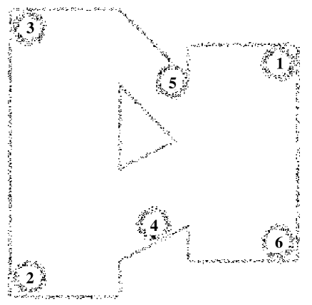
Figure 1: A Multi-Task Environment with six goal zones

We use the six goal areas in order to define six MDPs/tasks. Each of these tasks involves going from one zone to another. The following table sums them up:

MDP	Start	Goal
${\cal M}_{1}$	zone $2$	zone $1$
${\cal M}_{2}$	zone $3$	zone $2$
${\cal M}_{3}$	zone $4$	zone $3$
${\cal M}_{4}$	zone $5$	zone $4$
${\cal M}_{5}$	zone $6$	zone $5$
${\cal M}_{6}$	zone $1$	zone $6$

We have applied the Modular Self-Organization procedure (algorithm 4) with $3$ kernels/modules, and with the $Error()$ and $Learn()$ functions described in section 2. Figure 2 shows that the performances (obtained with $500$ simulated runs for each single task) of the system grow for the six tasks.

Figure 2: Performance evolution during the Modular Self-Organization algorithm: for each of the six MDPs (and for the average cumulative rewards for all six), we see that the system performance is monotonically increasing.

Figure 3: Evolution of the clustering process: at each iteration, each task is naturally associated to one of the six modules (the one that makes the minimal error); this spread over eventually stabilizes: at the end, module $1$ deals with ${\cal M}_{2}$ and ${\cal M}_{3}$, module $2$ deals with ${\cal M}_{4}$ and ${\cal M}_{5}$, and module 3 deals with ${\cal M}_{1}$ and ${\cal M}_{6}$.

Figure 3 shows that the clustering (i.e. the spreading of expertise over the $3$ modules) eventually stabilizes to an interesting clustering: each of the eventual modules deals with two tasks.

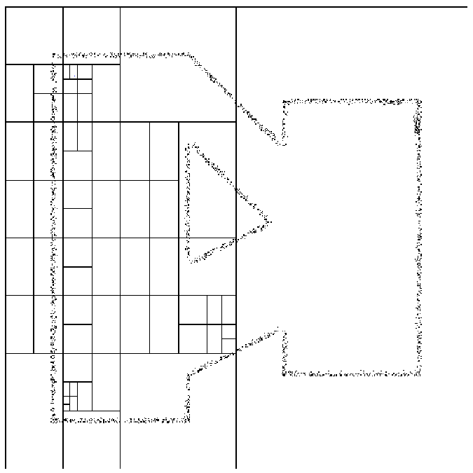
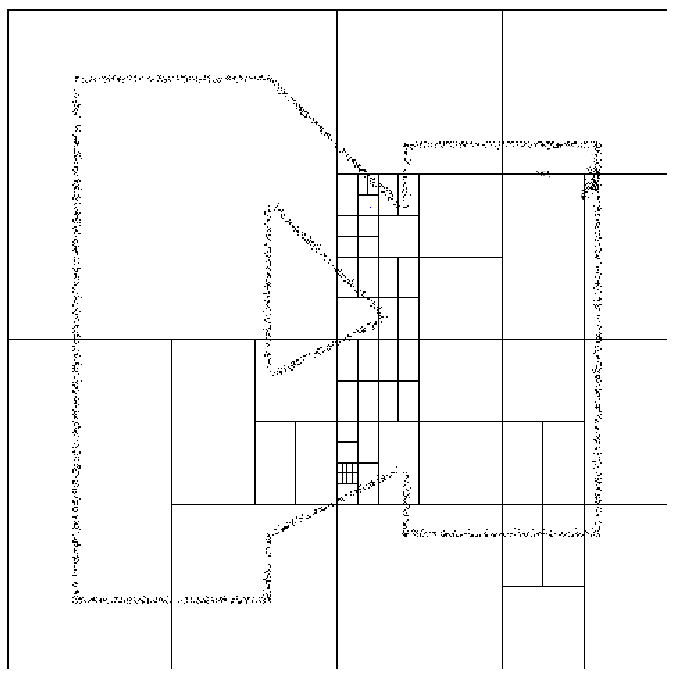
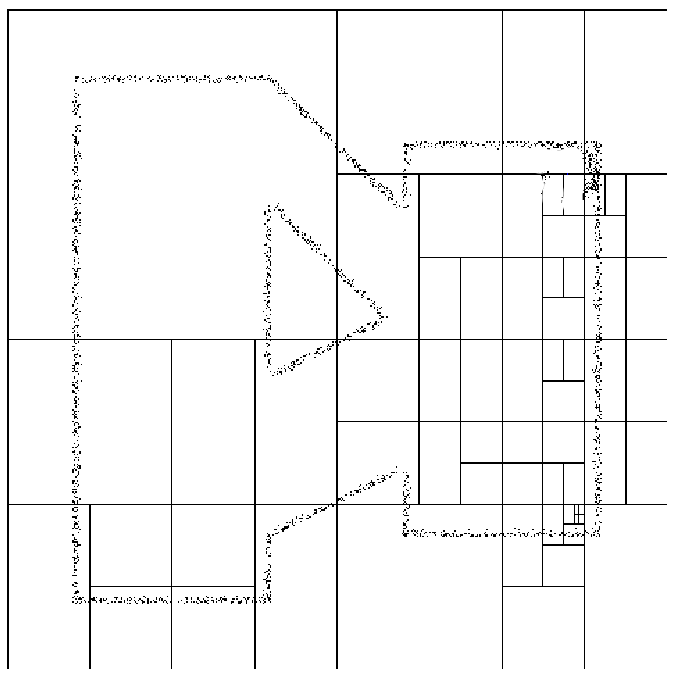
Figure 4: Final State Aggregations of the three modules

Finally, we see in figure 4 the state aggregations of the resulting $3$ modules: we observe that, a module tends to describe precisely the goal zones of its two automatically associated tasks.

6 Conclusion

In this paper, we have reviewed some recent results for sound approximation in large state space Markov Decision Processes and showed how they could be applied to the state aggregation scheme. We have then showed how such results could be extended to an interesting problem: The Modular Self-organizing of an autonomous agent. We have formalized the problem of modular self-organization as a clustering problem in the space of MDPs. We solved it using an on-line version of the Dynamic Cluster algorithm. Finally, we have experimented this approach in a continuous navigation framework, where a $3$-module agent has to address $6$ tasks.

In future works, we will try to extend this general approach to more powerful approximations schemes than the state aggregation approach (which suffers from the curse of dimensionality). Furthermore, we will investigate possible use in reinforcement learning, where the parameters of an MDP have to be obtained by experience.

References

- [1] P. Blanchet. Modular growing network architectures for td learning. In Pattie Maes, Maja J. Mataric, Jean-Arcady Meyer, Jordan B. Pollack, and Stewart W. Wilson, editors, From animals to animats 4, pages 343–352, Cambridge, MA, 1996. MIT Press.
- [2] E. Diday. The dynamic clusters method and optimization in non hierarchical-clustering. In SpringerVerlag, editor, 5th Conference on optimization technique, Lecture Notes in Computer Science 3, pages 241–258, 1973.
- [3] B. Digney. Emergent hierarchical control structures: Learning reactive hierarchical relationships in reinforcement environments, 1996.
- [4] E. Forgy. Cluster analysis of multivariate data: efficiency versus interpretability of classifications. In Biometrics, volume 21, page 768, 1965.
- [5] M. Hauskrecht, N. Meuleau, L. P. Kaelbling, T. Dean, and C. Boutilier. Hierarchical solution of Markov Decision Processes using macro-actions. In Uncertainty in Artificial Intelligence, pages 220–229, 1998.
- [6] R. Jacobs, M. Jordan, and A. Barto. Task decomposition through competition in a modular connectionist architecture: The what and where vision tasks. Cognitive Science, 15:219–250, 1991.
- [7] L. P. Kaelbling. Hierarchical learning in stochastic domains: Preliminary results. In International Conference on Machine Learning, pages 167–173, 1993.
- [8] J. Lange, H. Voigt, and D. Wolf. Growing artificial neural networks based on correlation measures, taske decomposition and local attention neurons, 1994.
- [9] M. L. Littman, T. L. Dean, and L. P. Kaelbling. On the complexity of solving Markov decision problems. In Proceedings of the Eleventh Annual Conference on Uncertainty in Artificial Intelligence (UAI–95), pages 394–402, Montreal, Québec, Canada, 1995.
- [10] R. Munos and A. Moore. Rates of convergence for variable resolution schemes in optimal control. In International Conference on Machine Learning, 2000.
- [11] R. Munos and A. Moore. Variable resolution discretization in optimal control. Machine Learning Journal, 49:291–323, 2002.
- [12] M. Puterman. Markov Decision Processes. Wiley, New York, 1994.
- [13] Richard S. Sutton. On the significance of markov decision processes. In ICANN, pages 273–282, 1997.
- [14] R.S. Sutton and A.G. Barto. Reinforcement Learning, An introduction. BradFord Book. The MIT Press, 1998.
- [15] G. Theocharous, K. Rohanimanesh, and S. Mahadevan. Learning and planning with hierarchical stochastic models for robot navigation. In ICML 2000 Workshop on Machine Learning of Spatial Knowledge, Stanford University, July 2000.