Motion Primitives for Robotic Flight Control

Abstract

We introduce a simple framework for learning aggressive maneuvers in flight control of UAVs. Having inspired from biological environment, dynamic movement primitives are analyzed and extended using nonlinear contraction theory. Accordingly, primitives of an observed movement are stably combined and concatenated. We demonstrate our results experimentally on the Quanser Helicopter, in which we first imitate aggressive maneuvers and then use them as primitives to achieve new maneuvers that can fly over an obstacle.

I Introduction

The role of UAVs (Unmanned Aerial Vehicles) has gained significant importance in the last decades. They have many advantages (agility, low surface area, ability to work in constrained or dangerous places) over their conventional precedents. In addition, current UAVs are more biologically-inspired in terms of shape and performance because of the improvements in electronics and propulsion. Unfortunately, we are still far away from using their capacity at the fullest. This is mostly related with the weakness of current control algorithms against high-dimensional and nonlinear environments. In this sense, generating aggressive maneuvers is interesting and hard to accomplish.

In this paper, our approach to solve this issue is designed in view of the experiments on frogs and monkeys which suggest that we are faced with an inverse-kinematics algorithm that adapts to the environment and changes in a sequence of target points irrespective of the initial conditions. In theory, we analyzed dynamic movement primitives (DMPs)[18] and combined them using contraction theory. In experiments, obstacle avoidance DMP of a human-piloted flight data is segmented into parts and combined at different initial points to achieve maneuvers against different obstacles on different locations. Background of our work is briefly detailed below.

I-A Background

I-A1 Imitation Learning

”By three methods we may learn wisdom: first, by reflection, which is noblest; second, by imitation, which is easiest; and third, by experience, which is the most bitter.” (Confucius) Imitation takes place when an agent learns a behavior by observing the execution of that behavior from a teacher [11]. Imitation is not inherent to humans. It is also observed in animals. For example, experiments show that kittens exposed to adult cats manipulate levers to retrieve food much faster than the control group [28].

There has been a number of applications on imitation learning in the field of robotics. Studies on locomotion [5, 6, 34], humanoid robots [7, 8],[29], [27], and human-robot interactions [33, 20] have used imitation learning or movement primitives. The emphasis on these studies is on primitive derivation and movement classification [30]; combinations of the primitives [21, 16, 22, 23, 44, 42] and primitive models [17, 19, 45, 42] in order to extract behaviors.

I-A2 Aggressive Maneuvers

Aggressive control of autonomous helicopters represents a challenging problem for engineers. The challenge owes itself to the highly nonlinear and unstable nature of the dynamics along with the nonlinear relations for actuator saturation. Nevertheless, we can find successful unmanned helicopter examples [4, 35, 1, 3, 37, 38, 39, 40, 41] in the literature. However, model helicopters controlled by humans can achieve considerably more complex and aggressive maneuvers compared to that can be done autonomously with the state of the art. In [36], it is observed that after several repetitions of the same maneuver, performed by a human, generated trajectories are similar and the control inputs are well-structured and repetitive. Hence, it is intuitive to focus on understanding human’s maneuvers to find proper algorithms for unmanned control.

I-A3 Biological Motivation

In their experiment with deafferented and intact monkeys, Bizzi [24] found that a certain movement can be executed regardless of initial conditions, emphasizing the importance of feedback control. In particular, they have shown that the control variable is the equilibrium state of the agonist and antagonist muscles. Same experimental setup is again used to characterize the trajectory of the motion in [25]. Their results additionally suggest that movement called ”virtual trajectory” is composed of more than one equilibrium point and central nervous system uses the stability of the lower level of the motor system to simplify the generation of movement primitives[25].

Bizzi [31] and Mussa-Ivaldi [26]’s experiments on frogs provide us with further clues in understanding movement primitives. They microstimulated spinal cord and measured the forces at the ankle. Having repeated this process with ankle replaced at nine to 16 locations, they observed that collection of measured forces always converges to a single equilibrium point. In their model, inverse kinematics plays a crucial role in achieving the endpoint trajectory (see Mussa-Ivaldi [32]).

II Analysis of DMP

This section outlines the analysis of the DMP algorithm using contraction theory.

II-A DMP Algorithm

DMP is a trajectory generation algorithm which interpolates between the start and end points of a path based on learning. The system can be represented by

$$\tau\dot{z}=\alpha_{z}(\beta_{z}(g-y)-z)$$ (1)

$$\tau\dot{y}=z+f,$$ (2)

where $y$, $\dot{y}$ and $\ddot{y}$ characterize the desired trajectory, $\alpha_{z}$ and $\beta_{z}$ are time constants, $\tau$ is a temporal scaling factor, $g$ is the desired end point. In addition, the canonical system is given by

$$\tau\dot{v}=\alpha(\beta_{z}(g-x)-v)$$ (3)

$$\tau\dot{x}=v,$$ (4)

In general, assuming that the $f$-function is zero, system will converge to $g$ exponentially. The goal of the DMP algorithm is to modify this exponential path so that the $f$-function makes the system non-linear and allows us to generate desired trajectories between the origin and the $g$ point.

The $f$-function is a normalized linear combination of Gaussians which helps to approximate the final trajectory, i.e. it has the general form

$$f(x,v,g)=\frac{\sum_{i=1}^{N}\Psi_{i}w_{i}v}{\sum_{i=1}^{N}\Psi_{i}},$$ (5)

where

$$\Psi_{i}=exp\{-h_{i}(x/g-c_{i})^{2}\}.$$ (6)

II-B Rhythmic DMPs

The DMP algorithm can also be extended to the rhythmic movements [46] by changing the canonical system with the following:

$$\tau\dot{\phi} = 1$$ (7)

$$\tau\dot{r} = -\mu(r-r_{0})\hskip 42.67912pt\mu>0$$ (8)

where $\phi$ corresponds to $x$ in Eq. 3 as a temporal variable. Similar to the discrete system, control policy:

$$\tau\dot{z} = \alpha_{z}(\beta_{z}(y_{m}-y)-z)$$ (9)

$$\tau\dot{y} = z+f$$ (10)

$$f(x,v,g) = \frac{\sum_{i=1}^{N}\Psi_{i}w_{i}^{T}\tilde{v}}{\sum_{i=1}^{N}\Psi_{i}}$$ (11)

$$\psi = exp\{h_{i}(\cos(\phi-c_{i})-1)\}$$ (12)

where $y_{m}$ is a basis point for learning and $\tilde{v}=[x=r\cos(\phi),y=r\sin(\phi)]^{T}$.

II-C Learning of primitives using DMPs

Learning aspect of the algorithm comes into play with the computation of the weights ($w_{i}$) of the Gaussians. Weights are derived from Eq.1 and Eq.2 using the training trajectory $y_{demo}$ and $\dot{y}_{demo}$ as variables . Once the parameters of the $f$-function are learned, then DMP can simply be used to generate the original trajectory. As detailed below, spatial and temporal shifts are achieved by adjusting the $g$ and $\tau$ respectively.

• Spatial adjustments: The first system [Eq.(1), Eq.(2)] can be seen as a linear system. It is due to the fact that variable $v$ in $f$-function is only multiplied by time-varying constant. Hence, we can say that output ($y$) is simply scaled by $g$ from superposition.

• Temporal adjustments: The second system [(Eq.(3) Eq.(4)] is simply linear. In addition, f function is linear because the multiplier $\Psi_{i}$ is a time-varying constant, temporally scaled by $\tau$. Thus, from linearity, we can say that temporal adjustments of the whole system is carried out by just changing the variable $\tau$.

These arguments can also be extended to the rhythmic DMPs for modulations.

II-D Analysis of DMP Using Contraction Theory

The basic theorem of contraction analysis [14] is stated as

Theorem (Contraction)Consider the deterministic system

$$\dot{x}=f(x,t)$$ (13)

where f is a smooth nonlinear function. If there exist a uniformly invertible matrix associated generalized Jacobian matrix

$$F=(\dot{\Theta}+\Theta\frac{\partial f}{\partial x})\Theta^{-1}$$ (14)

is uniformly negative definite, then all system trajectories converge exponentially to a single trajectory, with convergence rate $|\lambda_{max}|$, where $\lambda_{max}$is the largest eigenvalue of the symmetric part of F. The system is said to be contracting.

Basically, a nonlinear time-varying dynamic system is called contracting if initial conditions or temporary disturbances are forgotten exponentially fast, i.e., if trajectories of the perturbed system return to their nominal behavior with an exponential convergence rate. It turns out that relatively simple conditions can be given for this stability-like property to be verified. Furthermore this property is preserved through basic system combinations, such as parallel combinations, feedback combinations, and series or hierarchies, yielding simple tools for modular design. For linear time-invariant systems, contraction is equivalent to strict stability.

Consider a system

$$\frac{d}{dt}\left[\begin{array}[]{c}\delta z_{1}\\ \delta z_{2}\end{array}\right] = \left[\begin{array}[]{cc}F_{11}&0\\ F_{21}&F_{22}\end{array}\right]\left[\begin{array}[]{c}\delta z_{1}\\ \delta z_{2}\end{array}\right]$$ (21)

where $z_{1}$ and $z_{2}$ represent the first and the second system of DMP and the $\delta z_{i}$ represent associated differential displacements (see [14]) . Equation (21) display a hierarchy of contracting systems, and furthermore since $F_{21}$ is bounded by construction of $f$, the whole system globally exponentially converges to a single trajectory [14].

We can also extend the hierarchical contraction property to the rhythmic DMPs, since the canonical system, which is shown below is contracting.

$$\tau\dot{x}=-\mu(x-x_{0})-y\hskip 28.45274pt\mu>0$$ (22)

$$\tau\dot{y}=-\mu(y-y_{0})+x\hskip 54.06006pt$$ (23)

Although the system will eventually contract to the $g$ point, there will be a time delay due to the hierarchy between second and the first system. We can decrease this delay by increasing the number of weights in our equation.

Using contraction theory, stability of the DMPs can be analyzed. Once the original trajectory is mapped into the DMP, the system behaves linearly for a given input-output relation as shown before. Moreover, contraction property guarantees the convergence into a single trajectory. From linearity, it is easy to show that learning the trajectories is not constrained by the stationary goal points that do not have a velocity components, which are required for equilibrium points in virtual trajectories.

III Coupling of DMPs Using Contraction Theory

In this section, we use partial contraction theory [15] to couple DMPs. One-way coupling configuration of contraction theory allows a system to converge to its coupled pair smoothly. Theory for the one-way coupling states the following two systems:

$$\dot{x}_{1}=f(x_{1},t)$$ (24)

$$\dot{x}_{2}=f(x_{2},t)+u(x_{1})-u(x_{2})$$ (25)

In a given formula, if $f-u$ is contracting, then $x_{2}\rightarrow x_{1}$ from any initial condition.

A typical example for one way coupling is an observer design while the first system represents the real plant and the second system represents the mathematical model of the first system. The states of the second system will converge to the states of the first system and result in the robust estimation of the real system states. However, for our experiments, we interpret contraction as to imitate the transition between two states. It will be shown in section IV how the end of one trajectory becomes the initial condition of the second trajectory and contraction accomplishes the smooth transition.

In DMPs, we couple the two systems using the following equations:

$$\ddot{y}_{1}=g_{1}-y_{1}-\dot{y_{1}}+f(y_{1})$$ (26)

$$\ddot{y}_{2}=g_{2}-y_{2}-\dot{y_{2}}+u(y_{1})-u(y_{2})$$ (27)

$$u(x_{i})=g_{i}+f(x_{i})$$ (28)

$$f(x,v,g)=\frac{\sum_{i=1}^{N}\Psi_{i}w_{i}v}{\sum_{i=1}^{N}\Psi_{i}}$$ (29)

$$\Psi_{i}=exp\{-h_{i}(x/g-c_{i})^{2}\}$$ (30)

A toy example of the equations listed above can be seen in Fig. 1. In this setting, $y_{2}$ is the first trajectory primitive, which contracts to $y_{1}$ – the second trajectory primitive.

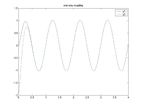
Figure 1: One-way coupling of a rhythmic DMPs

One-way coupling has many advantages as a method over its precedents:

In [42], trajectories are achieved by simply stretching the original trajectory in its coordinates and there is a direct relation between initial and end points. Also, there are discontinuities in terms of derivatives of the trajectory at the transition regions between primitives. Giese [43] solves the problem of discontinuities by first taking the derivatives of the original trajectories, then combining the derivatives, and finally integrating them again using initial conditions. However, this method adversely affects the accuracy of the trajectories. Hence, our method improves on [42] and [43] by generating more accurate trajectories independent of initial points.

In [2], snapshots of the pilot’s maneuvers are taken and evaluated as noisy measurements of hidden and true trajectory. In their model, time indexes are used for the comparison of expert’s demonstrations. Maximization of the joint likelihood of demonstrations are achieved through trajectory learning algorithms. As was done in [1], Locally Weighted Learning is used for learning system dynamics close to trajectories. Moreover, desired trajectories are supervised by adding information specific to each maneuver. With the help of feasible trajectory, optimal controller and system dynamics along the maneuver, they achieved remarkable results on model helicopters. However, finding hidden trajectory requires noteworthy computational performance where they smooth out data to emphasize the similarities. In addition, their algorithm applies only for mimicking demonstrations. In our algorithm, learning the hidden and true trajectory of maneuvers can simply be done by comparing the weights of DMPs (see [18]). It is also easier to manipulate DMPs by changing parameters ($\tau$ and $g$) for new challenges. Moreover, our method lies on the background of biological experiments in such a way that it is adaptable for further research.

In general, we summarize the advantages for using dynamical systems as control policies as follows:

• It is easy to incorporate perturbations to dynamical systems.

• It is easy to represent the primitives.

• Convergence to the goal position is guaranteed due to the attractor dynamics of DMP.

• It is easy to modify for different tasks.

• At the transition regions, discontinuities are avoided.

• Partial contraction theory forces the coupling from any initial condition.

Also in [18], Schaal’s suggested system is driven between stationary points. However, biological experiments suggest that we are faced with a ”virtual trajectory” composed of equilibrium points that has velocity components. For this reason, we showed that we can achieve this property by combining nonconstant points.

IV Experiments on Helicopter

Here, we apply the motion primitives on the helicopter.

IV-A Experimental Setup

We used Quanser Helicopter (see Figure 2) in our experiments. The helicopter is an under-actuated system having two propellers at the end of the arm. Two DC motors are mounted below the propellers to create the forces which drive propellers. The motors’ axes are parallel and their thrust is vertical to the propellers. We have three degrees of freedom (DOF): pitch (vertical movement of the propellers), roll (circular movement around the axis of the propellers) and travel (movement around the vertical base) in contrast with conventional helicopters with six degrees of freedom.

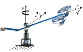
Figure 2: Transverse momentum distributions.[9]

In system model[9], the origin of our coordinate system is at the bearing and slip-ring assembly. The combinations of actuators form the collective $(T_{col}=T_{L}+T_{R})$ and cyclic $(T_{cyc}=T_{L}-T_{R})$ forces which are used as inputs in our controller. The schematics of helicopter are shown in Figures  4 and 4.

Figure 3: Schematic of the 3DOF helicopter.[9]

Figure 4: Top view. [9]

Let $J_{xx}$, $J_{yy}$, and $J_{zz}$ denote the moment of inertia of our system dynamics. For simplicity, we ignore the products of inertia terms. The equations of motion are as follows (cf. Ishutkina [9]):

$$J_{zz}\ddot{\psi}=(T_{L}+T_{R})L\cos(\theta)\sin(\phi),$$

$$-(T_{L}-T_{R})l_{h}\sin(\theta)\sin(\phi)-\mbox{Drag},$$

$$J_{yy}\ddot{\theta}=-Mgl_{\theta}\sin(\theta+\theta_{0})+(T_{L}+T_{R})L\cos(\phi),$$

$$J_{xx}\ddot{\phi}=-mgl_{\phi}\sin(\phi)+(T_{L}-T_{R})l_{h},$$

where

• $M$ is the total mass of the helicopter assembly,

• $m$ is the mass of the rotor assembly,

• $L$ is the length of the main beam from the slip-ring pivot to the rotor assembly,

• $\psi$, $\theta$, $\phi$ are travel, pitch and roll angles respectively.

• $l_{h}$ is the distance from the rotor pivot to each of the propellers,

• $\mbox{Drag}=\frac{1}{2}\rho(\dot{\psi}L)^{2}(S_{0}+S_{0}^{\prime}\sin(\phi))L$,

• $S_{0}$ and $S_{0}^{\prime}$ are the effective drag coefficients times the reference area and $\rho$ is the density of air.

It can be seen that the above system is nonlinear in the states, but linear in terms of control inputs. In practice, we used feedback linearization with bounded internal dynamics (see Bayraktar [12]) for a 3DOF helicopter, which tracks trajectories in elevation and travel.

IV-B Simulation & Experimental Results

In this section, we first describe our numerical simulation of the proposed primitive framework. Second, we describe our actual experiment on the Quanser Helicopter.

IV-B1 Trajectory Generation

In experimental setup, we used an operator with a joystick to create aggressive trajectories to pass an obstacle. However, generating aggressive trajectories with the joystick is a difficult task even for the operator. Therefore, we designed an augmented control for the joystick to enhance the performance of the helicopter. In detail, we used ”up” and ”down” movements of the joystick to increase or decrease the $T_{col}$ that is applied to the actuators. For the ”right” and ”left” movements of the joystick, we preferred to control the roll angle using PD control.

In the original maneuver, the obstacle’s distance and the highest point are in the coordinates where $\psi$ and $\theta$ angles are $220$ and $60$ respectively and the helicopter stops at the coordinates where $\psi=28$, $\theta=317$ and $\phi=-17$ (see Figure 5).

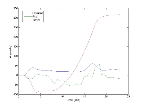
Figure 5: Original maneuver achieved by an operator

IV-B2 Trajectory Learning

From several demonstrations, it is observed that our operator follows two distinct pattern to carry out the maneuver. Accordingly, these two patterns suggest an equilibrium point at the top of the obstacle. Therefore, to fly over different obstacles, the acquired primitive is segmented into two primitives at the highest pitch angle. Fig. 6 and Fig. 7 show the results of DMP algorithm for the pitch angle. The top left graphs are results for pitch angles, where green lines represent the operator input for the trajectories and blue lines represent the fittings that the DMP computes for different start and end points. Hence, desired trajectories in these graphs are not on top of the trajectories generated by the operator. Other graphs show the time evolution of the DMP parameters.

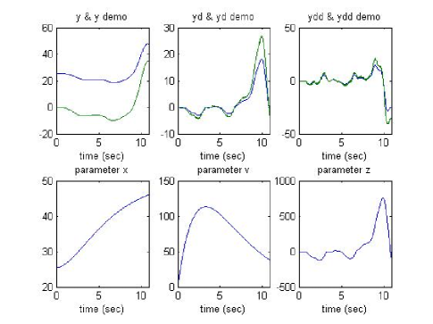
Figure 6: Trajectory generation for the first primitive - pitch

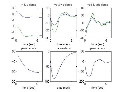
Figure 7: Trajectory generation for the second primitive - pitch

IV-B3 Synchronization of primitives

The two primitives created in the previous sections are defined as trajectories between certain start and end points. However, the end point of the first trajectory does not necessarily matches with the starting point of the second trajectory. We use partial contraction theory [15] to force the first trajectory to converge to the second one. However, since we want to use the contraction as a transition between two trajectories, coupling is enabled towards the end of first primitive. Figure 8 shows how the two trajectories evolve in time. In the first primitive, the goal positions of $\psi$ and $\theta$ angles are changed to $150^{\circ}$ and $50^{\circ}$ respectively, where original angles are $\psi=220^{\circ}$ and $\theta=60^{\circ}$. In the second primitive, the goal position of the $\psi$ angle is changed from $317^{\circ}$ to $300^{\circ}$.

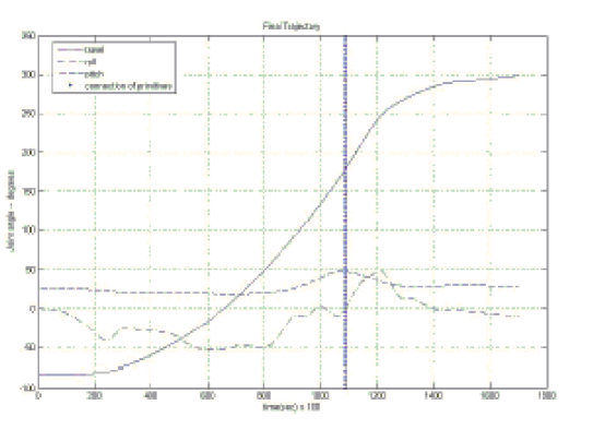
Figure 8: Time evolution of primitive-1 and primitive-2 merged.

IV-B4 Experiments on the Helicopter

Tracking performance of the helicopter is shown in Figure 9. It is seen that the helicopter followed the desired ($\psi$ and $\theta$) angles almost perfectly. However, the trajectory of the roll angle is a bit different than the desired since we control two parameters ($\psi$ and $\theta$) and the goal positions of the DMPs are different. But we should highlight the fact that two roll trajectories follow the same pattern. In figure, the last part of the roll trajectory manifests an oscillation which can be prevented by roll control, since the other parameters are almost constant. The tracking performance can further be improved by applying discrete nonlinear observers to get better velocity and acceleration values. Figure 10 shows snapshots of the maneuver.

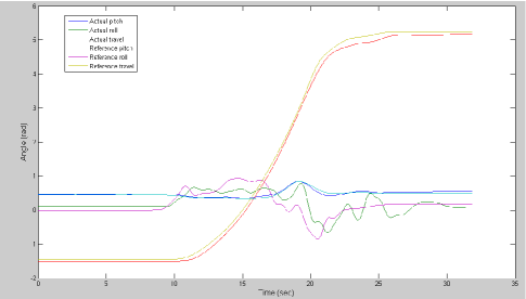
Figure 9: Tracking performance of the helicopter.

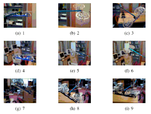
Figure 10: Snapshots of the obstacle avoidance maneuver.

V Extensions of DMP

V-A Dynamical System with First-Order Filters

DMP algorithm can be improved by replacing the first system with the equations shown below:

$$\tau\dot{y}+a_{1}y=x$$ (31)

$$\tau\dot{x}+a_{2}x=g+f$$ (32)

which is equivalent of

$$\tau^{2}\ \ddot{y}+\tau\ (a_{1}+a_{2})\ \dot{y}+a_{1}a_{2}\ y\ =\ g+f$$ (33)

By introducing two first-order filters, we guarantee the stability of the system against time varying parameters like $\tau(t)$ or $g(t)$ . Since the system is linear without the $f$-function (Eq.11), we achieve learning and modulation properties of DMP using the $f$ in either Eq.(31) or Eq.(32). For further applications, we will use this model to generate primitives for time-varying goal points.

V-B Generating New Primitives

Experiments on frog’s spinal cord [31, 26, 47] suggest that movement primitives can be generated from linear combinations of vectorial force fields which lead the limb of a frog to the virtual equilibrium points. In [47], it is also pointed out that vectorial summation of two force fields with different equilibrium points generate a new force field whose equilibrium point is at intermediate location of the original equilibrium points. In this perspective, we will use two methods to generate new primitives.

V-B1 Two-way Synchronization of DMPs

Consider a system

$$\ddot{y}_{1}=f(y_{1},t)+K(u(y_{2})-u(y_{1}))\;\;\;\;\;\;\;\;\;\;\;\;$$ (34)

$$\ddot{y}_{2}=f(y_{2},t)+K(u(y_{1})-u(y_{2}))\;\;K>0$$ (35)

Where $y_{1}$ and $y_{2}$ represent the first and the second primitive respectively. From partial contraction theory, we say that $y_{1}$ and $y_{2}$ converge together exponentially, if $f-2Ku$ is contracting. Since DMPs are already contracting, we achieve synchronization using contracting inputs. In Fig.11 (top), new primitive is a linear combination of sine and cosine primitives. Also in the same figure, coupling forces accounts for oscillations before synchronization happens.

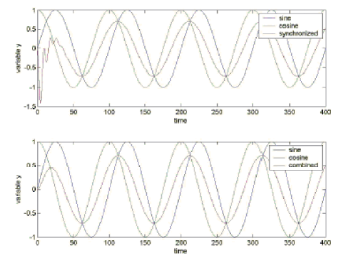
Figure 11: Top:Synchronization of sine and cosine primitives. Bottom: New primitive generated by the linear combinations of weights from sine and cosine primitives

V-B2 Combination of Primitives using Weights

In DMPs, as it was shown before, system behaves linearly and superposition applies. Therefore, in the $f$-function , linear combination of the weights from different primitives produce linear combination of primitives. For rhythmic DMPs, as an example, we combine the weights of the sine and cosine primitives ($w_{new}=0.5w_{sine}+0.5w_{cosine}$) to generate a new primitive (See Fig. 11 (bottom)). However for a regular DMP, we can not achieve the desired trajectories although we have linearity which is because input ”$g$” point is not compatible with the weights changing with respect to the couplings. For this reason, we will simply modify the equations in our later research.

VI Conclusion

In this paper, we use a novel approach, inspired by biological experiments and humanoid robotics, which uses control primitives to imitate the data taken from human-performed obstacle avoidance maneuver. In our model, DMP computes the trajectory dynamics so that we can generate complex primitive trajectories for given different start and end points, while one-way coupling ensures smooth transitions between primitives at the equilibrium points. We demonstrate our algorithm with an experiment. We generate a complex, aggressive maneuver, which our helicopter could follow within a given error bound with a desired speed. Future research will be conducted on different combinations of primitives using partial contraction theory. We expect these techniques to be particularly useful when the system dynamic models are very coarse, as e.g. in the case of flapping wing systems and new bio-inspired underwater vehicles.

References

- [1] A.Y. Ng, Daishi Harada and Shankar Sastry. Autonomous Helicopter Flight via Reinforcement Learning. In Neural Information Processing Systems 16, 2004
- [2] A. Coates, P. Abbeel, A.Y. Ng. Learning for Control from Multiple Demonstrations. In Proceedings of the Twenty-fifth International Conference on Machine Learning, 2008.
- [3] J. Bagnell and J. Schneider. Autonomous Helicopter Control using Reinforcement Learning Policy Search Methods. In International Conf. Robotics and Automation. IEEE, 2001.
- [4] T. Schouwenaars, B. Mettler, E. Feron, and J. How. Hybrid architecture for full-envelope autonomous rotorcraft guidance. In American Helicopter Society 59th Annual Forum, 2003.
- [5] G. Taga, Y. Yamaguchi, H. Shimizu. Self-organized Control of Bipedal Locomotion by Neural Oscillators in Unpredictable Environment. In Biological Cybernetics, 1991.
- [6] G. Taga. A Model of Neuro-musculo-skelatal System for Human Locomotion. In Biological Cybernetics, 1995.
- [7] S. Schaal, D. Sternad, and C. Atkeson, One Handed Juggling : A Dynamical Approach to a Rhytmic Movement Task. In Journal of Motor Behaviour, 1996.
- [8] J. A. Ijspert, J. Nakanishi, and S. Schaal. Learning Rhythmic Movements by Demonstration Using Nonlinear Oscillators. In International Conf. Robotics and Automation. IEEE, 2000.
- [9] M. Ishutkina. Design and implimentation of a supervisory safety controller for a 3DOF helicopter. Master’s thesis, Massachusetts Institute of Technology, 2004.
- [10] S. Bayraktar. Aggressive Landing Maneuvers for Unmanned Aerial Vehicles. Master’s thesis, Massachusetts Institute of Technology, 2004.
- [11] P. Bakker and Y. Kuniyoshi. Robot See, Robot Do: An Overview of Robot Imitation. AISB’96 Workshop on Learning in Robots and Animals, 1996.
- [12] S. Bayraktar, M. Ishutkina. Nonlinear Control of a 3 DOF Helicopter. 2.152, Nonlinear Control System Design, Project Report, 2004.
- [13] J.J. Slotine and W. Li. Applied Nonlinear Control, Prentice-Hall, 1991.
- [14] W. Lohmiller, J.J. Slotine. On Contraction Analysis for Nonlinear Systems. Automatica 34(6), 1998.
- [15] W. Wang, J.J. Slotine. On Partial Contraction Analysis for Coupled Nonlinear Oscillators.Biological Cybernetics, 2004.
- [16] W. Lohmiller, J.J.E. Slotine. Applications of Contraction Analysis. Proc. of the 36th CDC San Diego, CA, 1997.
- [17] S. Schaal, J. Peters, J. Nakanishi, A. Ijspeert. Control, planning, learning, and imitation with dynamic movement primitives. IEEE/RSJ International Conference on Intelligent Robots and Systems, 2003.
- [18] A.J. Ijspeert, J. Nakanishi, S. Schaal. Movement imitation with nonlinear dynamical systems in humanoid robots. ICRA, 2002.
- [19] F.A. Mussa-Ivaldi, S.A. Solla. Neural primitives for motion control. IEEE Journal of Oceanic Engineering, 2004.
- [20] M.N. Nicolescu, M. Mataric. Task learning through imitation and human-robot interaction. Proceedings of the second international joint conference on Autonomous agents and multiagent systems, 2003.
- [21] S. Nakaoka, A. Nakazawa, K. Yokoi, K. Ikeuchi. Generating whole body motions for a biped humanoid robot from captured human dances. ICRA, 2003.
- [22] R.R. Burridge, A.A. Rizzi, D.E. Koditschek. Sequential composition of dynamically dexterous robot behaviors. International Journal of Robotics Research, 1999.
- [23] T. Inamura, I. Toshima, Y. Nakamura. Acquisition and embodiment of motion elements in closed mimesis loop. ICRA,2002.
- [24] A. Polit, E. Bizzi. Characteristic of Motor Programs Underlying Arm Movements in Monkeys.Journal of Neurophsiology, 1979.
- [25] E. Bizzi, F.A. Mussa-Ivaldi, N. Hogan. Regulation of multi-joint arm posture and movement. Progress in Brain Research, Vol. 64, 1986.
- [26] F.A. Mussa-Ivaldi, S. Giszter, E. Bizzi. Motor Space Coding in the Central Nervous System. Cold Spring Harb Symp Quant Biol Vol. 55 ., 1990.
- [27] L. Berthouze, P. Bakker and Y. Kuniyoshi. Learning of Oculo-Motor Control: a Prelude to Robotic Imitation. Proc. IROS, 1996.
- [28] B.G. Galef. Imitation in animals: History, definition and interpretation of data from the psychological laboratory. Social Learning: Psychological and Biological Perspectives, 1988.
- [29] A. Billard, M. J. Mataric. Learning human arm movements by imitation: evaluation of a biologically inspired connectionist architecture. Robotics and Autonomous Systems
- [30] A. Fod, M.J Mataric, O.D. Jenkins. Automated Derivation of Primitives for Movement Classification. Autonomous Robots, 2002.
- [31] E. Bizzi, F.A. Mussa-Ivaldi, S. Giszter. Computations underlying the execution of movement: a biological perpective. Science 253, 1991.
- [32] F.A. Mussa-Ivaldi, E. Bizzi. Motor learning Through the Combination of Primitives. Philosophical Transactions of the Royal Society B: Biological Sciences, 2000.
- [33] F.A. Mussa-Ivaldi, J.L. Platton. Robots can teach people how to move their arm. ICRA, 2000.
- [34] A. Billard, A.J. Ijspeert. Biologically inpired neural controllers for motor control in a quadruped robot. IEEE-INNS-ENNS International Joint Conference on Neural Networks, Volume 6, 2000.
- [35] E. Frazzoli, M.A. Dahleh, E. Feron. Maneuver-based motion planning for nonlinear systems with symmetries. IEEE Trans. on Robotics, 2005.
- [36] V. Gavrilets, E. Frazzoli, B. Mettler, M. Piedmonte, E. Feron. Aggressive maneuvering of small autonomous helicopters: a human centered approach. Internatiaonal Journal of Robotics Research, 2001.
- [37] V. Gavrilets, I. Martinos, B. Mettler, E. Feron . Control logic for automated aerobatic flight of a miniature helicopter. AIAA Guidance, Navigation, and Control Conference and Exhibit, Monterey, California, 2002.
- [38] R. Mahony, R. Lozano. (Almost) Exact path tracking control for an autonomous helicopter in hover manoeuvres. ICRA, 2000.
- [39] O. Shakernia, Y. Ma, T. J. Koo, S. Sastry. Asian Journal of Control, 1(3):128–145, 1999.
- [40] D.H. Shim, H.J. Kim, S. Sastry. Control system design for rotorcraft-based unmanned aerial vehicles using time-domain system identification. Proceedings of the 2000 IEEE International Conference on Control Applications, 2000.
- [41] B. Mettler, E. Bachelder. Combining on- and offline optimization techniques for efficient autonomous vehicle’s trajectory planning. AIAA Guidance, Navigation, and Control Conference and Exhibit, 2005.
- [42] W. Ilg, G.H. Bakir, J. Mezger, M.A. Giese. On the representation, learning and transfer fo spatio-temporal movement characteristics. International Journal of Humanoid Robotics, 2004.
- [43] J. Mezger, W. Ilg, M.A. Giese. Trajectory synthesis by hierarchial spatio-temporal correspondence: comparison of different methods. Proceedings of the 2nd symposium on Applied perception in graphics and visualization, 2005.
- [44] L. Sentis, O. Khatib. Synthesis of whole-body behaviors through hierarchial control of behavioral primitives. International Journal of Humanoid Robotics, 2005.
- [45] F. A. Mussa-Ivaldi. Nonlinear force fields: a distributed system of control primitives for representing an learning movements. IEEE International Symposium on Computational Intelligence in Robotics and Automation, 1997.
- [46] A. Ijspeert, J. Nakanishi, and S. Schaal. Learning attractor landscapes for learn- ing motor primitives. In in Advances in Neural Information Processing Systems 15, 2003.
- [47] F.A. Mussa-Ivaldi, S.F. Giszter, and E. Bizzi. Linear combinations of primitives in vertebrate motor control. In Proceedings of the National Academy of Sciences, 1994.