MDL Denoising Revisited

Abstract

We refine and extend an earlier MDL denoising criterion for wavelet-based denoising. We start by showing that the denoising problem can be reformulated as a clustering problem, where the goal is to obtain separate clusters for informative and non-informative wavelet coefficients, respectively. This suggests two refinements, adding a code-length for the model index, and extending the model in order to account for subband-dependent coefficient distributions. A third refinement is derivation of soft thresholding inspired by predictive universal coding with weighted mixtures. We propose a practical method incorporating all three refinements, which is shown to achieve good performance and robustness in denoising both artificial and natural signals.

I Introduction

Wavelets are widely applied in many areas of signal processing [1], where their popularity owes largely to efficient algorithms on the one hand and advantages of sparse wavelet representations on the other. The sparseness property means that while the distribution of the original signal values may be very diffuse, the distribution of the corresponding wavelet coefficients is often highly concentrated, having a small number of very large values and a large majority of very small values [2]. It is easy to appreciate the importance of sparseness in signal compression,  [3, 4]. The task of removing noise from signals, or denoising, has an intimate link to data compression, and many denoising methods are explicitly designed to take advantage of sparseness and compressibility in the wavelet domain, see e.g., [5]–[7].

Among the various wavelet-based denoising methods those suggested by Donoho and Johnstone [8, 9] are the best known. They follow the frequentist minimax approach, where the objective is to asymptotically minimize the worst-case $L^{2}$ risk simultaneously for signals, for instance, in the entire scale of Hölder, Sobolev, or Besov classes, characterized by certain smoothness conditions. By contrast, Bayesian denoising methods minimize the expected (Bayes) risk, where the expectation is taken over a given prior distribution supposed to govern the unknown true signal  [10, 11]. Appropriate prior models with very good performance in typical benchmark tests, especially for images, include the class of generalized Gaussian densities  [6, 12, 13], and scale-mixtures of Gaussians [14, 15] (both of which include the Gaussian and double exponential densities as special cases).

A third approach to denoising is based on the minimum description length (MDL) principle [16]–[19]. Several different MDL denoising methods have been suggested [6, 12, 20]–[24]. We focus on what we consider as the most pure MDL approach, namely that of Rissanen [23]. Our motivation is two-fold: First, as an immediate result of refining and extending the earlier MDL denoising method, we obtain a new practical method with greatly improved performance and robustness. Secondly, the denoising problem turns out to illustrate theoretical issues related to the MDL principle, involving the problem of unbounded parametric complexity and the necessity of encoding the model class. The study of denoising gives new insight to these issues.

Formally, the denoising problem is the following. Let $y^{n}=(y_{1},\ldots,y_{n})^{T}$ be a signal represented by a real-valued column vector of length $n$. The signal can be, for instance, a time-series or an image with its pixels read in a row-by-row order. Let ${\mathcal{W}}$ be an $n\times m$ regressor matrix whose columns are basis vectors. We model the signal $y^{n}$ as a linear combination of the basis vectors, weighted by coefficient vector $\beta^{n}=(\beta_{1},\ldots,\beta_{m})^{T}$, plus Gaussian i.i.d. noise:

$$y^{n}={\mathcal{W}}\beta^{m}+\epsilon^{n},\quad\epsilon_{i}{\overset{\mathit{i.i.d.}}{\sim}}{\mathcal{N}}(0,\sigma_{N}^{2}),$$ (1)

where $\sigma_{N}^{2}$ is the noise variance. Given an observed signal $y^{n}$, the ideal is to obtain a coefficient vector $\tilde{\beta}^{m}$ such that the signal given by the transform $\tilde{y}^{n}={\mathcal{W}}\tilde{\beta}^{m}$ contains the informative part of the observed signal, and the difference $y^{n}-\tilde{y}^{n}$ is noise.

For technical convenience, we adopt the common restriction on ${\mathcal{W}}$ that the basis vectors span a complete orthonormal basis. This implies that the number of basis vectors is equal to the length of the signal, $m=n$, and that all the basis vectors are orthogonal unit vectors. There are a number of wavelet transforms that conform to this restriction, for instance, the Haar transform and the family of Daubechies transforms [1, 25]. Formally, the matrix ${\mathcal{W}}$ is of size $n\times n$ and orthogonal with its inverse equal to its transpose. Also the mapping $\beta^{n}\mapsto{\mathcal{W}}\beta^{n}$ preserves the Euclidean norm, and we have Parseval’s equality:

$$||\beta^{n}||=\sqrt{\langle\beta^{n},\beta^{n}\rangle}=\sqrt{\langle{\mathcal{W}}\beta^{n},{\mathcal{W}}\beta^{n}\rangle}=||{\mathcal{W}}\beta^{n}||.$$ (2)

Geometrically this means that the mapping $\beta^{n}\mapsto{\mathcal{W}}\beta^{n}$ is a rotation and/or a reflection. From a statistical point of view, this implies that any spherically symmetric density, such as Gaussian, is invariant under this mapping. All these properties are shared by the mapping $y^{n}\mapsto{\mathcal{W}}^{T}y^{n}$. We call $\beta^{n}\mapsto{\mathcal{W}}\beta^{n}$ the inverse wavelet transform, and $y^{n}\mapsto{\mathcal{W}}^{T}y^{n}$ the forward wavelet transform. Note that in practice the transforms are not implemented as matrix multiplications but by a fast wavelet transform similar to the fast Fourier transform (see [1]), and in fact not even the matrices need be written down.

For complete bases, the conventional maximum likelihood (least squares) method obviously fails to provide denoising unless the coefficients are somehow restricted since the solution $\tilde{\beta}^{n}={\mathcal{W}}^{T}y^{n}$ gives the reconstruction $\tilde{y}^{n}={\mathcal{W}}{\mathcal{W}}^{T}y^{n}=y^{n}$ equal to the original signal, including noise. The solution proposed by Rissanen [23] is to consider each subset of the basis vectors separately and to choose the subset that allows the shortest description of the data at hand. The length of the description is determined by the normalized maximum likelihood (NML) code length.

The NML model involves an integral, which is undefined unless the range of integration (the support) is restricted. This, in turn, implies hyper parameters, which have received increasing attention in various contexts involving, e.g., Gaussian, Poisson and geometric models [17, 19, 26]–[29]. Rissanen used renormalization to remove them and to obtain a second-level NML model. Although the range of integration has to be restricted also in the second-level NML model, the range for ordinary regression problems does not affect the resulting criterion and can be ignored. Roos et al. [30] give an interpretation of the method which avoids the renormalization procedure and at the same time gives a simplified view of the denoising process in terms of two Gaussian distributions fitted to informative and non-informative coefficients, respectively. In this paper we carry this interpretation further and show that viewing the denoising problem as a clustering problem suggests several refinements and extensions to the original method.

The rest of this paper is organized as follows. In Sec. II we reformulate the denoising problem as a task of clustering the wavelet coefficients in two or more sets with different distributions. In Sec. III we propose three different modifications of Rissanen’s method, suggested by the clustering interpretation. In Sec. IV the modifications are shown to significantly improve the performance of the method in denoising both artificial and natural signals. The conclusions are summarized in Sec. V.

II Denoising and Clustering

II-A Extended Model

We rederive the basic model (1) in such a way that there is no need for renormalization. This is achieved by inclusion of the coefficient vector $\beta$ in the model as a variable and by selection of a (prior) density for $\beta$. While the resulting NML model will be equivalent to Rissanen’s renormalized solution, the new formulation is easier to interpret and directly suggests several refinements and extensions.

Consider a fixed subset $\gamma\subseteq\{1,\ldots,n\}$ of the coefficient indices. We model the coefficients $\beta_{i}$ for $i\in\gamma$ as independent outcomes from a Gaussian distribution with variance $\tau^{2}$. In the basic hard threshold version all $\beta_{i}$ for $i\notin\gamma$ are forced to equal zero. Thus the extended model is given by

$$y^{n}={\mathcal{W}}\beta^{n}+\epsilon^{n},\quad\begin{cases}\epsilon_{i}{\overset{\mathit{i.i.d.}}{\sim}}{\mathcal{N}}(0,\sigma_{N}^{2}),\\ \beta_{i}{\overset{\mathit{i.i.d.}}{\sim}}{\mathcal{N}}(0,\tau^{2}),&\mbox{if $i\in\gamma$,}\\ \beta_{i}=0,&\mbox{otherwise.}\end{cases}$$ (3)

This way of modeling the coefficients is akin to the so called spike and slab model often used in Bayesian variable selection [31, 32] and applications to wavelet-based denoising [33, 34] (and references therein). In relation to the sparseness property mentioned in the introduction, the ‘spike’ consists of coefficients with $i\notin\gamma$ that are equal to zero, while the ‘slab’ consists of coefficients with $i\in\gamma$ described by a Gaussian density with mean zero. This is a simple form of a scale-mixture of Gaussians with two components. In Sec. III-B we will consider a model with more than two components.

Let ${c}^{n}=\beta^{n}+{\mathcal{W}}^{T}\epsilon^{n}$, where ${\mathcal{W}}^{T}\epsilon^{n}$ gives the representation of the noise in the wavelet domain. The vector ${c}^{n}$ is the wavelet representation of the signal $y^{n}$, and we have

$$y^{n}={\mathcal{W}}\beta^{n}+{\mathcal{W}}{\mathcal{W}}^{T}\epsilon^{n}={\mathcal{W}}{c}^{n}.$$

It is easy to see that the maximum likelihood parameters are obtained directly from

$$\hat{\beta}_{i}=\begin{cases}{c}_{i},&\mbox{if $i\in\gamma$,}\\ 0,&\mbox{otherwise.}\end{cases}$$ (4)

The i.i.d. Gaussian distribution for $\epsilon^{n}$ in (3) implies that the distribution of ${\mathcal{W}}^{T}\epsilon^{n}$ is also i.i.d. and Gaussian with the same variance, $\sigma_{N}^{2}$. As a sum of two independent random variates, each ${c}_{i}$ has a distribution given by the convolution of the densities of the summands, $\beta_{i}$ and the $i$th component of ${\mathcal{W}}^{T}\epsilon^{n}$. In the case $i\notin\gamma$ this is simply ${\mathcal{N}}(0,\sigma_{N}^{2})$. In the case $i\in\gamma$ the density of the sum is also Gaussian, with variance given by the sum of the variances, $\tau^{2}+\sigma_{N}^{2}$. All told, we have the following simplified representation of the extended model where the parameters $\beta^{n}$ are implicit:

$$y^{n}={\mathcal{W}}{c}^{n},\quad{c}_{i}{\overset{\mathit{i.i.d.}}{\sim}}\begin{cases}{\mathcal{N}}(0,\sigma_{I}^{2}),&\mbox{if $i\in\gamma$,}\\ {\mathcal{N}}(0,\sigma_{N}^{2}),&\mbox{otherwise,}\end{cases}$$ (5)

where $\sigma_{I}^{2}{\;:=\;}\tau^{2}+\sigma_{N}^{2}$ denotes the variance of the informative coefficients, and we have the important restriction $\sigma_{I}^{2}\geq\sigma_{N}^{2}$ which we will discuss more below.

II-B Denoising Criterion

The task of choosing a subset $\gamma$ can now be seen as a clustering problem: each wavelet coefficient belongs either to the set of the informative coefficients with variance $\sigma_{I}^{2}$, or the set of non-informative coefficients with variance $\sigma_{N}^{2}$. The MDL principle gives a natural clustering criterion by minimization of the code-length achieved for the observed signal (see [35]). Once the optimal subset is identified, the denoised signal is obtained by setting the wavelet coefficients to their maximum likelihood values (4); i.e., retaining the coefficients in $\gamma$ and discarding the rest, and doing the inverse transformation. It is well known that this amounts to an orthogonal projection of the signal to the subspace spanned by the wavelet basis vectors in $\gamma$.

The code length under the model (5) depends on the values of the two parameters, $\sigma_{I}^{2}$ and $\sigma_{N}^{2}$. The standard solution in such a case is to construct a single representative model for the whole model class such that the representative model is universal (can mimic any of the densities in the represented model class). The minimax optimal universal model (see [36]) is given by the so called normalized maximum likelihood (NML) model, originally proposed by Shtarkov [37] for data compression. We now consider the NML model corresponding to the extended model (5) with the index set $\gamma$ fixed.

Denote by $k=k(\gamma)$ the number of coefficients for which $i\in\gamma$. The NML density under the extended model (5) for a given coefficient subset $\gamma$ is defined as

$$f_{\text{\emph{nml}}}(y^{n}\;;\;\gamma):=\frac{f(y^{n}\;;\;\hat{\sigma}^{2}_{I},\hat{\sigma}^{2}_{N})}{C_{\gamma}},$$

where $\hat{\sigma}^{2}_{I}=\hat{\sigma}^{2}_{I}(y^{n})$ and $\hat{\sigma}^{2}_{N}=\hat{\sigma}^{2}_{N}(y^{n})$ are the maximum likelihood parameters for the data $y^{n}$, and $C_{\gamma}$ is the important normalizing constant. The constant $C_{\gamma}$ is also known as the parametric complexity of the model class defined by $\gamma$.

Restricting the data such that the maximum likelihood parameters satisfy

$$\sigma^{2}_{\min}\leq\hat{\sigma}_{N}^{2},\hat{\sigma}_{I}^{2}\leq\sigma^{2}_{\max},$$

and ignoring the constraint $\sigma_{N}^{2}\leq\sigma_{I}^{2}$, the code length under the extended model (5) is approximated by

$$\frac{n-k}{2}\ln\frac{S(y^{n})-S_{\gamma}(y^{n})}{n-k}+\frac{k}{2}\ln\frac{S_{\gamma}(y^{n})}{k}+\frac{1}{2}\ln k(n-k),$$ (6)

plus a constant independent of $\gamma$, with $S(y^{n})$ and $S_{\gamma}(y^{n})$ denoting the sum of the squares of all the wavelet coefficients and the coefficients for which $i\in\gamma$, respectively (see the appendix for a proof). The code length formula is very accurate even for small $n$ since it involves only the Stirling approximation of the Gamma function.

Remark 1

The set of sequences satisfying the restriction $\sigma^{2}_{\min}\leq\hat{\sigma}_{N}^{2},\hat{\sigma}_{I}^{2}\leq\sigma^{2}_{\max}$ depends on $\gamma$. For instance, consider the case $n=2$. In a model with $k=1$, the restriction corresponds to a union of four squares, whereas in a model with either $k=0$ or $k=2$, the relevant area is an annulus (two-dimensional spherical shell). However, the restriction can be understood as a definition of the support of the corresponding NML model, not a rigid restriction on the data, and hence models with varying $\gamma$ are still comparable as long as the maximum likelihood parameters for the observed sequence satisfy the restriction.

The code length obtained is identical to that derived by Rissanen with renormalization [23] (note the correction to the third term of (6) in [38]). The formula has a concise and suggestive form that originally lead to the interpretation in terms of two Gaussian densities [30]. It is also the form that has been used in subsequent experimental work with somewhat mixed conclusions [30, 39]: While for Gaussian low variance noise it gives better results than a universal threshold of Donoho and Johnstone [8] (VisuShrink), over-fitting occurs in noisy cases [30] (see also Sec. IV below), which is explained by the fact that omission of the third term is justified only in regression problems with few parameters.

Remark 2

It was proved in [23] that the criterion (6) is minimized by a subset $\gamma$ which consists of some number $k$ of the largest or smallest wavelet coefficients in absolute value. It was also felt that in denoising applications the data are such that the largest coefficients will minimize the criterion. The above alternative formulation gives a natural solution to this question: by the inequality $\sigma_{I}^{2}\geq\sigma_{N}^{2}$, the set of coefficients with larger variance, i.e., the one with larger absolute values should be retained, rather than vice versa.

Remark 3

In reality the NML model corresponding to the extended model (5) is identical to Rissanen’s renormalized model only if the inequality $\sigma_{I}^{2}\geq\sigma_{N}^{2}$ is ignored in the calculations (see the appendix). However, the following proposition (proved in the appendix) shows that the effect of doing so is independent of $k$, and hence irrelevant.

Proposition 1

The effect of ignoring the constraint $\sigma_{N}^{2}\leq\sigma_{I}^{2}$ is exactly one bit.

We can safely ignore the constraint and use the model without the constraint as a starting point for further developments for the sake of mathematical convenience.

III Refined MDL Denoising

III-A Encoding the Model Class

It is customary to ignore encoding of the index of the model class in MDL model selection; i.e., encoding the number of parameters when the class is in one-to-one correspondence with the number of parameters. One simply picks the class that enables the shortest description of the data without considering the number of bits needed to encode the class itself. Note that here we do not refer to encoding the parameter values as in two-part codes, which are done implicitly in the so-called ‘one-part codes’ such as the NML and mixture codes. In most cases there are not too many classes and hence omitting the code length of the model index has no practical consequence. When the number of model classes is large, however, this issue does become of importance. In the case of denoising, the number of different model classes is as large as $2^{n}$ (with $n$ as large as $512\times 512=262,144$) and, as we show, encoding of the class index is crucial.

The encoding method we adopt for the class index is simple. We first encode $k$, the number of retained coefficients with a uniform code, which is possible since the maximal number $n$ is fixed. This part of the code can be ignored since it only adds a constant to all code lengths. Secondly, for each $k$ there are a number of different model classes depending on which $k$ coefficients are retained. Note that while the retained coefficients are always the largest $k$ coefficients, this information is not available to the decoder at this point and the index set to be retained has to be encoded. There are ${n\choose k}$ sets of size $k$, and we use a uniform code yielding a code length $\ln{n\choose k}$ nats, corresponding to a prior probability

$$\pi(\gamma)={n\choose k}^{-1}=\frac{k!(n-k)!}{n!}.$$ (7)

Applying Stirling’s approximation to the factorials and ignoring all constants wrt. $\gamma$ gives the final code length formula

$$\frac{n-k}{2}\ln\frac{S(y^{n})-S_{\gamma}(y^{n})}{(n-k)^{3}}+\frac{k}{2}\ln\frac{S_{\gamma}(y^{n})}{k^{3}}.$$ (8)

The proof can be found in the appendix.

This way of encoding the class index is by no means the only possibility but it will be seen to work sufficiently well, except for one curious limitation: As a consequence of modeling both the informative coefficients and the noise by densities from the same Gaussian model, the code length formula approaches the same value as $k$ approaches either zero or $n$, which actually are disallowed. Hence, it may be that in cases where there is little information to recover, the random fluctuations in the data may yield a minimizing solution near $k=n$ instead of a correct solution near $k=0$. A similar phenomenon has been demonstrated for “saturated” Bernoulli models with one parameter for each observation [27], and resembles the inconsistency problem of BIC in Markov chain order selection [40]: In all these cases pure random noise is incorrectly identified as maximally regular data. In order to prevent this we simply restrict $k\leq.95n$, which seems to avoid such problems. A general explanation and solution for these phenomena would be of interest.

III-B Subband Adaptation

It is an empirical fact that for most natural signals the coefficients on different subbands corresponding to different frequencies (and orientations in 2D data) have different characteristics. Basically, the finer the level, the more sparse the distribution of the coefficients, see Fig. 1. (This is not the case for pure Gaussian noise or, more interestingly, signals with fractal structure [2].) Within the levels the histograms of the subbands for different orientations of 2D transforms typically differ somewhat, but the differences between orientations are not as significant as between levels.

Figure 1: Log-scale representation of the empirical histograms of the wavelet coefficients on dyadic levels 6–9 for the Boat image (see Sec. IV below). Finer levels have narrower (more sparse) distributions than coarser levels; the finest level (9) is drawn with solid line.

In order to take the subband structure of wavelet transforms into account, we let each subband $b\in\{1,\ldots,B\}$ have its own variance, $\tau_{b}$. We choose the set of the retained coefficients separately on each subband, and let $\gamma_{b}$ denote the set of the retained coefficients on subband $b$, with $k_{b}:=|\gamma_{b}|$. For convenience, let $\gamma_{0}$ be the set of all the coefficients that are not retained. Note that this way we have $k_{0}+\ldots+k_{b}=n$. In order to encode the retained and the discarded coefficients on each subband, we use a similar code as in the ‘flat’ case (Sec. III-A). For each subband $1,\ldots,B$, the number of nats needed is $\ln{n_{b}\choose k_{b}}$.

Ignoring again the constraint $\tau_{b}^{2}+\sigma_{N}^{2}\geq\sigma_{N}^{2}$, the levels can be treated as separate sets of coefficients with their own Gaussian densities just as in the previous subsection, where we had two such sets. The code length function, including the code length for $\gamma$, becomes after Stirling’s approximation to the Gamma function and ignoring constants as follows:

$$\sum_{b=0}^{B}\left(\frac{k_{b}}{2}\ln\frac{S_{\gamma_{b}}(y^{n})}{k_{b}}+\frac{1}{2}\ln k_{b}\right)+\sum_{b=1}^{B}\ln{n_{b}\choose k_{b}}.$$ (9)

The proof is omitted since it is entirely analogous to the proof of Eq. (6) (see the appendix), the only difference being that now we have $B+1$ Gaussian densities instead of only two. Notwithstanding the added code-length for the retained indices, for the case $B=1$ this coincides with the original setting, where the subband structure is ignored, Eq. (6), since we then have $k_{0}=n-k_{1}$. This code can be extended to allow $k_{b}=0$ for some subbands simply by ignoring such subbands, which formally corresponds to reducing $B$ in such cases.

Finding the index sets $\gamma_{b}$ that minimize the NML code length simultaneously for all subbands $b$ is computationally demanding. While on each subband the best choice always includes some $k_{b}$ largest coefficients, the optimal choice on subband $b$ depends on the choices made on the $B-1$ other subbands. A reasonable approximate solution to the search problem is obtained by iteration through the subbands and, on each iteration, finding the locally optimal coefficient set on each subband, given the current solution on the other subbands. Since the total code length achieved by the current solution never increases, the algorithm eventually converges, typically after not more than five iterations. Algorithm 1 in Fig. 2 implements the above described method. Following established practice [9, 12], all coefficients are retained on the smallest (coarsest) subbands.

Algorithm 1.
Input: signal $y^{n}$
0.	set ${c}^{n}\leftarrow{\mathcal{W}}^{T}y^{n}$
1.	initialize $k_{b}=n_{b}$ for all $b\in\{1,\ldots,B\}$
2.	do until convergence
3.	for each $b\in\{B_{0}+1,\ldots,B\}$
4.	optimize $k_{b}$ wrt. criterion (9)
5.	end
6.	end
7.	for each $i\in\{1,\ldots,n\}$
8.	if $i\notin\gamma$ then set ${c}_{n}\leftarrow 0$
9.	end
10.	output ${\mathcal{W}}{c}^{n}$

Figure 2: Outline of an algorithm for subband-adaptive MDL denoising. The coarsest $B_{0}$ subbands are not processed in the loop of Steps 3–5. In Step 8, the final model $\gamma$ is defined by the largest $k_{b}$ coefficients on each subband $b$. A soft thresholding variation to Step 8 is described in Sec. III-C.

III-C Soft Thresholding by Mixtures

The methods described above can be used to determine the MDL model, defined by a subset $\gamma$ of the wavelet coefficients, that gives the shortest description to the observed data. However, in many cases there are several models that achieve nearly as good a compression as the best one. Intuitively, it seems then too strict to choose the single best model and discard all the others. A modification of the procedure is to consider a mixture, where all models indexed by $\gamma$ are weighted by Eq. (7):

$$f_{\text{\emph{mix}}}(y^{n}):=\sum_{\gamma}f_{\text{\emph{nml}}}(y^{n}\;;\;\gamma)\,\pi(\gamma).$$

Such a mixture model is universal (see e.g. [18, 19]) in the sense that with increasing sample size the per sample average of the code length $-n^{-1}\ln f_{\text{\emph{mix}}}(y^{n})$ approaches that of the best $\gamma$ for all $y^{n}$. Consequently, predictions obtained by conditioning on past observations converge to the optimal ones achievable with the chosen model class. A similar approach with mixtures of trees has been applied in the context of compression [42].

For denoising purposes we need a slightly different setting since we cannot let $n$ grow. Instead, given an observed signal $y^{n}$, consider another image $z^{n}$ from the same source. Denoising is now equivalent to predicting the mean value of $z^{n}$. Obtaining predictions for $z^{n}$ given $y^{n}$ from the mixture is in principle easy: one only needs to evaluate a conditional mixture

$$f_{\text{\emph{mix}}}(z^{n}\mid y^{n}) ={f_{\text{\emph{mix}}}(y^{n},z^{n})\over f_{\text{\emph{mix}}}(y^{n})}$$

$$=\sum_{\gamma}f_{\text{\emph{nml}}}(z^{n}\mid y^{n}\;;\;\gamma)\,\pi(\gamma\mid y^{n}).$$

with new updated ‘posterior’ weights for the models, obtained by multiplying the NML density by the prior weights and normalizing wrt. $\gamma$:

$$\pi(\gamma\mid y^{n}):=\frac{f_{\text{\emph{nml}}}(y^{n}\;;\;\gamma)\pi(\gamma)}{\sum_{\gamma^{\prime}}f_{\text{\emph{nml}}}(y^{n}\;;\;\gamma^{\prime})\pi(\gamma^{\prime})}.$$ (10)

Since in the denoising problem we only need the mean value instead of a full predictive distribution for the coefficients, we can obtain the predicted mean as a weighted average of the predicted means corresponding to each $\gamma$ by replacing the density $f_{\text{\emph{nml}}}(z^{n}\mid y^{n}\;;\;\gamma)$ by the coefficient value ${c}_{i}={c}_{i}(y^{n})$ obtained from $y^{n}$ for $i\in\gamma$ and zero otherwise, which gives the denoised coefficients

$$\sum_{\gamma}c_{i}\,{\mathbb{I}}_{i\in\gamma}\,\pi(\gamma\mid y^{n})=c_{i}\sum_{\gamma\ni i}\pi(\gamma\mid y^{n}),$$ (11)

where the indicator function ${\mathbb{I}}_{i\in\gamma}$ takes value one if $i\in\gamma$ and zero otherwise. Thus the mixture prediction of the coefficient value is simply ${c}_{i}$ times the sum of the weights of the models where $i\in\gamma$ with the weights given by Eq. (10).

The practical problem that arises in such a mixture model is that summing over all the $2^{n}$ models is intractable. Since this sum appears as the denominator of (10), we cannot evaluate the required weights. We now derive a tractable approximation. To this end, let $\gamma_{1}\ldots\gamma_{n}$ denote a model determined by $i\in\gamma$ iff $\gamma_{i}=1$, and let $\gamma_{1}\ldots 1_{i}\ldots\gamma_{n}$ denote a particular one with $\gamma_{i}=1$. Also, let $\hat{\gamma}=\hat{\gamma}_{1}\ldots\hat{\gamma}_{n}$ be the model with maximal NML posterior weight (10). The weight with which each individual coefficient contributes to the mixture prediction can be obtained from

$$r_{i} :=\frac{\sum_{\gamma\ni i}\pi(\gamma\mid y^{n})}{\sum_{\gamma\not\ni i}\pi(\gamma\mid y^{n})}=\frac{\sum_{\gamma\ni i}\pi(\gamma\mid y^{n})}{1-\sum_{\gamma\ni i}\pi(\gamma\mid y^{n})}$$

$$\Longleftrightarrow\sum_{\gamma\ni i}\pi(\gamma\mid y^{n})=\frac{r_{i}}{1+r_{i}}.$$ (12)

Note that the ratio $r_{i}$ is equal to

$$r_{i}=\frac{\sum_{\gamma}\pi(\gamma_{1}\ldots 1_{i}\ldots\gamma_{n}\mid y^{n})}{\sum_{\gamma^{\prime}}\pi(\gamma^{\prime}_{1}\ldots 0_{i}\ldots\gamma^{\prime}_{n}\mid y^{n})}.$$

This can be approximated by

$$\frac{\sum_{\gamma}\pi(\gamma_{1}\ldots 1_{i}\ldots\gamma_{n}\mid y^{n})}{\sum_{\gamma^{\prime}}\pi(\gamma^{\prime}_{1}\ldots 0_{i}\ldots\gamma^{\prime}_{n}\mid y^{n})}\approx\frac{\pi(\hat{\gamma}_{1}\ldots 1_{i}\ldots\hat{\gamma}_{n}\mid y^{n})}{\pi(\hat{\gamma}_{1}\ldots 0_{i}\ldots\hat{\gamma}_{n}\mid y^{n})}:=\tilde{r}_{i},$$

which means that the exponential sums in the numerator and the denominator are replaced by their largest terms assuming that forcing $\gamma_{i}$ to be one or zero has no effect on the other components of $\hat{\gamma}$. The ratio of two weights can be evaluated without knowing their common denominator, and hence this gives an efficient recipe for approximating the weights needed in Eq. (11).

Intuitively, if fixing $\gamma_{i}=0$ decreases the posterior weight significantly compared to $\gamma_{i}=1$, the approximated value of $r_{i}$ becomes large and the $i^{\prime}$th coefficient is retained near its maximum likelihood value ${c}_{i}$. Conversely, coefficients that increase the code length when included in the model are shrunk towards zero. Thus, the mixing procedure implements a general form of ‘soft’ thresholding, of which a restricted piece-wise linear form has been found in many cases superior to hard thresholding in earlier work [8, 12]. Such soft thresholding rules have been justified in earlier works by their improved theoretical and empirical properties, while here they arise naturally from a universal mixture code. The whole procedure for mixing different coefficient subsets can be implemented by replacing Step 8 of Algorithm 1 in Fig. 2 by the instruction

set $$c_{i}\leftarrow{c}_{i}\,\frac{\tilde{r}_{i}}{1+\tilde{r}_{i}}$$

where $\tilde{r}_{i}$ denotes the approximated value of $r_{i}$. The behavior of the resulting soft threshold is illustrated in Fig. 3.

Figure 3: The behavior of the soft thresholding method implemented by Algorithm 2 for one of the subbands of the Boat image with no added noise (see Sec. IV): the original wavelet coefficient value ${c}_{i}$ on the x-axis, and the thresholded value ${c}_{i}\,\tilde{r}_{i}/(1+\tilde{r}_{i})$ on the y-axis. For coefficients with large absolute value, the curve approaches the diagonal (dotted line). The general shape of the curve is always the same but the scale depends on the data: the more noise, the wider the non-linear part.

IV Experimental Results

IV-A Data and Setting

The effect of the three refinements of the MDL denoising method was assessed separately and together on a set of artificial 1D signals [9] and natural images commonly used for benchmarking. The signals were contaminated with Gaussian pseudo-random noise of known variance $\sigma^{2}$, and the denoised signal was compared with the original signal. The Daubechies D6 wavelet basis was used in all experiments, both in the 1D and 2D cases. The error was measured by the peak-signal-to-noise ratio (PSNR), defined as

$$\text{\emph{PSNR}}:=10\cdot\log_{10}\left(\frac{\text{\emph{Range}}^{2}}{\text{\emph{MSE}}}\right),$$

where Range is the difference between the maximum and minimum values of the signal (for images $\text{\emph{Range}}=255$); and MSE is the mean squared error. The experiment was repeated 15 times for each value of $\sigma^{2}$, and the mean value and standard deviation was recorded.

The compared denoising methods were the original MDL method [23] without modifications; MDL with the modification of Sec. III-A; MDL with the modifications of Secs. III-A and III-B; and MDL with the modifications of Secs. III-A, III-B and III-C. For comparison, we also give results for three general denoising methods applicable to both 1D and 2D signals, namely VisuShrink [8], SureShrink [9], and BayesShrink [12].

IV-B Results

Figure 4 illustrates the denoising results for the Blocks signal [9] with signal length $n=2048$. The original signal, shown in the top-left display, is piece-wise constant. The standard deviation of the noise is $\sigma=0.5$. The best method, having the highest PSNR (and equivalently, the smallest MSE) is the MDL method with all the modifications proposed in the present work, labeled MDL (A-B-C) in the figure. Another case, the Peppers image with noise standard deviation $\sigma=30$, is shown in Fig. 5, where the best method is BayesShrink. Visually, SureShrink and BayesShrink give a similar result with some remainder noise left, while MDL (A-B-C) has removed almost all noise but suffers from some blurring.

The relative performance of the methods depends strongly on the noise level. Figure 6 illustrates this dependency in terms of the relative PSNR compared to the MDL (A-B-C) method. It can be seen that the MDL (A-B-C) is uniformly the best among the four MDL methods except for a range of small noise levels in the Peppers case, where the original method [23] is slightly better. Moreover, it can be seen that the modifications of Secs. III-B and III-C improve the performance on all noise levels for both signals. The right panels of Fig. 6 show that the overall best method is BayesShrink, except for small noise levels in Blocks, where the MDL (A-B-C) method is the best. This is explained by the fact that the generalized Gaussian model used in BayesShrink is especially apt for natural images but less so for 1D signals of the kind used in the experiments.

The above observations generalize to other 1D signals and images as well, as shown by Tables I and II. For some 1D signals (Heavisine, Doppler) the SureShrink method is best for some noise levels. In images, BayesShrink is consistently superior for low noise cases, although it can be debated whether the test setting where the denoised image is compared to the original image, which in itself already contains some noise, gives meaningful results in the low noise regime. For moderate to high noise levels, BayesShrink, MDL (A-B-C) and SureShrink typically give similar PSNR output.

Figure 4: Simulation Results. Panels from top to bottom, left to right: Blocks signal [9], sample size $n=2048$; noisy signal, noise standard deviation $\sigma=0.5$, PSNR=23.2; original MDL method [23], PSNR=28.5; MDL with modification of Sec. III-A, PSNR=29.0; MDL with modifications of Secs. III-A and III-B, PSNR=29.6; MDL with modifications of Secs. III-A, III-B and III-C, PSNR=30.1; VisuShrink [8], PSNR=28.6; SureShrink [9], PSNR=28.9; BayesShrink [12], PSNR=29.8. (Higher PSNR is better).

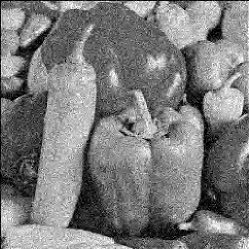
Original	Noisy	(Rissanen, 2000)
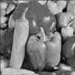
MDL (A)	MDL (A-B)	MDL (A-B-C)
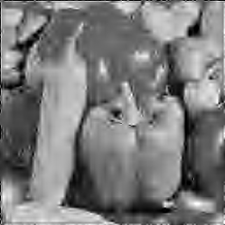
VisuShrink	SureShrink	BayesShrink

Figure 5: Simulation Results. Panels from top to bottom, left to right: Peppers image, $n=256\times 256$; noisy image, noise standard deviation $\sigma=30$, PSNR=18.6; original MDL method [23], PSNR=19.9; MDL with modification of Sec. III-A, PSNR=23.9; MDL with modifications of Secs. III-A and III-B, PSNR=24.9; MDL with modifications of Secs. III-A, III-B and III-C, PSNR=25.5; VisuShrink [8], PSNR=23.2; SureShrink [9], PSNR=24.6; BayesShrink [12], PSNR=25.9. (Higher PSNR is better).

Blocks (n=2048)

Peppers

Figure 6: Simulation Results. PSNR difference compared to the proposed method (MDL with modifications of Secs. III-A, III-B and III-C), see Figs. 4 and 5. Top row: Blocks signal [9], sample size $n=2048$. Bottom row: Peppers image, $n=256\times 256$. Left panels show the effect of each of the three modifications in Sec. III; right panels show comparison to VisuShrink [8], SureShrink [9], and BayesShrink [12].

TABLE I: Numerical Results. The peak-signal-to-noise ratio for various 1D signals, denoising methods, and noise levels. Columns: noise standard deviation $\sigma$; PSNR for different methods (see Figs. 4 and 5), best value(s) in boldface; SD: standard deviation of all PSNR’s for each value of $\sigma$ over 15 repetitions.

	(Rissanen, 2000)	MDL (A)	MDL (A-B)	MDL (A-B-C)	VisuShrink	SureShrink	BayesShrink		SD
Blocks ($n=2048$)
$\sigma=0.1$	44.4	43.8	44.5	44.9	43.6	41.9	40.1	$\pm$	0.32
0.5	28.9	29.1	30.1	30.8	29.0	29.0	30.1	$\pm$	0.42
1.0	20.4	24.4	25.5	26.2	24.3	25.2	26.1	$\pm$	0.44
1.5	15.0	21.6	22.8	23.4	21.5	22.8	23.9	$\pm$	0.34
2.0	11.7	19.6	21.6	22.2	19.5	21.6	22.6	$\pm$	0.45
Bumps ($n=2048$)
$\sigma=0.1$	39.4	39.6	40.0	40.7	39.2	38.8	38.3	$\pm$	0.38
0.5	20.6	26.8	27.8	28.4	26.1	27.2	28.0	$\pm$	0.40
1.0	13.9	21.5	23.0	23.7	21.3	23.3	24.0	$\pm$	0.30
1.5	10.3	18.6	20.6	21.3	18.9	20.5	21.9	$\pm$	0.40
2.0	7.9	17.7	19.2	19.9	17.9	19.5	20.3	$\pm$	0.38
Heavisine ($n=2048$)
$\sigma=0.1$	51.3	50.4	51.3	51.9	51.1	48.8	48.1	$\pm$	0.60
0.5	35.6	37.4	39.1	39.5	37.7	38.3	38.9	$\pm$	0.61
1.0	27.0	32.9	34.1	34.6	33.2	34.7	34.1	$\pm$	0.70
1.5	19.8	30.6	31.6	32.0	30.8	32.3	32.3	$\pm$	0.91
2.0	15.4	28.1	30.5	31.0	28.2	31.2	31.3	$\pm$	1.02
Doppler ($n=2048$)
$\sigma=0.1$	24.5	28.4	29.2	29.8	28.3	28.6	29.5	$\pm$	0.46
0.5	6.2	17.8	19.3	19.9	17.7	19.6	20.3	$\pm$	0.70
1.0	0.1	12.6	15.4	16.0	13.1	16.1	16.2	$\pm$	0.83
1.5	-3.5	10.7	13.3	13.7	10.8	14.0	13.9	$\pm$	0.75
2.0	-5.9	9.9	11.3	11.5	10.1	12.2	11.8	$\pm$	0.89

TABLE II: Numerical Results. The peak-signal-to-noise ratio for various images, denoising methods, and noise levels. Columns: noise standard deviation $\sigma$; PSNR for different methods (see Figs. 4 and 5), best value(s) in boldface; SD: standard deviation of all PSNR’s for each value of $\sigma$ over 15 repetitions.

	(Rissanen, 2000)	MDL (A)	MDL (A-B)	MDL (A-B-C)	VisuShrink	SureShrink	BayesShrink		SD
Lena ($512\times 512$)
$\sigma=0$	39.1	36.6	38.5	39.3	37.3	43.2	46.9	$\pm$	–
10	31.6	30.8	31.8	32.4	30.1	32.8	33.1	$\pm$	0.02
20	25.0	27.8	28.8	29.4	27.1	29.5	29.9	$\pm$	0.03
30	19.8	26.0	27.1	27.6	25.4	27.8	28.2	$\pm$	0.03
40	16.7	24.9	26.0	26.5	24.3	26.4	27.0	$\pm$	0.04
Boat ($512\times 512$)
$\sigma=0$	36.2	33.2	35.1	35.9	32.9	39.2	40.3	$\pm$	–
10	30.2	28.6	29.8	30.5	28.0	31.3	31.7	$\pm$	0.02
20	24.2	25.8	26.8	27.5	25.2	27.9	28.3	$\pm$	0.03
30	19.6	24.3	25.2	25.8	23.7	26.1	26.5	$\pm$	0.02
40	16.6	23.2	24.2	24.7	22.8	24.9	25.3	$\pm$	0.03
House ($256\times 256$)
$\sigma=0$	41.4	36.7	42.5	43.5	41.0	47.4	54.2	$\pm$	–
10	31.4	30.7	31.5	32.1	30.2	32.5	32.8	$\pm$	0.06
20	24.7	27.3	28.1	28.7	26.8	28.7	29.2	$\pm$	0.05
30	19.7	25.4	26.4	27.0	24.9	26.9	27.4	$\pm$	0.06
40	16.7	24.2	25.2	25.7	23.7	25.4	26.2	$\pm$	0.07
Peppers ($256\times 256$)
$\sigma=0$	38.9	36.1	37.9	38.7	36.9	42.7	51.2	$\pm$	–
10	30.7	29.3	30.3	31.0	28.6	31.5	31.5	$\pm$	0.04
20	24.7	25.9	26.9	27.6	25.1	27.1	27.9	$\pm$	0.05
30	19.9	23.9	24.9	25.5	23.1	24.6	25.9	$\pm$	0.05
40	16.8	22.4	23.3	23.9	21.6	22.8	24.4	$\pm$	0.08

V Conclusions

We have revisited an earlier MDL method for wavelet-based denoising for signals with additive Gaussian white noise. In doing so we gave an alternative interpretation of Rissanen’s renormalization technique for avoiding the problem of unbounded parametric complexity in normalized maximum likelihood (NML) codes. This new interpretation suggested three refinements to the basic MDL method which were shown to significantly improve empirical performance.

The most significant contributions are: i) an approach involving what we called the extended model, to the problem of unbounded parametric complexity which may be useful not only in the Gaussian model but, for instance, in the Poisson and geometric families of distributions with suitable prior densities for the parameters; ii) a demonstration of the importance of encoding the model index when the number of potential models is large; iii) a combination of universal models of the mixture and NML types, and a related predictive technique which should also be useful in MDL denoising methods (e.g. [20, 21, 24]) that are based on finding a single best model, and other predictive tasks.

Appendix A Postponed Proofs

Proof of Eq. (6): The proof of Eq. (6) is technically similar to the derivation of the renormalized NML model in [23], which goes back to [43]. First note that due to orthonormality, the density of $y^{n}$ under the extended model is always equal to the density of ${c}^{n}$ evaluated at ${\mathcal{W}}^{T}y^{n}$. Thus, for instance, the maximum likelihood parameters for data $y^{n}$ are easily obtained by maximizing the density of ${c}^{n}$ at ${\mathcal{W}}^{T}y^{n}$. The density of ${c}^{n}$ is given by

$$f({c}^{n}\;;\;\sigma_{I}^{2},\sigma_{N}^{2})=\prod_{i\in\gamma}\phi({c}_{i}\;;\;0,\sigma_{I}^{2})\prod_{i\notin\gamma}\phi({c}_{i}\;;\;0,\sigma_{N}^{2}),$$ (13)

where $\phi(\cdot\;;\;\mu,\sigma^{2})$ denotes a Gaussian density function with mean $\mu$ and variance $\sigma^{2}$.

Let $S_{\gamma}(y^{n})$ be the sum of squares of the wavelet coefficients with $i\in\gamma$:

$$S_{\gamma}(y^{n}):=\sum_{i\in\gamma}{c}_{i}^{2}.$$

and let $S(y^{n})$ denote the sum of all wavelet coefficients. With slight abuse of notation, we also denote these two by $S_{\gamma}({c}^{n})$ and $S({c}^{n})$, respectively. Let $k$ be the size of the set $\gamma$.

The likelihood is maximized by parameters given by

$$\hat{\sigma}_{I}^{2}=\frac{S_{\gamma}(y^{n})}{k},\quad\hat{\sigma}_{N}^{2}=\frac{S(y^{n})-S_{\gamma}(y^{n})}{n-k}.$$ (14)

With the maximum likelihood parameters (14) the likelihood (13) becomes

$$(2\pi e)^{-n/2}\left(\frac{S_{\gamma}(y^{n})}{k}\right)^{-k/2}\left(\frac{S(y^{n})-S_{\gamma}(y^{n})}{n-k}\right)^{-\frac{n-k}{2}}.$$ (15)

The normalization constant $C$ is also easier to evaluate by integrating the likelihood in terms of ${c}^{n}$:

$$C =A\int\left(S_{\gamma}({c}^{n})\right)^{-k/2}\left(S({c}^{n})-S_{\gamma}({c}^{n})\right)^{-\frac{n-k}{2}}\,d{c}^{n},$$ (16)

where $A$ is given by

$$A=(2\pi e)^{-n/2}k^{k/2}(n-k)^{\frac{n-k}{2}},$$

and the range of integration $R$ is defined by requiring that the maximum likelihood estimators (14) are both within the interval $[\sigma^{2}_{\min},\sigma^{2}_{\max}]$. It will be seen that the integral diverges without these bounds. The integral factors in two parts involving only the coefficients with $i\in\gamma$ and $i\notin\gamma$ respectively. Furthermore, the resulting two integrals depend on the coefficients only through the values $S_{\gamma}({c}^{n})$ and $S({c}^{n})-S_{\gamma}({c}^{n})$, and thus, they can be expressed in terms of these two quantities as the integration variables – we denote them respectively by $s_{1}$ and $s_{2}$. The associated Riemannian volume elements are infinitesimally thin spherical shells (surfaces of balls); the first one with dimension $k$ and radius $s_{1}^{1/2}$, the second one with dimension $n-k$ and radius $s_{2}^{1/2}$, given by

$$\frac{\pi^{k/2}s_{1}^{k/2-1}}{\Gamma(k/2)}\,ds_{1},\quad\frac{\pi^{(n-k)/2}s_{2}^{(n-k)/2-1}}{\Gamma((n-k)/2)}\,ds_{2}.$$

Thus the integral in (16) is equivalent to

$$\int_{k\sigma^{2}_{\min}}^{k\sigma^{2}_{\max}}\frac{\pi^{k/2}s_{1}^{k/2-1}}{\Gamma(k/2)}s_{1}^{-k/2}\,ds_{1}\\ \times\int_{(n-k)\sigma^{2}_{\min}}^{(n-k)\sigma^{2}_{\max}}\frac{\pi^{(n-k)/2}s_{2}^{(n-k)/2-1}}{\Gamma((n-k)/2)}s_{2}^{-(n-k)/2}\,ds_{2}.$$ (17)

Both integrands become simply of the form $1/x$ and hence, the value of the integral is given by

$$\frac{\pi^{n/2}}{\Gamma(k/2)\Gamma((n-k)/2)}\left(\ln\frac{\sigma^{2}_{\max}}{\sigma^{2}_{\min}}\right)^{2},$$ (18)

Plugging (18) into (16) gives the value of the normalization constant

$$C=\frac{k^{k/2}(n-k)^{(n-k)/2}}{(2e)^{n/2}\Gamma(k/2)\Gamma((n-k)/2)}\left(\ln\frac{\sigma^{2}_{\max}}{\sigma^{2}_{\min}}\right)^{2}.$$

Normalizing the numerator (15) by $C$, and canceling like terms finally gives the NML density:

$$f_{{\text{\emph{nml}}}}(y^{n})=\frac{\Gamma(k/2)\Gamma((n-k)/2)}{\pi^{n/2}(S_{\gamma}(y^{n}))^{k/2}(S(y^{n})-S_{\gamma}(y^{n}))^{(n-k)/2}}\\ \times\left(\ln\frac{\sigma^{2}_{\max}}{\sigma^{2}_{\min}}\right)^{-2},$$ (19)

and the corresponding code length becomes

$$-\ln f_{{\text{\emph{nml}}}}(y^{n}) =\frac{k}{2}\ln S_{\gamma}(y^{n})+\frac{n-k}{2}\ln(S(y^{n})-S_{\gamma}(y^{n}))$$

$$-\ln\Gamma\left(\frac{k}{2}\right)-\ln\Gamma\left(\frac{n-k}{2}\right)$$

$$+\frac{n}{2}\ln\pi+2\ln\ln\frac{\sigma^{2}_{\max}}{\sigma^{2}_{\min}}.$$

Applying Stirling’s approximation

$$\ln\Gamma(z)\approx\left(z-\frac{1}{2}\right)\ln z-z+\frac{1}{2}\ln 2\pi,$$

to the Gamma functions yields now

$$-\ln f_{\text{\emph{nml}}}(y^{n}) \approx\frac{k}{2}\ln S_{\gamma}(y^{n})+\frac{n-k}{2}\ln(S(y^{n})-S_{\gamma}(y^{n}))$$

$$-\left(\frac{k-1}{2}\right)\ln\left(\frac{k}{2}\right)+\frac{k}{2}$$

$$-\left(\frac{n-k-1}{2}\right)\ln\left(\frac{n-k}{2}\right)+\frac{n-k}{2}$$

$$-\ln 2\pi+\frac{n}{2}\ln\pi+2\ln\ln\frac{\sigma^{2}_{\max}}{\sigma^{2}_{\min}}.$$

Rearranging the terms gives the formula

$$-\ln f_{\text{\emph{nml}}}(y^{n})\approx\frac{k}{2}\ln\frac{S_{\gamma}(y^{n})}{k}+\frac{n-k}{2}\ln\frac{S(y^{n})-S_{\gamma}(y^{n})}{n-k}\\ +\frac{1}{2}\ln k(n-k)+\text{\emph{const}},$$ (20)

where const is a constant wrt. $\gamma$, given by

$$\text{\emph{const}}=\frac{n}{2}\ln 2\pi e-\ln 4\pi+2\ln\ln\frac{\sigma^{2}_{\max}}{\sigma^{2}_{\min}}.$$

∎

Proof of Proposition 1: The maximum likelihood parameters (14) may violate the restriction $\sigma_{I}^{2}\geq\sigma_{N}^{2}$ that arises from the definition $\sigma_{I}^{2}{\;:=\;}\tau^{2}+\sigma_{N}^{2}$. The restriction affects range of integration in Eq. (18) giving the non-constant terms as follows

$$\int_{k\sigma_{\min}^{2}}^{k\sigma_{\max}^{2}}\left(\int_{(n-k)\sigma_{\min}^{2}}^{((n-k)/k)s_{1}}s_{1}^{-1}s_{2}^{-1}\,ds_{2}\right)\,ds_{1}\\ =\int_{k\sigma_{\min}^{2}}^{k\sigma_{\max}^{2}}s_{1}^{-1}(\ln s_{1}-\ln k\sigma_{\min}^{2})\,ds_{1}.$$ (21)

Using the integral $\int s_{1}^{-1}\ln s_{1}\,ds_{1}=\frac{1}{2}(\ln s_{1})^{2}$ gives then

$$\frac{1}{2}(\ln k\sigma_{\max}^{2})^{2}-\frac{1}{2}(\ln k\sigma_{\min}^{2})^{2}-\ln k\sigma_{\min}^{2}\left(\ln\frac{\sigma_{\max}^{2}}{\sigma_{\min}^{2}}\right),$$ (22)

where the first two terms can be written as

$$\frac{1}{2}\left(\ln k\sigma_{\max}^{2}+\ln k\sigma_{\min}^{2}\right)\left(\ln\frac{\sigma_{\max}^{2}}{\sigma_{\min}^{2}}\right).$$

Combining with the third term of (22) changes the plus into a minus and gives finally

$$\frac{1}{2}\left(\ln\frac{\sigma_{\max}^{2}}{\sigma_{\min}^{2}}\right)\left(\ln\frac{\sigma_{\max}^{2}}{\sigma_{\min}^{2}}\right),$$

which is exactly half of the integral in Eq. (18), the constant terms being the same. Thus, the effect of the restriction on the code length where the logarithm of the integral is taken, is one bit, i.e., $\ln 2$ nats.

∎

Proof of Eq. 8: The relevant terms in the code length $\ln{n\choose k}$, i.e. those depending on $k$, for the index of the model class are

$$-\ln(k!(n-k)!) =-\ln[k(k-1)!(n-k)(n-k)!]$$

$$=-\ln(k(n-k))-\ln\Gamma(k)-\ln\Gamma(n-k),$$

which gives after Stirling’s approximation (ignoring constant terms)

$$-\ln(k(n-k))-\left(k-\frac{1}{2}\right)\ln k+k\\ -\left(n-k-\frac{1}{2}\right)\ln(n-k)+(n-k)\\ =-\frac{k}{2}\ln k^{2}-\frac{n-k}{2}\ln(n-k)^{2}+\frac{1}{2}\ln k(n-k)+n.$$ (23)

Adding this to Eq. 6 (without the constant $n$) gives Eq. (8).

∎

References

- [1] S. Mallat, A Wavelet Tour of Signal Processing. Academic Press, 1998.
- [2] ——, “A theory for multiresolution signal decomposition: the wavelet representation,” IEEE Trans. Pattern Analysis and Machine Intelligence, vol. 11, pp. 674–693, 1989.
- [3] R. A. DeVore, B. Jawerth, and B. J. Lucier, “Image compression through wavelet transform coding,” IEEE Trans. Information Theory, vol. 38, no. 2, pp. 719–746, Mar. 1992.
- [4] J. Villasenor, B. Belzer, and J. Liao, “Wavelet filter evaluation for image compression,” IEEE Trans. Image Processing, vol. 4, no. 8, pp. 1053–1060, Aug. 1995.
- [5] B. K. Natarajan, “Filtering random noise from deterministic signals via data compression,” IEEE Trans. Information Theory, vol. 43, no. 11, pp. 2595–2605, Nov. 1995.
- [6] M. Hansen and B. Yu, “Wavelet thresholding via MDL for natural images,” IEEE Trans. Information Theory (Special Issue on Information Theoretic Imaging), vol. 46, pp. 1778–1788, 2000.
- [7] J. Liu and P. Moulin, “Complexity-regularized image denoising,” IEEE Trans. Image Processing, vol. 10, no. 6, pp. 841–851, June 2001.
- [8] D. Donoho and I. Johnstone, “Ideal spatial adaptation via wavelet shrinkage,” Biometrika, vol. 81, pp. 425–455, 1994.
- [9] ——, “Adapting to unknown smoothness via wavelet shrinkage,” J. Amer. Statist. Assoc., vol. 90, no. 432, pp. 1200–1224, 1995.
- [10] B. Vidakovic, “Nonlinear wavelet shrinkage with Bayes rules and Bayes factors,” J. Amer. Statist. Assoc., vol. 93, no. 441, pp. 173–179, 1998.
- [11] F. Ruggeri and B. Vidakovic, “A Bayesian decision theoretic approach to the choice of thresholding parameter,” Statistica Sinica, vol. 9, pp. 183–197, 1999.
- [12] G. Chang, B. Yu, and M. Vetterli, “Adaptive wavelet thresholding for image denoising and compression,” IEEE Trans. Image Proc., vol. 9, pp. 1532–1546, 2000.
- [13] P. Moulin and J. Liu, “Analysis of multiresolution image denoising schemes using generalized Gaussian and complexity priors,” IEEE Trans. Information Theory, vol. 45, no. 3, pp. 909–919, Apr. 1999.
- [14] M. Wainwright and E. Simoncelli, “Scale mixtures of Gaussians and the statistics of natural images,” in Advances in Neural Information Processing Systems, S. Solla, T. Leen, and K.-R. Muller, Eds., vol. 12. MIT Press, May 2000, pp. 855–861.
- [15] J. Portilla, V. Strela, M. Wainwright, and E. Simoncelli, “Image denoising using scale mixtures of Gaussians in the wavelet domain,” IEEE Trans. Image Processing, vol. 12, no. 11, pp. 1338–1351, Nov. 2003.
- [16] J. Rissanen, “Modeling by shortest data description,” Automatica, vol. 14, pp. 445–471, 1978.
- [17] ——, “Fisher information and stochastic complexity,” IEEE Trans. Information Theory, vol. 42, no. 1, pp. 40–47, January 1996.
- [18] P. Grünwald, “A Tutorial introduction to the minimum description length principle,” in Advances in MDL: Theory and Applications, P. Grünwald, I. Myung, and M. Pitt, Eds. MIT Press, 2005.
- [19] ——, The Minimum Description Length Principle. MIT Press, forthcoming.
- [20] N. Saito, “Simultaneous noise suppression and signal compression using a library of orthonormal bases and the minimum description length criterion,” in Wavelets in Geophysics. Academic Press, 1994, pp. 299–324.
- [21] A. Antoniadis, I. Gijbels, and G. Gregoire, “Model selection using wavelet decomposition and applications,” Biometrika, vol. 84, no. 4, pp. 751–763, 1997.
- [22] H. Krim and I. Schick, “Minimax decription length for signal denoising and optimized representation,” IEEE Trans. Information Theory, vol. 45, no. 3, pp. 898–908, 1999.
- [23] J. Rissanen, “MDL denoising,” IEEE Trans. Information Theory, vol. 46, no. 7, pp. 2537–2543, 2000.
- [24] V. Kumar, J. Heikkonen, J. Rissanen, and K. Kaski, “Minimum description length denoising with histogram models,” IEEE Trans. Signal Processing, vol. 54, no. 8, pp. 2922–2928, 2006.
- [25] I. Daubechies, Ten Lectures on Wavelets. Society for Industrial & Applied Mathematics (SIAM), 1992.
- [26] D. Foster and R. Stine, “The competitive complexity ratio,” in Proc. 2001 Conf. on Information Sciences and Systems, 2001, pp. 1–6.
- [27] ——, “The contribution of parameters to stochastic complexity,” in Advances in MDL: Theory and Applications, P. Grünwald, I. Myung, and M. Pitt, Eds. MIT Press, 2005.
- [28] F. Liang and A. Barron, “Exact minimax strategies for predictive density estimation, data compression, and model selection,” IEEE Trans. Information Theory, vol. 50, no. 11, pp. 2708–2726, Nov. 2004.
- [29] S. de Rooij and P. Grünwald, “An empirical study of MDL model selection with infinite parametric complexity,” J. Mathematical Psychology, vol. 50, no. 2, pp. 149–166, 2006.
- [30] T. Roos, P. Myllymäki, and H. Tirri, “On the behavior of MDL denoising,” in Proc. Tenth Int. Workshop on AI and Stat., R. G. Cowell and Z. Ghahramani, Eds. Society for AI and Statistics, 2005, pp. 309–316.
- [31] T. J. Mitchell and J. J. Beauchamp, “Bayesian variable selection in linear regression (with discussion),” J. Amer. Statist. Assoc., vol. 83, no. 404, pp. 1023–1032, Dec. 1988.
- [32] E. I. George and R. E. McCulloch, “Approaches for Bayesian variable selection,” Statistica Sinica, vol. 7, no. 2, pp. 339–374, 1997.
- [33] H. A. Chipman, E. D. Kolaczyk, and R. E. McCulloch, “Adaptive Bayesian wavelet shrinkage,” J. Amer. Statist. Assoc., vol. 92, no. 440, pp. 1413–1421, 1997.
- [34] F. Abramovich, T. Sapatinas, and B. Silverman, “Wavelet thresholding via a Bayesian approach,” J. Royal Statist. Soc. Series B, vol. 60, no. 4, pp. 725–749, 1998.
- [35] P. Kontkanen, P. Myllymäki, W. Buntine, J. Rissanen, and H. Tirri, “An MDL framework for data clustering,” in Advances in MDL: Theory and Applications, P. Grünwald, I. Myung, and M. Pitt, Eds. MIT Press, 2005.
- [36] J. Rissanen, “Strong optimality of the normalized ML models as universal codes and information in data,” IEEE Trans. Information Theory, vol. 47, no. 5, pp. 1712–1717, 2001.
- [37] Y. Shtarkov, “Universal sequential coding of single messages,” Problems of Information Transmission, vol. 23, pp. 175–186, 1987.
- [38] J. Rissanen, “Lectures on statistical modeling theory,” Aug. 2005, available at http://www.mdl-research.org/.
- [39] J. Ojanen, T. Miettinen, J. Heikkonen, and J. Rissanen, “Robust denoising of electrophoresis and mass spectrometry signals with minimum description length principle,” FEBS Letters, vol. 570, no. 1–3, pp. 107–113, 2004.
- [40] I. Csiszár and P. Shields, “The consistency of the BIC Markov order estimator,” Annals of Statistics, vol. 28, pp. 1601–1619, 2000.
- [41] N. Vereshchagin and P. Vitányi, “Kolmogorov’s structure functions and model selection,” IEEE Trans. Information Theory, no. 12, pp. 3265–3290, Dec. 2004.
- [42] F. Willems, Y. Shtarkov, and T. Tjalkens, “The context-tree weighting method: basic properties,” IEEE Trans. Information Theory, vol. 41, no. 3, pp. 653–664, 1995.
- [43] B. Dom, “MDL estimation for small sample sizes and its application to linear regression,” IBM Research, Tech. Rep. RJ 10030, 1996.