One approach to the digital visualization
of hedgehogs in holomorphic dynamics

Abstract

In the field of holomorphic dynamics in one complex variable, hedgehog is the local invariant set arising about a Cremer point and endowed with a very complicate shape as well as relating to very weak numerical conditions. We give a solution to the open problem of its digital visualization, featuring either a time saving approach and a far-reaching insight.

1 Introduction

Let ${\mathbb{C}}$ be the complex plane. Since $\infty$ cannot be handled like an ordinary point here, as deserved by many complex functions, this lack is fulfilled by the compactification ${\mathbb{C}}_{\infty}={\mathbb{C}}\cup\{\infty\}$, namely the extended complex plane; anyway the representation of the neighborhood of $\infty$ is still impracticable here. Riemann cracked the problem by a stereographic projection of ${\mathbb{C}}_{\infty}$ onto a sphere of radius 1: this is the Riemann sphere $\hat{{\mathbb{C}}}$.

Holomorphic dynamics collect the studies on the iterates $f_{n}$ of the function $f:{\mathbb{C}}_{\infty}^{v}\rightarrow{\mathbb{C}}_{\infty}^{v}$ of given type (entire, meromorphic, transcendental, …) and in one or several complex variables (depending on $v\geq 1$). The map $f$ is of finite degree.

We will deal with the case of one variable, where $v=1$. The questions in this field may rise to high degrees of complication and many ones deserve a multilateral attack rooting into Complex Analysis, Topology, Theory of Numbers, Uniformization Theory. One of the most important goals is the study of elements not changing under iteration: the so-called invariants, showing up to dimension $2$ at most: they might be points (dim 0), lines (dim 1) or surfaces (dim 2). The collection of invariants with a same property is the invariant set.

It is convenient to split results into the ‘local’ and into the ‘global’ branch, in order to have a good picture of the whole corpus. A local study investigates on the properties which hold up to a finite distance from the invariant set, thus inside a bounded domain; while a global approach wants those properties enjoyed by points being even at infinite distance, thus all over the $\hat{{\mathbb{C}}}$. Branches are not disjoint and related concepts act in mutual cooperation: in fact, either locally or globally, the fate of (inverse and forward) orbits closely relates to the nature of the fixed point $\delta$ and its neighborhood.

Results rely on the study of the orbits, i.e. the set of points generated by iterating the given function $f$,

$$f_{1}\equiv f,f_{2}\equiv f[f],\dots,\ f_{n}\equiv f[f_{n-1}].$$

approaching to limit sets which may consist of finitely (dim 0), or of infinitely and uncountably many (dim 1 and 2) points. For such sets finitely many points of order $k>1$, one speaks of limit cycle of periodic points $\delta_{n}$:

$$f(\delta_{1})=\delta_{2},f(\delta_{2})=\delta_{3},\dots,f(\delta_{k-1})=\delta_{1}.$$ (1.1)

If the period is $k\geq 1$, then $\delta_{1\leq i\leq k}=f_{k}(\delta_{1\leq i\leq k})$. If $k=1$, we have the limit fixed point $\delta$ and the expression (1.1) boils down to:

$$\delta=f(\delta).$$ (1.2)

so the fixed point can be re-framed as a cycle of period $1$.

Other cycles may belong to invariants $J$ of dimension 0 (infinitely many points), or 1 and, exceptionally, of dimension 2 (both, uncountably many).

In the economy of dynamics over $\hat{{\mathbb{C}}}$, cycles of finitely or of infinitely and of uncountably many points play different roles which are explained locally in the former case, while the latter cycles are object of the global investigation.

In the second case, we speak of ‘Julia sets’ $J$: when they include infinitely many points, their topology is totally disconnected; when uncountably many, they are continuous (Jordan curves or not).

With the caution to the casuistry of related local dynamics, a same limit cycle of finitely many points groups all orbits converging to it into macro-sets, said ‘the basins $\mathcal{B}$ of attraction’, also defined ‘Fatou sets’, in honor of Pierre Fatou (1878–1929), who co-pioneered these investigations in the same times (1918–20) and independently from Gaston Julia (1893–1978), who is credited as the first official discoverer of sets $J$ in 1918. While the role of the basins is to include all those orbits to a same limit cycle, $J$ is the boundary between the basins.

Julia sets are well-known objects at all levels today, sparkling the imagination a wide range of people, from artists to mathematicians. The details of their suggestive and very complicated fractal shapes were disclosed to human eyes by the early computer experiments during late 1970s: machines revealed to be the indispensable aid for overcoming the long standing barriers of hand-written, rough plots available to those ancient mathematicians. The technologic run is continuously opening to finer results, thanks to higher screen resolutions and faster CPU saving from long time consuming computations, as required to render these images. Anyway this side role shows that Technology is not a priority and does not fully belong to the road-map of this field: it is just a good tool to develop those methods mastering both analytical and geometrical relations – which are most wanted today –, together with more accurate numerical precision, especially for the question we are going to deal with.

Even at the graphical level, we differ local from global methods, whether they focus on the previous limit sets related to the two branches.

After some introductory theory culminating into the presentation of what the invariant sets $\mathcal{H}$, said ‘hedgehogs’, are meant in holomorphic dynamics, we will illustrate the related problem by showing how most available techniques fail to display $\mathcal{H}$ adequately; finally, we will discuss how to solve this question and to code an approach via pseudo-C${}^{\textnormal{++}}$ language code.

2 Basic theory

2.1 The four cases

We are going to sketch out the mathematical terms of our local environment: here complex dynamics are mostly interested in the orbits behavior induced by iterates $f_{n}(z)$ near limit cycles of the map $f$ and focuses on cycles of order 1, i.e. fixed points $\delta,f(\delta)=\delta$. For an easier approach, we will assume fixed points from now on. Iterates are operators defined as follows in the forward sense ($n\geq 0$):

$$f_{0}(z)\equiv z,f_{1}(z)\equiv f(z),f_{2}(z)\equiv f[f(z)],\dots\ ,f_{n}(z)\equiv f[f_{n-1}(z)];$$

or backwards by a composition of inverse maps ($n<0$):

$$f_{-1}(z)\equiv f^{-1}(z),f_{-2}(z)\equiv f^{-1}[f^{-1}(z)],\dots\ .$$

The starting point $z$ of an orbit is said the seed.

The classification of $\delta$ is achieved by computing the modulus $\lambda$ of the first derivative $f^{\prime}$ at $\delta$, $\lambda=|f^{\prime}(\delta)|$ and it is essential to understand the nature of local invariant sets, grouped here into four main classes:

1. super-attracting fixed point, when $|\lambda|=0$;

2. attracting fixed point, when $0<|\lambda|<1$;

3. indifferent or neutral fixed point, when $|\lambda|=1=|e^{2\pi i\theta}|$;

4. repelling fixed point, when $|\lambda|>0$;

Reader’s understanding can be lessened by splitting this basic classification into two extremal cases, (super–)attracting and repelling entries, their directions are opposite but dynamical properties are very similar. With it, one understand that the indifferent case stands at the middle way and it is the conjunction point among those ones, either in a inclusive way by presenting subcases where all dynamical features are shown at the same time and in an exclusive way, i.e. showing features which are not enjoyed by both extremal cases.

In fact (super–)attracting fixed points can be reached by forward iterates, whereas Julia sets include cycles of repelling points and reached by backward iterates. Obviously, the dynamical characters (contraction, repulsion) of entries 1), 2) and 4) hold for the direct function $f(z)$, while they are inverted for $f^{-1}(z)$. Indifferent points deserve a separate discussion, where even the concept of ‘limit’ shall be carefully applied, because not conventionally intended like in the other cases.

While entries 1), 2) and 4) just need the modulus value, case 3) requires a thorough investigation: the modulus is insufficient to distinguish the more complex casuistry here, as illustrated in table 2.1; another parameter is demanded and our next (and immediate) choice is the angle $0\leq\theta<2\pi,\theta\in{\mathbb{R}}$. Its numerical properties rule out the dynamical characters of neighboring orbits about indifferent points. The main separation, into the two great classes of $\theta\in{\mathbb{Q}}$ (rationally indifferent $\delta$, parabolic case) and of $\theta\in{\mathbb{R}}\backslash{\mathbb{Q}}$ (irrationally indifferent $\delta$, elliptic case), is followed by a number of sub-cases. The former relates to one only invariant set, namely the Fatou-Leau flower (see def. at p. 5.1), and does not branch out; while $\theta\in{\mathbb{R}}\backslash{\mathbb{Q}}$ generates a richer variety whose local dynamics get far more complicate: here a second level opens to local invariant sets, distinguishing for the numerical properties of $\theta$, some of which are extremely weak and shunning the machine finite digits computation. The goal of this work is understand how and if such latter cases might be actually attackable in particular graphical terms which evince their local dynamics.

2.2 Analogy with linear models

One crucial tool to study the local dynamics is the Schröder functional equation (SFE):

$$\psi[f(z)]=a[\psi(z)],$$ (2.1)

where $\psi(z)$ is an invertible map. Without loss of generalization, let the origin be fixed for $f$. If we replace $a(z)$ with $\lambda\equiv f^{\prime}(z)$ – the meaning of the first derivative strengthens the application of SFE to local problems, then (2.1) turns into this version:

$$\psi[f(z)]=\lambda\psi(z).$$ (2.2)

Given a sufficiently close neighborhood $D$ of $\delta$, the left diagram below, as well as the right one extending to iterates, commutes when SFE holds:

$D$	$\xrightarrow{}$	$f(D)$		$D$	$\xrightarrow{}$	$f^{n}(D)$
$\psi\downarrow$		$\psi\downarrow$		$\psi\downarrow$		$\psi\downarrow$
${\mathbb{C}}_{\infty}$	$\xrightarrow{\lambda}$	${\mathbb{C}}_{\infty}$		${\mathbb{C}}_{\infty}$	$\xrightarrow{\lambda^{n}}$	${\mathbb{C}}_{\infty}$

The major goal of (2.2) is to set up an analogy between the behavior of iterates $f_{n}(z)$ about $\delta$ and an easier model; so, if SFE commutes, there is a local change of coordinates where $f(0)=0,f^{\prime}(z)=\lambda$: the local behavior of orbits $f_{n}(z)$ can be studied by means of the simpler investigation of the linear map $\lambda^{n}z$.

0.9 normal

Table 2.1 : Resuming the neutrality. A diagram illustrating the classification of all dynamics for indifferent fixed points.

Local theory had proven that SFE holds only for the (super–)attracting and the repelling case, together with the rationally indifferent and part of the irrationally indifferent cases (see list at p. 2.1). If the local change of coordinates into $\lambda z$ applies, $D$ is a Böttcher or a Koenigs’ domain, depending on $\lambda=0$ and $\lambda<1$ respectively. For $\lambda>1$, local dynamics are repelling and, locally speaking exclusively, this case can be regarded as the converse of the attracting one; anyway here Fatou and Julia showed that it makes more sense of studying repelling orbits and the related invariant set (as resumed in diagram 2.2) in global terms: this is the Julia set, defined as the closure of all repelling cycles and being the common frontier of all basins $\mathcal{B}$ of convergence.

0.8 normal

Table 2.2 : Classification by motions. This is the classification of invariant sets for holomorphic dynamics in one complex variable by the three elementary motions in the plane.

The discussion of $|\lambda|=1$ requires a much more delicate analysis: first, its re-writing in the formal terms of (2.2) is

$$\psi[f(z)]=e^{2\pi i\theta}\psi(z)\quad\Rightarrow\quad\psi[f_{n}(z)]=e^{2\pi i\theta n}\psi(z),$$ (2.3)

where the version on the right refers to iterates $f_{n}(z)$, conjugated locally to the family of complex rotations $e^{2\pi\theta in}z$. Problems arose when it was seen that (2.3) does not always commute, given $\theta\in{\mathbb{R}}$, whether it does or not is up to the numerical nature of $\theta$. For example, it never commutes for $\theta\in{\mathbb{Q}}$, while it does when $\theta\in{\mathbb{R}}\backslash{\mathbb{Q}}$ satisfies this Diophantine condition: given two numbers $r>0,k\geq 2$,

$$|\theta-p/q|>r/q^{k},$$ (2.4)

for every rational number $p/q$ where $p,q\in{\mathbb{N}}$. Then $f_{n}(z)$ are said to be linearizable into a complex rigid rotation or, simply, ‘linearizable’; topologically speaking, there exists a neighborhood of $\delta$ which is conformally isomorphic to a disc and where the dynamics of $f_{n}(z)$ are rotational, the Siegel disc. When (2.4) holds, $\theta$ is poorly approximated by rational numbers; otherwise it is goodly approximated. It is clear that rational numbers (parabolic sub-case, $\theta\in{\mathbb{Q}}$) are not Diophantine, together with a subclass of irrationals $\theta$, the Liouville numbers – not satisfying (2.4). In both cases, SFE fails and quits to be useful for investigations, whose achievement shall necessarily rely on other tools. Therefore one summarizes the previous concepts as follows:

$\bullet$ when SFE commutes in a sufficiently close neighborhood of (super–)attracting, indifferent and repelling points, the local behavior of iterates links to only one among the three elementary motions (either contraction, rotation, repulsion respectively) [] with regard to the fixed point $\delta$; elementary motions also include the translation $f(z):z+k$ and the identity map $f(z):z$, known to apply at the fixed points.

$\bullet$ so SFE classifies orbits dynamics by contraction, rotation, repulsion exclusively; it turns out that, as SFE fails, local dynamics do not involve only one elementary motions, as explained in diagram 2.2: then Fatou-Leau flowers and Hedgehogs consist of compositions of more than one elementary motion. Hence the failure of SFE shuts the door to linearizability.

2.3 Hedgehogs, the next stop

Stepping in the second sub-level of table 2.1, we assume to deal with holomorphic quadratic germ

$$f(z):e^{2\pi i\theta}z+z^{2}+\dots\ .$$ (2.5)

Iterates $f_{n}(z)$ can be thus expressed in this form:

$$f_{n}(z):e^{2\pi i\theta n}z+\mathcal{O}(z^{k}),\qquad n\geq 1,k\geq 2$$ (2.6)

If compared to (2.3), the question boils down to the study of the $\theta$ values so that $\mathcal{O}(z^{k})$ vanishes or not, together with the related topological dynamics. It is straight-forward that $\mathcal{O}(z^{k})=0$ allows to conjugate locally the iterations to the rigid and aperiodic rotation $f_{n}(z):e^{2\pi i\theta n}z$ (fig. 2.3/A) in a sufficiently close neighborhood of $\delta$. Topologically speaking, if $\theta$ enjoys the diophantine condition (2.4), the invariant set is a disc-shaped neighborhood, the Siegel disc $\mathcal{S}$ centered at $\delta$, which Julia termed center like Poincaré did for the analogous points in the field of differential equations:

Definition 2.1 (Siegel Disc)

Let $f$ be a non-linear complex function (2.5) and let $\delta$ be an irrationally indifferent fixed point, so that $|f^{\prime}(\delta)|=e^{2\pi i\theta}$. If $\theta$ enjoys the diophantine condition (2.4), the SFE (2.3) commutes and there exists a sufficiently close neighborhood $\mathcal{S}$ of $\delta$, so that $\mathcal{S}$ is a simply connected component of the basin and analytically conjugated to an aperiodic rotation $e^{2\pi i\theta}$ of the unit disc ${\mathbb{D}}$. ([11], p. 117)

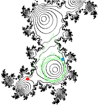
0.8normal

Figure 2.1 : Singular dynamics. Tracking down one orbit inside the basin of attraction with a Siegel disc $\mathcal{S}$. The red and blue points mark the seed $z$ and the final iterated image point $z_{n}$ respectively. This figure was plot by nested circles equi-potentials.

What happens if this condition is no longer met by $\theta\in{\mathbb{R}}\backslash{\mathbb{Q}}$? Recent Mathematics has been stressing that the concept of ‘Natura non facit saltus’ rules out for dynamical systems. Researches ([6, 14, 19, 20], to quote a few) showed the existence of irrationals $\theta$ dropping gradually off the diophantine condition (2.4): the Siegel disc $\mathcal{S}$ slowly turns into a new topological family of invariant sets, namely the hedgehogs $\mathcal{H}$. We cannot expect immediate changes in the local geometry: $\mathcal{S}$ squeezes into a smaller disc and neighboring orbits inside $\mathcal{B}\backslash\mathcal{S}$ get very complicated; if $\mathcal{S}$ is not maximal, we say that $\mathcal{H}$ has a small linearization area. In fact, with regard of the angle value $\theta$ involved, $\mathcal{S}$ may shrink to the fixed point $\delta$: here $\mathcal{H}$ has no linearization area and $\delta$ is defined a Cremer point.

During 1920s and 30s, Cremer showed [7] that the set ${\mathbb{R}}\backslash{\mathbb{Q}}$ of all irrationals can be partitioned into two disjoint subsets, $\mathcal{M},\mathcal{N}$:

$\bullet$ let $\mathcal{M}$ be the set of angles $\theta$ so that $\mathcal{D}_{c}$ is enjoyed, then a maximal Siegel disc $\mathcal{S}$ exists; $\mathcal{M}$ is a full Lebesgue’s measure set;

$\bullet$ let $\zeta\in\mathcal{N}$ be angles whose value is a Liouville number. $\mathcal{N}$ is a null-measure set.

In the course of his proof on the existence of non-centers for rational maps [7], Cremer also showed that the iterates $R^{n}(z)$ give rise to periodic cycles of growing order $n$ in the neighborhood of the non-linearizable indifferent $\delta$. He also found that they accumulate at $\delta$ while

$$\liminf_{n=1,2,\dots}\sqrt[s^{n}]{|\beta^{n}-1|}=0$$ (2.7)

which holds for

$$\liminf_{n=1,2,\dots}|\beta^{n}-1|=0\qquad\textnormal{\footnotesize\em and}\qquad\liminf_{n=1,2,\dots}\beta^{n}=1,\beta=e^{2\pi i\theta}.$$ (2.8)

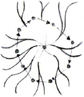
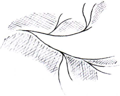
(A)	(B)

0.9normal

Figure 2.2 : Wedging the bounded basin (I) Two hand-made drawings of the hedgehog entering the bounded basin (shaded region). The wedging white region is the basin of the point at infinity.

Since the number of (super–)attracting cycles is finite (according to Koenigs’ conjecture in 1883 and proved to hold by Fatou and Julia) and the Julia set $J$ nature (closure of repelling cycles), most of the periodic points in these cycles have to be repelling so that, roughly speaking, [6] their accumulation shows that, as $n$ grows, $J$ wedges (see figs. 2.3 and 5.8) the bounded basin of attraction: if $n$ has no upper bound, then $\delta\in J$, otherwise the wedging action of $J$ stops at a certain distance from $\delta$ for $n\rightarrow K<+\infty$. The zero limit in (2.7) is reached when $\alpha$ is rational or it is a Liouville number; hence a poorly rational approximation – for the diophantine condition for $\theta$ – implies rotation around $\delta$, because cycles do not accumulate at it.

& (A) (B) (C) (D) 0.9normal Inspired by continuity, it is suggestive to think of arranging an ideal journey, along the number properties so to visit all invariant sets arising for indifferent fixed point, from (A) to (D), that is, numerically speaking in terms of $\theta$, from ${\mathbb{R}}\backslash{\mathbb{Q}}$ to ${\mathbb{Q}}$. During the journey, the Siegel disc $\mathcal{S}$ squeezes (fig. 2.3/B) until it disappears (fig. 2.3/C); for both cases B and C, the invariant sets are ‘hedgehogs’ $\mathcal{H}$, when $\mathcal{S}$ is not maximal or has empty interior. This additional look-up at the journey is inspired by the strong unifying power offered by hedgehogs theory, which links apparently far dynamical configurations. The mathematical definition of the hedgehog $\mathcal{H}$ is [14] as follows:

Definition 2.2 (Hedgehog)

Given a neighborhood $U$of an irrationally indifferent point $\delta$, so that the holomorphic map $f$ is univalent on $U$, the hedgehog $\mathcal{H}isaninvariantcompactum$, so that $f$ is not linearizable or has linearization domain relatively compact in $U$.

Figure 2.3 : The ideal journey. Simple figures of the local invariant sets related to the numerical properties of the angle $\theta$ for indifferent points: from the Siegel disc (A) to a Fatou-Leau flower (D).

Figure 2.4 : Hedgehogs generation. An illustration of $3$ steps (different shades of grey) of repelling cycles accumulation. The starred-shape, due to the cycles getting near $\delta$, as well as wedging action of the Julia set $J$, are evident.

0.7normal

For (2.5), the current research investigates on the semi–local dynamics about $\mathcal{H}$ and thanks to the results by Pérez-Marco in 1990 ([11], p. 123) one knows that $\mathcal{H}$ may show up in these different three characterizations:

1. hedgehogs $\mathcal{H}$ are locally linearizable and with no small cycles;

2. hedgehogs $\mathcal{H}$ are not locally linearizable and with small cycles;

3. hedgehogs $\mathcal{H}$ are not locally linearizable and without small cycles;

The ‘small cycles’ property refers to the possible existence of infinitely many cyclic orbits in a sufficiently small neighborhood of the irrationally indifferent $\delta$. It is said that ‘$\delta$ has the small cycle property’ or ‘is approximated by small cycles’. Other results on small cycles are included in [19, 20].

3 Entering the computer graphics

3.1 Features of ordinary methods

Most available methods are global and devoted to the display of Julia sets $J$. One first notices that they do not often focus on the analytical properties of $J$. Both its location and shape come out from the human eye perception of the different colors distribution inside a close neighborhood of $J$. In mathematical terms, these methods do not draw $J$: they paint the Fatou set $\mathcal{F}\equiv\hat{{\mathbb{C}}}\backslash J$. Therefore they are not detective, but deductive: focusing on the complement set $\mathcal{F}$, they deduce $J$ from it.

3.2 Palette of colors

Experience induces this consideration for color figures: the (ascendent or descendent) ordered palette of shades fits for understanding the convergent or divergent movement of iterates between distant neighborhoods of the fixed point, because the shades sequences play as graphical indicator of the dynamics, but they fail to evince the local dynamics: the convergence/divergence rate about the indifferent $\delta$ is very slow and iterated domains match to very close colors in the palette, looking like the same.

3.3 Convergence criteria

The fate of iterated orbits is tested at each $f_{n}(z):z_{n}$, for preventing infinite looping. This is commonly achieved by a trapping disc $\mathcal{D}$ of given radius $r$; then $|z_{n}|<r$ is tested. This approach, aiming to understand when (in terms of the value of the iterative index $i$) orbits might escape $\mathcal{D}$, is commonly known as ‘escape time’ algorithm. Some pseudo-code follows:

    #include "complex.h" // this is a class handling complex numbers
                         // downloadable from author’s site
    complex z, next_z ;
    complex c(0, -1);    // this is the complex parameter z = 0.0 - 1.0i

    t = 50 ;             // top iteration index to prevent infinite looping
    r = 2.0 ;            // the radius of the trapping disc

    for( int i = 0; i < t ; i++ )
    {
        next_z = z * z + c ;  // we assumed the quadratic iterator
        if ( abs( next_z ) > r ) break;

        z = next_z ;
    }

    take-some-color-value-from-the-iterative-index-or-from-the-point-z ;
    plot-z-on-the-screen ;

Another approach relies on the convergence properties in the neighborhood of $\delta$ and uses the distance between two successive iterates as test condition:

$$|f_{i}(z)-f_{i+1}(z)|<\epsilon,\qquad,\epsilon>0$$ (3.1)

It is a variant of escape time and defined the‘approximation’ method:

    #include "complex.h" // this is a class handling complex numbers
                         // downloadable from author’s site
    complex z, next_z ;
    complex c(0, -1);    // this is the complex parameter z = 0.0 - 1.0i

    t = 50 ;             // top iteration index to prevent infinite looping
    e = 0.00001 ;        // the distance ranging between 0 < e < 1

    for( int i = 0; i < t ; i++ )
    {
        next_z = (2*z*z*z+1)/(3*z*z) ;    // this is the transformed map
                                          // of z^3-1 by Newton’s method

        if ( abs( next_z - z ) < e ) break;
        z = next_z ;
    }

    take-some-color-value-from-the-iterative-index-or-from-the-point-z ;
    plot-z-on-the-screen ;

3.4 Obsolescence with local invariant sets

We are going to discuss ways to bypass or lessen the two problems in subsections 3.2 and 3.3; but even any improvement in such two directions would be still insufficient for our goals. First we deal with colors: sequences shades showed up to unfit, so might a randomly generated palette help? In the color figures of table 3.5, we iterated the neighborhoods about fixed points of different nature and painted them by the random palette. For figs. 3.5/A and B, we picked up the square map $f(z):z^{2}$, having a super–attracting fixed point $\delta$ at $0$; in (C), the Newton-Raphson method was applied to $f(z):z^{3}-1$, having $3$ attracting points on the unit circle $\partial{\mathbb{D}}$.

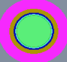
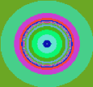
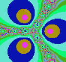
(A)	(B)	(C)

0.9 normal

Figure 3.5 : Attempts of improvements. The random palette coloring for attracting fixed points. More than the shading gradient approach, the attracting dynamics are evident here from the nested discs shrinking up to points.

One notices that this works finely with the neighboring dynamics, whose shrinking behavior to the attracting fixed point(s) is displayed step by step, or analogously in the neighborhood of a repelling point.

In the figures of tables 3.6 and 3.7, we painted all invariant sets (refer to fig. 2.3) which could possibly arise in the neighborhood of indifferent points $\delta$ by ordinary method, with emphasis to colors sequence and values accuracy.

The iterations of $f(z):z+z^{4}$ yield a ‘Fatou-Leau flower’ with $3$ petals meeting all together at the origin. Either with the aid of random palettes or as infinitesimal values of $\epsilon$ are set into inequality (3.1), one cannot evince the local dynamics, but only the basins shape. And no benefit is drawn from the experiments with irrationally indifferent points. In fig. 3.7/A and B, the random palette and a very high number of iterates were respectively tested to work with a Siegel disc case (it should appear in the green basin). The plot of an hedgehog was tested in (C, D). In particular, (B) and (D) use another coloring method which sets a one-to-one map between each point and the RGB cube, so that any complex point is univocally colored with regard to his location. Even if the iterative index $i$ increases to very huge values, orbits cannot reach too close to $\delta$ so we cannot get better pictures of it.

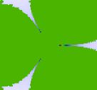
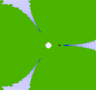
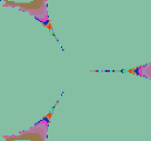
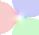
(A)	(B)	(C)	(D)

0.9 normal

Figure 3.6 : Ordinary attacks to rationally … . Different methods for the Fatou–Leau flower.

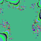
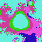
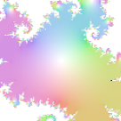
(A)	(B)	(C)	(D)

0.9 normal

Figure 3.7 : …and irrationally neutral points. Dynamics near a Siegel disc (A), (B) and an hedgehog (C), (D).

4 Off to ‘composite dynamics’

4.1 The core questions

What does to draw a local invariant set mean? And, in a larger sense, what do we want to get while drawing it?

Without basing upon good responses to these questions, it does not make so much sense to go on with our attempt. As remarked in table 2.2 at p. 2.2, holomorphic dynamics have different invariant sets.

Julia sets $J$ are easy to display: the only issues are merely technical (methods, palette colors, …). In local terms, the neighboring dynamics about points of $J$ can be easily collected under one easy concept: orbits, whose character is initially repelling near $J$, run across the basins $\mathcal{B}$ of attraction up to a (super–)attracting cycle (here, a fixed point $\delta$).

Some local invariant sets $\mathcal{I}_{s}$ around $\delta$ enjoy more or less complicated dynamics. The table 2.2 offered an overview of cases, where we noticed invariant sets endowed with ‘composite dynamics’, that is, involving more than one elementary motion: this is a bunch of information which is harder to be pulled out than when SFE commutes and there is only one local elementary motion to deal with. One should also take in account that the convergence speed of neighboring orbits may get slower as they reach closer to $\delta$: in this case, understanding such motions via colors is impracticable. Here one needs to evince either the (1) boundary $\partial\mathcal{I}_{s}$ (retrieving the ‘shape’) and the (2) inner motions (figuring out the ‘behavior’ of orbits).

Reaching (2) needs to consider that the elementary psychology of Space relates the perception of motion ‘to lines in the principal directions of curvature, which may communicate surface shape better than lines in other directions’ ([8], p. 43). This is a common feature of the field of Non-Photorealistic Rendering (NPR) and associated to the concept of ‘perceptually efficient images’, which is a visual representation emphasizing important features and minimizing superfluous details: our rendering are somehow skinny. For our context, we find useful to filter this concept by our needs: we want an analogously-shaped geometrical model of the given vector field, which is capable of evincing (1) and (2).

4.2 Obstructions (I) : no ticket for the ideal journey

The problem of drawing hedgehogs on a computer was first posed to the author by professor Pérez-Marco during an informal meeting in summer 2002. In general, the degeneration of a value $\theta\in{\mathbb{R}}\backslash{\mathbb{Q}}$ into $\theta\in{\mathbb{Q}}$ by finite digits machine computation is quite obvious.

Assuming the formula (2.6), one major issue is to check whether the resulting $\zeta=\theta^{n}$ may approximate irrationals poorly or not. One would like to distinguish the formal value $\theta$ with the input one $\alpha$ in practice, where $\alpha\approx\theta$ necessarily holds: here $|\alpha-\theta|=\varepsilon>0$. Analogously, one has $|\alpha^{n}-\theta^{n}|=\rho>\varepsilon>0$ for iterates, thus the error magnitude grows with the iterative index $n$. Resuming, we are not contented by the value $\theta$: how could we reduce $\rho$, if possible? In fact subtle issues may come up about the possibility: first, Cremer’s partition of irrational numbers shows that values of the null-measure set $\mathcal{N}$ are almost impossible to pick up by a machine with arbitrary precision, in order to guarantee the chosen invariant set: for example, hedgehogs $\mathcal{H}$ with no linearization area relate to extremely weak numerical conditions under the decimals cut-off, so that one could never watch them by relying on numerical computations. So would it make sense to approximate a number $\alpha^{n}\in{\mathbb{R}}\backslash{\mathbb{Q}}$ via another irrational $\theta^{n}$ which possibly enjoys different numerical properties? We reply that the value $\alpha^{n}$ may give rise to a local invariant set differing, more or less evidently, from what we really wanted from $\theta^{n}$. We observe that from Lebesgue null-measurability, it does not follows that $\mathcal{N}$ should be pointwise and totally disconnected; rather it consists of disjoint intervals whose amplitude is positive but infinitesimal, say, of width $\varepsilon$. If machine approximation may actually work under such interval $\varepsilon$, we might think of being able to get very good approximation of the original value $\alpha^{n}$ and of finding the related invariant set with adequate precision.

Without this chance, the approximation problem is weakly attainable on a numerical basis; is there an alternative attack relying on the approximation of properties? We recall that approximation in itself refers to another entity $\beta$, inexact and imitating (not copying) the original $\alpha$; so, dealing with properties, we questioned on whether it is plausible to seek one property relating to a third value $\beta$ and so that —α- β—¡—α- θ— holds? We would enter an ad infinitum process generating an infinitely many values $\xi,\gamma,\dots,\tau,$ and so that —α- β—¡—α- ξ—¡—α- γ—¡…¡—α- τ—¡—α- θ— and therefore infinitely many properties $\mathcal{P}$ standing between the formal value $\alpha^{n}$ and the practical value $\theta^{n}$ and even nested as follows: P_β⊂P_ξ⊂P_γ⊂ … ⊂P_τ⊂P_θ .

Question 4.1

Is the number of numerical properties finite? If so, how many they are?

We conjecture that the set of properties $\mathcal{P}$, involved in the local linearization around an irrationally indifferent $\delta$, is finite: because the topological configurations of hedgehogs are also finite.

4.3 Obstructions (II): practice is what matters

Now with regard to the practical computations involved in the iteration process, we can find three classes of obstructions:

1. Statistical: due to the $\mathcal{M},\mathcal{N}$ sets distribution over the real interval $[0,1]$, it much easier to pick up a $\theta\in\mathcal{M}$ than one $\zeta\in\mathcal{N}$. And due to above approximation, this task gets harder than ever.

2. Numerical: numbers $\theta\in\mathcal{M}$ are more robust to such approximation attack than $\zeta\in\mathcal{N}$; in fact, under iterates, Liouville numbers $\zeta$ tend to be turned into new values which are Diophantine irrationals; new resulting values cannot goodly approximate rational numbers and then one falls back into the Siegel disc case.

3. Procedural: Liouville’s condition is fundamental to plot hedgehogs, but it is also weak to be preserved under iteration. The movement rate or orbits in the hedgehog $\mathcal{H}$ gets as slower as closer to the fixed $\delta$. Thus one would be pushed to increase the iteration index $n$ to get finer results but we saw the iteration process supports obstructions 1 and 2.

Approximation and computer usage are two ‘obstructions’ we cannot overcome. Not having a valid solution at hand nor being successful to find it, the problem was left open until we occasionally came to it during March 2006, when we planned to find a strategy for lessening the break of irrationality. It was clear that the numerical path was impracticable.

Our problem with hedgehogs refers back to the impossibility of drawing local invariant sets, where slower and slower convergence rates, as iterates are closer to $\delta$, escape the possibilities offered by the standard methods: in the next section, an analysis on the ordinary graphical methods for holomorphic dynamics will be given in order to motivate their exclusion from the run for displaying local invariant sets and, most important, hedgehogs accurately.

4.4 Quality vs. quantity

The methods described in section 3 are structurally weak for our purposes: the reader shall know that they have been developed (read, customized) for iterates of polynomial maps, in primis the quadratic $f(z):z^{2}+c$, where $z,c\in{\mathbb{C}}$ and $c$ is a parameter. As we showed here and even for quaternionic Julia sets, as discussed by the author in [16, 17], they might not work finely or even they may fail completely if exported to dynamical systems which are distinct from their original context. We remark that, mostly due to the very slow convergence rate of orbits near the indifferent $\delta$, the escape time approach is inconvenient to display the hedgehogs, either if different colors sets are applied or if the index $i$ is hugely increased. Ordinary methods work quantitatively and they fail with dynamics wanting the sharpest numerical precision; in addition, the geometry of these invariant sets (both in local and global terms) is exclusively retrieved by the value of the last iterated point $z_{m}$, where $m$ is any largest iterative index $i$ available to the machine architecture. We may set $m$ to the largest value then, but computations would be excessively time consuming.

In the spirit of automatism helping to save time, we state that a radically different method is required: thus a way out is not to reach to those neighborhoods, but to ‘be-already-there-and-work’. Even in this new direction, the method customization is required: in fact, we judged useful to adopt an half-way strategy which, besides the inevitable finite digits computation, teams up with a qualitative attack by the imitation of a model with pre-defined shape.

The decision on the model matured after the conclusions in section 2.2, where the failure of SFE for Fatou-Leau flowers and hedgehogs implied that such dynamics cannot be adequately described by models based upon regular curves, such as concentric circles or sheaves of straight-lines. So we wanted to adopt a non–regular and, mostly, topologically equivalent model. Namely, this is the (holed) $n^{th}$-branched star, as depicted in table 5.11. It is extremely important to remark that the following results are based upon the iteration of quadratic germ (2.5). Actually there exist obstructions of theoretical nature, stopping to extend the results from quadratic holomorphic germs to higher degrees.

5 Re-elaborating the equi-potentials

5.1 The holed $n$-th branched star model

Our approach roots to nothing new in digital graphics for dynamical systems and often used in complex analysis. Known under the term of ‘equi-potential curves’, the reader can find examples of it in [12] by Needham and, for holomorphic dynamics, in [11] by Milnor – although it already appeared, but weakly, in older publications [13, 15]. The further pseudo–code, reported to support the concept rather than being implemented as it is, consists of a main routine assuming the whole input finite subregion of ${\mathbb{C}}$ as a grid of seeds $z$ and filtering the dynamics of each iterated point $z_{n}$ via a sub-routine checking if an orbit can be possibly plot, according to the holed star model.

    #include "complex.h"  // this is a class handling complex numbers
                          // downloadable from author’s site

    complex fxd_pt ;      // we assume that we already
    fxd_pt.real = 0.0;    // know the location of the fixed point
    fxd_pt.imag = 0.0 ;   // around which we want to plot the hedgehog

    double val = 0, tmp_val = 0 ;   // values which will be later
                                    // stored and compared
    BOOL bInitFlag = FALSE ;        // this boolean flag will be
                                    // to check the two above [double] values

    // we assume that the four coordinates of the screen port where
    // the image will appear are stored in these variables;

    int top = 0, bottom = 320, left = 0, right = 200 ;
    complex z ;

    for ( x = left + 1; x < right ; x++ )
    {
        for ( y = top + 1; y < bottom ; y++ )
        {
            // suggestion: do a converse estimation map to come from screen
            // coordinates to the complex point z further by ’RescaleToMap’
            // so that you’re assured that decimals approximation
            // does not make more than one screen point to the same
            // complex point z

            rescale-the-pair ( x, y ) to-the-pair ( z.real, z.imag );
            ////////////////////////////////////////////////////////////

            // at this point you shall just iterate the function
            // for the required number of steps but without
            // test conditions. See previous code.
            // Just stop it by a iterative top index limiter.

            // We did not show any related code for the function
            // to be iterated because one needs more complicate
            // explanations.
            // Make sure you are working with a suitable function
            // retrieving an hedgehog. We suggest you to use the one
            // an holomorphic quadratic and indifferent germ where
            // the angle theta is represented by the continuous fraction
            // reported further.

            // We can say we coded a complex parser
            // to input any function even in the form; sorry
            // but the latex syntax is the best we can use to
            // arrange one example:
            // f(z) : e^(2\pi i\theta)z+z^2

            complex output_z = iterate-the-function f(z) ;

            // NOTE : if you input the identity map, you’ll see
            // the holed branched star.

            BOOL bDraw = Holed_Star( output_z, fxd_pt, double& val,
                                     double& tmp_val, BOOL& bInitFlag ) ;

            if ( bInitFlag )
            {
                if ( val != tmp_val )
                {
                    if ( bDraw ) pDC->SetPixel( x, y, 0 );
                    val = tmp_val ;
                }
            }
            else bInitFlag = TRUE ;
        }
    }

In the previous code, one sees a raster scan of the screen by rows (y) and columns (x). As integer coordinates are taken per each screen point, they have been immediately turned into real and imaginary values respectively, so to have finally the complex point z.

And now we give the code details for the function Holed_Star which draws the hedgehogs/holed star by equi-potentials point after point. In this code, we just presented monochromatic hedgehog (refer to table 5.11, A/B), the colored version requires one more function which we chose to not include here for code simplicity.

BOOL Holed_Star( complex z, complex fxd_pt, double& val,
                 double& tmp_val, BOOL& bInitFlag )

{
    #include "complex.h" // this is a class handling complex numbers
                         // downloadable from author’s site

    #define PI 3.14159265358979323846  // we need PI to be as
                                       // precise as possible

    complex tmp_z = z ;         // we need another variable for
                                // storing a temporary value later

    double branches_number = 12 ;      // this explains itself !
    double offset = 0.5 ;              // this is the radius of the
                                       // disc hole in the star
                                       // if set to zero, the disc is empty

    double existence_interval = 2.0 * PI ;   // the values range in which
                                             // compute all branches location
                                             // in radial terms

    double potential_rate = existence_interval / branches_number ;

    tmp_z -= fxd_pt ;            // performs a translation of all points
                                 // so that the fixed point maps to the
                                 // origin and the further computations
                                 // get easier
    double v = tmp_z.angle();

    double out_level = ( f.euclidean_dist( z ) <= offset ) ? -1 : v / potential_rate ;

    int ol = (int)out_level ;       // we need an integer value for the
                                    // output level to be eventually used
                                    // for color the point

    if ( !bInitFlag ) val = ol ;    // if the flag was not set,
                                    // then this means that it is the first ever
                                    // value to be stored.
    else tmp_val = ol ;             // Otherwise, it does not. See before
                                    // in the main function

    if( ol < 0 || ol > branches_number )     // check for values not
                return FALSE ;               // ranging out of the interval

    return TRUE ;
}

We have now a bunch of code to scan a region $\mathcal{R}\subset{\mathbb{C}}$, so that Holed_Star classifies the $n$–fold image region $f_{n}(\mathcal{R})$ via the star model.

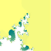
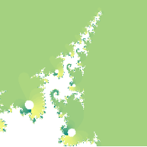
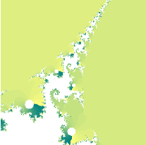
(A)	(B)	(C)

0.9normal

Figure 5.8 : Wedging the bounded basin (II). Three close-ups of the Julia set $J$ for the function (2.5) with $\theta$ expressed by (5.1), rendered by the holed star model. The iteration index was set at (A) 150, (B) 300 and (C) 1000 respectively. White disks are preimages of the hole in the star, while colours are changing due to iteration values attained by the forward images at different ranks. The wedging action of the hedgehogs generation is evident.

5.2 Unveiling the code

Here we explain the elaborations worked by part of the code in section 5.1. First one shall focus on this line:

double out_level = ( f.euclidean_dist( z ) <= offset ) ? -1 : v/potential_rate ;

if the point z, resulting from the iteration process, is farther from the fixed point f than a preset distance offset, the ratio v/potential_rate shall be computed to know whether one paints that iterated point black or not; otherwise, the negative value $-1$ will be used as a flag, indicating that the point must not be tested for further painting. The variable offset stores the radius value for the hole in the star model.

The value v is the angle of the last image z in the current orbit and helping to have that point location in relation to the branches. One also notices that

 double potential_rate = existence_interval / branches_number ;

which, applied to the first line of code, let v / potential_rate turn into index=v⋅branches_numberexistence_interval=vexistence_interval⋅branches_number the ratio factor in the right member is normalized in the unit interval [0,1]; when multiplied by branches_number, one finds that: 0 $\footnotesize<$ index $\footnotesize<$ branches_number, so it ranges inside the interval of arbitrary input number of branches. If decimal values are retrieved, they shall be rounded off to the integer part, because decimals do not make sense in terms of branches index. For example, given $31$ branches for an holed star, like in table 5.10, we expect that the index ranges in [0,30]. The product with the branches_number yields the branch index for the last computation of the $n$–iterated image z. It is reasonable that watching hedgehogs pictures one first wonders: given a white background, how come are black lines painted exclusively? And, in addition, since the black pixels refer to those only points to be painted, why are others not painted? One side implication from a general method based upon equi-potentials is that screen points are plot only if the current equipotential is trespassed.

In our computational model, the geometry locus of the curves is the qualitative part. This locus is often detected by a formula: for example $|z-\zeta|=R$ is known to detect a circle centered at $\zeta$ and if ‘$=$’ replaces with ‘$<$’, we deal with the open disc.

In order to meet machine requirements operativity, we shall deal with quality in terms of quantity: therefore, each curve matches one only index value. When we point out to a curve or to a branch in the star model, we want its index essentially. With ‘an equipotential level was trespassed’, we mean that the current index value has changed. For a set of points retrieving a same index, only the first one shall be plot; again, if the indexes of two consecutive points are different, the second point is plot. Algorithmically speaking, one stores the last index and, if it equals the previously stored value, no equipotential is was trespassed; otherwise, it was and one paints the related point black. So the implication is straight-forward: Different indexes→Different equipotential→Trespass→Paint the point.

For example, if we associate each screen point to its resulting index, we find a chain of indexes indicating how pixels and the entire screen row is regarded in this raster process from left to right: 1-1-1-2-2-2-2-2-2-3-3-3-3-4-4-4-4-2-2-2-5-5-5-5-3-3-3-3-3 The index in bold makes the difference and arrests the previous sub-sequence of same indexes: the related point will be painted black. Technically, this can be easily understood by handling the boolean flag bInitFlag of the main routine at section 5.1. The reader would take care that as the bInitFlag is set, the values for comparison were stored in the two variables val and tmp_val, as shown here in the following resume of the previous code:

BOOL bDraw = Holed_Star( output_z, fxd_pt, double& val, double&
tmp_val, BOOL& bInitFlag ) ;

if ( bInitFlag )
{
    if ( val != tmp_val )
    {
        if ( bDraw ) pDC->SetPixel( x, y , 0 );

        val = tmp_val ;
    }
}
else bInitFlag = TRUE ;

It is clear that the point is painted black (RGB value is $0$) only when

if ( val != tmp_val )

is satisfied. If so, the old equipotential was trespassed. We jumped into another equipotential level (iterations are a discrete model of a continuous map and jumps are solely achieved onto the successive or onto the preceding equipotential level). And we take the new value as the referring one by val = tmp_val ;

5.3 The pro(s) and con(s)

Benefits: the fate of orbits $f^{n}(z):z_{n}$, which finally land on a same equipotential level $\mathcal{R}$ – the bounded region radially distributed around $\delta$, is grouped by the seed points $z$ under the same color, according to our approach to ‘be-already-there-and-work’ (p. 4.4). From the early works by Cherry [6] and the latest production by Pérez-Marco [14], hedgehogs dynamics can be simply resumed as follows ([6], p. 33):

“…as it progressively deformed through starfish shapes […] consisting of an infinity or ‘rays’ emanating from $O$; each such ‘ray’ is a connected closed set, and ‘most’ of them are arbitrarily short. A $z_{0}$ on any of these rays gives a chain ($z_{n}$) each of whose points lies on another of them …”

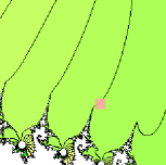
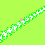
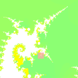
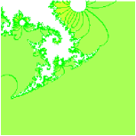
(A)	(B)	(C)	(D)

0.9normal

Figure 5.9 : Wedging the bounded basin (III) By zooming in the red square region in succession, we follow the wedging action of the hedgehog inside the basin boundary. (A) without requiring a huge number of iterates (just 100 here) the contour is able to show how the hedgehog makes its way into the basin. (B–D) There are several smaller and smaller fjords emanating from the longest arm which runs towards the linearization domain (whether it is empty or not).

Hence the hedgehog boundary $\mathcal{H}$ of the regions $\mathcal{R}$ wedges the bounded basin, which gets thinner and thinner as the iterative index $n\rightarrow\infty$. The final shades distribution helps to evince the topology of $\mathcal{H}$ (figs. 5.8), but a major benefit comes from the contour plot of all such $\mathcal{R}$ ; contours allow to watch the complete hedgehog topology, by a comparatively little iterative index, while other methods, even if pushed to the top machine performance, would have not reached so far.

Good pictures on the way $\mathcal{H}$ wedges the bounded basin are granted because of the holed star fits the hedgehogs topology, without needing to input very huge indexes for having almost the same results which previous standard methods: in fact they suffer the very slow accumulation rate of neighboring orbits $z_{n}$ about $\delta$. This achievement completely fills the lack of the approaches discussed before.

Lacks: more than any other equipotential model, the holed star does not grant an ‘intelligent approach’, that is, capable of fitting any input function $f(z)$ as best. Equi-potential curves are just as a sort of elastic sheet being stretched by $f(z)$: they are used to watch the local dynamics via lines distribution, but an a priori knowledge about the property of given dynamics is required to choose the best model to depict them, among a bunch featuring a given equi-potential curves distribution (horizontal or vertical straight-lines, concentric discs, stars), each one working differently on the current case, thus being restrictedly indicative on the function behavior. Hence we may look at equi-potential models are differently styled interpreters and, like for any interpretative process, one must speak the same ‘language’ adopted, here of the dynamics of $f(z)$, for best understanding: so the essence of any model is to play as both the proper syntax and as the fittest dictionary to achieve the correct ‘translation’. Hedgehogs and holed star model do not escape this rule, so that the fine tunings can secure the most adherent results. This is not so difficult however, anyway the star model is less ‘ready-to-go’ than concentric circles or straight lines distributions of equi-potentials, because of one more parameter to tune, namely the hole radius, in order to properly plot the variety of hedgehogs, as listed at p. 2.3.

5.4 Tuning the disc radius

Being this one an empiric approach, one needs to tune some parameters to ‘grasp’ the finest pictures of hedgehogs, letting their characters to match with the real figure as closer as possible. In figures at table 5.10, one tunes the maximal disc/hole radius $r_{\mathcal{S}}$ for which the hole of our branched star model would look like a disc: the response from too large values (fig. 5.10/A) offers a strongly deformed curve indeed, while smaller ones may not evince the effective extension of the Siegel compactum. Thus one has to try to decrease the radius value $r_{\mathcal{S}}$ until the disc comes out.

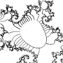
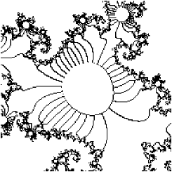
(A) $r_{\mathcal{S}}=0.20$		(B) $r_{\mathcal{S}}=0.15$
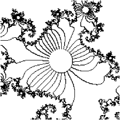
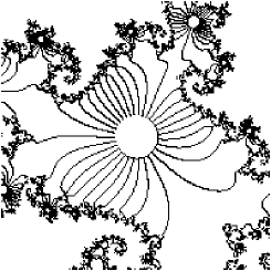
(C) $r_{\mathcal{S}}=0.10$		(D) $r_{\mathcal{S}}=0.09$

Figure 5.10 : The radius test. Tuning the radius $r_{\mathcal{S}}$ of Siegel compactum.

The author is working on a theory to retrieve sharp estimation of such radius metric, as well as for the Siegel disc [18]: this might be helpful to finally have very fine pictures of hedgehogs.

5.5 Stars and equivalent classes

As shown, orbits accumulate at their forward invariant limit sets. In the case of hedgehogs, whether the linearization disc is small or has zero area, the holed $k$-th branched star is a model describing this accumulation in the same way as neighboring orbits do. The star model benefits are two-fold: while the regions imitate as best as possible such dynamics inside the bounded basin, the branch lines are screening the shape of the basin $\mathcal{B}_{\infty}$ to $\infty$. Since the latter and the bounded basin are complementary sets, in terms of converging orbits, tracking down their shapes equals to know the hedgehog topology.

With regard to the star and the regions between, orbits are parted into equivalence classes E_1,E_2,…,E_k, where $k$ is the number of the branches. The basin $\mathcal{B}_{\infty}$ to $\infty$ does not belong to any class $\mathcal{E}$, thus it does not belong to $\displaystyle\bigcup_{n=1}^{k}\mathcal{E}_{n},$ since the union is the bounded basin $\mathcal{B}_{\delta}$ itself. In the holed star model, $\mathcal{B}_{\delta}$ is mapped to the union of the regions between the branches.

The branches of the star model elongate from the outer region up to the disc, or to the center point if the hole has zero area: this is not merely obvious and plays relevantly during orbits classification. In fact, in a similar fashion but applied to iterates, the imitation of the branches distribution allows to track down the wedging action of $\mathcal{B}_{\infty}$ up the boundary of the hole or, again, to the center of the star when the hole is empty: even here, consequentially, the wedging action by $\mathcal{B}_{\infty}$ to $\mathcal{B}_{\delta}$ helps to deduce the hedgehog shape (This is the reason why one should already know the possible existence of the hole, i.e. of a linearization area with positive radius.) As remarked differently in section 5.3, one great benefit is the imitation up to the hole boundary. In fact, nearly iterates get slower and slower to converge or even their might not converge at all for hedgehogs. The imitation of branches distribution allows to break down the slow convergence barrier and the resulting line show the orbits fate, even after a relatively slow number of iterates (see figs. 5.9).

In fact the equivalence classes allow to reconstruct the basins distribution in the same fashion of the star model: so one also understands why it also works finely with the Fatou-Leau flower, a similarly shaped vector field, where one basin wedges the other.

5.6 Displaying the Fatou-Leau flowers

The holed star immediately worked very finely with topologically equivalent invariant sets, so one might like to consider the benefits from this new graphical construction and focus on the Fatou-Leau flowers in table 5.12 before moving definitely to hedgehogs.

Definition 5.1

Fatou-Leau flower. If $\hat{z}$ is a fixed point of multiplicity $n+1\geq 2$, then there exist attracting petals $\mathcal{P}_{1},\mathcal{P}_{2},\dots,\mathcal{P}_{n}$ for the $n$ attracting directions at $\hat{z}$, a repelling petals $\mathcal{P}^{\prime}_{1},\mathcal{P}^{\prime}_{2},\dots,\mathcal{P}^{\prime}_{n}$ for the $n$ repelling directions, so that the union of these $2n$ petals, together with $\hat{z}$ itself, forms a neighborhood $N_{0}$ of $\hat{z}$. ([11], p. 105)

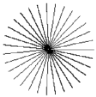
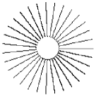
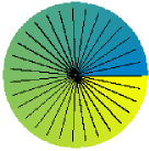
(A)	(B)	(C)	(D)

0.9 normal

Figure 5.11 : I am the star. The (holed) $n^{th}$-branched star in monochromatic and colored versions.

One first notices that straight lines meet at the origin and they lie at the attracting directions, whereas the divergent ones are deformed into petals shaped curves.

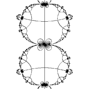
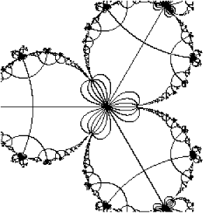
$z+z^{3}$		$z+z^{4}$
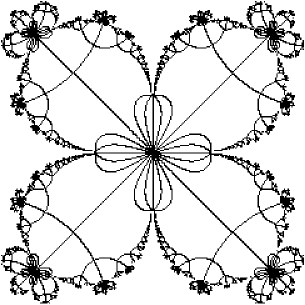
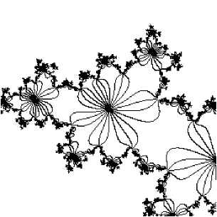
$z+z^{5}$		$e^{2\pi it}z+z^{2},\quad t=3/7$

0.9 normal

Figure 5.12 : A bunch of flowers to the star. The application of the holed star to different cases of Fatou-Leau’s flowers.

It is useful to remark that straight lines leading to the origin are adjacent to converging orbits: the imposition of the holed star model lessens the difficulty of reaching closer neighborhoods of $\delta$, owing to the slow convergence rate inside. Thus the computation and display of such flowered invariant set may be a good entry point for realizing the benefits of such a qualitative approach and the need of tuning properly the parameters of the star, such as the radius hole (set to $0$ for flowers) and the branches number, especially for hedgehogs.

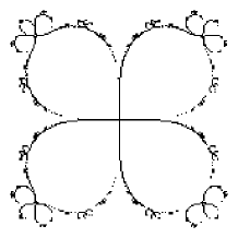
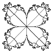
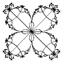
(A)		(B)		(C)
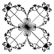
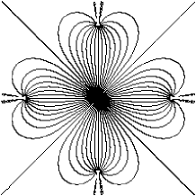
(D)		(E)

0.9 normal

Table 5.3 : Tuning the number of branches. We chose for this example the function $f(z):z+z^{5}$, which yields a flower with $4$ petals. The best performance for the holed branched star is to have some branches adjacent to both the $4$ converging and the $4$ attracting directions; then it is wise to set the branches number to multiples of $4$. The other branches are useful to understand the dynamics. Without them we should just see straight lines, as depicted in (A). So we have 4, 8, 16, 32 and 64 branches for figures (A), (B), (C), (D), (E) respectively.

5.7 Experiments with hedgehogs

This latter aspect should be greatly taken into account for hedgehogs too.

[11] (p. 123) was rather inspiring to try enhancing their graphics by focusing on an imitation graphical model based upon equi-potentials; this book also includes one formula and one figure of a quadratic holomorphic germ providing an hedgehog. Here the irrational angle $\theta$ can be expressed in terms of the continuous fraction expansion

$$\frac{1}{3+\frac{1}{10+\frac{1}{20000+\dots}}}.$$ (5.1)

The choice of such model was not at random: the different approaches in table 5.13 lack of displaying the true shape, so that at last the holed star was chosen to best imitate the general hedgehog shape under iteration, when the Siegel compactum is empty or even arbitrarily small. At this concern, setting the right number of branches improves the figure.

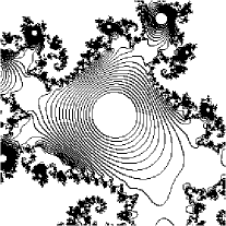
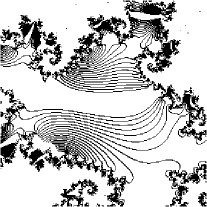
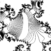
(A)	(B)	(C)

0.9 normal

Figure 5.13 : Different equi-potential models. The failures to evince the hedgehog shape: concentric disks, vertical and horizontal lines distributions are displayed in figures (A), (B) and (C) respectively. Finest figures need the most equivalent equi-potential model.

Our approach wants to exploit the equi-potentials method by looking at the deformation of the (holed) $n^{th}$-branched star. One notices the existence of curves indicating the wedging action into wedging $\mathcal{B}_{\delta}$; this was not evident from figures 3.7/C and D by ordinary methods. Although we cannot depict a detailed shape of fjords, we may at least understand where they will get to.

As we showed, this is not an intelligent method. Thus finest drawings require to already know the hedgehogs features, like the the radius of the Siegel compactum and number of fjords, regions where $\mathcal{B}_{\infty}$ penetrates $\mathcal{B}_{\delta}$) and modelled by the star branches.

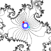
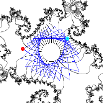
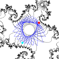
(A)	(B)	(C)

0.9 normal

Figure 5.14 : Neighboring dynamics. Figure (A) shows the rotatory motion of iterates in the Siegel compactum, while outer orbits are shown in (B) and (C).

6 Conclusions

In author’s opinion, well-drawn figures of local invariant sets necessarily want customized approaches: equi-potential approach is looking like the best performing today and is could be even optimized when topologically equivalent model are applied; thus a general method to be applied for displaying a given local invariant set, independent on the input map, seems a utopia. But, being open to the possibilities offered by Science, one optimistically says ‘up to now !’

Alessandro Rosa

zandor_zz@yahoo.it

References

- [1] Alexander D.S., Iavernaro F., Rosa A., Early Days in complex dynamics, in preparation.
- [2] Beardon A.F., Iteration of rational functions, Springer & Verlag, 1991.
- [3] Binder I., Braverman M., Yampolsky M., On computational complexity of Siegel Julia sets, Commun. Math. Phys, preprint.
- [4] Buff X., Chéritat A., On the size of quadratic Siegel disks. Part I, Prepublication du Laboratoire E. Picard, n. 267, Toulouse, France, 2003.
- [5] Buff X., Chéritat A., Upper bound for the size of quadratic Siegel disks, Inventiones Mathematicae, 156, 1, 2004, pp. 1–24.
- [6] Cherry T.M., A singular case of iteration of analytic functions: a contribution to the small divisors problem, Non-linear problems of Engineering, Academic Press, New York, 1964, pp. 29-50.
- [7] Cremer H., Zum Zentrumproblem, Math. Annalen, 98, 1927, pp. 151-163.
- [8] Girshick A., Interrante V., Haker S., Lemoine T., Line direction matters: an argument for the use of principal directions in 3D line drawings, Non-Photorealistic Animation and Rendering, Proceedings of the 1st international symposium on Non-photorealistic animation and rendering, Annecy, France, 2000, pp. 43–52.
- [9] Liverani C., Turchetti G., Improved KAM estimates for the Siegel radius, Journal of Statistical Physics, Volume 45, Numbers 5-6, 1986, pp. 1071–1086.
- [10] Markosian L., Kowalski M.A., Trychin S.J., Bourdev L.D., Goldstein D., Hughes J.F., Real-Time Nonphotorealistic Rendering.
- [11] Milnor J.W., Dynamics in one complex variable, 2 edition, Vieweg, 2000.
- [12] Needham T., Visual complex analysis, Oxford Press, 2000.
- [13] Peitgen H.-O., Jürgens H., Saupe D., Chaos and Fractals, Springer & Verlag, 1991.
- [14] Pérez-Marco R., Fixed points and circle maps, Acta Mathematics, 179, 1997.
- [15] The Science of Fractal Images, edited by Heinz-Otto Peitgen and Dietmar Saupe, Springer-Verlag, New York, 1988.
- [16] Rosa A., Methods and applications to display quaternion Julia sets, Electronic Journal of Differential Equations and Control Processes, St. Petersburg, 4, 2005.
- [17] Rosa A., On a solution to display non-filled-in quaternionic Julia sets, arXiv cs.GR/0608003.
- [18] Rosa A., The accessibility locus theory and its applications to iterates of functions in one complex variable, in preparation.
- [19] Yoccoz J.C., Linéarisation des germes de difféomorphismes holomorphes de , Comptes Rendus Acad. Sci. Paris, Sér. I Math 306, 1988, pp. 55–58.
- [20] Yoccoz J.C., Recent developments in dynamics, Proceedings of the International Congress of the Mathematicians in Zürich, Birkhäuser Verlag, 1994.