Throughput Optimal Distributed Control of Stochastic Wireless Networks

Abstract

The Maximum Differential Backlog (MDB) control policy of Tassiulas and Ephremides has been shown to adaptively maximize the stable throughput of multi-hop wireless networks with random traffic arrivals and queueing. The practical implementation of the MDB policy in wireless networks with mutually interfering links, however, requires the development of distributed optimization algorithms. Within the context of CDMA-based multi-hop wireless networks, we develop a set of node-based scaled gradient projection power control algorithms which solves the MDB optimization problem in a distributed manner using low communication overhead. As these algorithms require time to converge to a neighborhood of the optimum, the optimal rates determined by the MDB policy can only be found iteratively over time. For this, we show that the iterative MDB policy with convergence time remains throughput optimal.

I Introduction

The optimal control of multi-hop wireless networks is a major research and design challenge due, in part, to the interference between nodes, the time-varying nature of the communication channels, the energy limitation of mobile nodes, and the lack of centralized coordination. This problem is further complicated by the fact that data traffic in wireless networks often arrive at random instants into network buffers. Although a complete solution to the optimal control problem is still elusive, a major advance is made in the seminal work of Tassiulas and Ephremides [1]. In this work, the authors consider a stochastic multi-hop wireless network with random traffic arrivals and queueing, where the activation of links satisfies specified constraints reflecting, for instance, channel interference. For this network, the authors characterize the stability region, i.e. the set of all end-to-end demands that the network can support. Moreover, they obtain a throughput optimal routing and link activation policy which stabilizes the network whenever the arrival rates are in the interior of the stability region, without a priori knowledge of arrival statistics. The throughput optimal policy operates on the Maximum Differential Backlog (MDB) principle, which essentially seeks to achieve load-balancing in the network. The MDB policy (sometimes called the “backpressure algorithm”) has been extended to multi-hop networks with general capacity constraints in [2] and has been combined with congestion control mechanisms in [3, 4].

While the MDB policy represents a remarkable achievement, there remains a significant difficulty in applying the policy to wireless networks. The mutual interference between wireless links imply that the evaluation of the MDB policy involves a centralized network optimization. This, however, is highly undesirable in wireless networks with limited transmission range and scarce battery resources. The call for distributed scheduling algorithms with guaranteed throughput gives rise to two main lines of research.

One approach is to adopt simple physical and MAC layer models and apply computationally efficient scheduling rules in a distributed manner. The work in [5, 6] study networks where at any instant only mutually non-interfering links are activated, and any link, as long as it is active, transmits at a fixed rate. In particular, it is shown in [5] that Maximal Greedy Scheduling can achieve a guaranteed fraction of the maximum throughput region. This result is generalized in [6] to multi-hop networks where the end-to-end paths are given and fixed. Despite its simplicity, the distributed scheduling considered in the above work applies to only a limited class of networks. Moreover, the simplicity is gained at the expense of throughput optimality [7].

Another line of research develops distributed power control and rate allocation algorithms for implementing the MDB policy with the aim of preserving the throughput optimality. Thus far, distributed MDB control has been investigated only for networks with relatively simple physical layer models. For example, Neely [8] studies a cell partitioned network model where different cells do not interference with each other so that scheduling can be decentralized to each cell. However, the question of how the MDB policy can be efficiently applied in general wireless networks remains unanswered.

In this paper, we consider the implementation of the MDB algorithm within interference-limited CDMA wireless networks, where transmission on any given link potentially contends with interference from all other active links. In this setting, we present two main sets of results. First, we develop a set of node-based scaled gradient projection power control algorithms which solves the MDB optimization in a distributed manner using low communication overhead. As these algorithms require time to converge to a neighborhood of the optimum, the optimal rate allocation of the MDB policy can only be found iteratively over time. In the second result, we show that the iterative MDB policy with convergence time remains throughput optimal as long as the second moments of the traffic arrival rates are bounded. Combining these two results, we conclude that our algorithms yield a distributed solution to throughput optimal control of CDMA wireless networks with random traffic arrivals. The framework and techniques developed in this work can readily be adapted to general interference-limited stochastic wireless networks.

Iterative implementation of the MDB policy has also been studied independently by Giannoulis et al. [9]. They investigate distributed power control algorithms for CDMA networks which are iterated once for every update of the queue state. In their scheme, the power and rate allocation algorithms are iterated only once in a slot, after which the queue state is re-sampled. In contrast, our algorithms re-sample the queue state only after the power and rate allocation has converged to the optimum for the previous queue state. We provide a rigorous proof for the throughput optimality of our scheme using a novel geometric method. We also compare the performance of our scheme with that of the non-convergent iterative algorithms in [9] and of the centralized MDB policy (whereby it is assumed that the optimal powers and rates are instantaneously obtained given the queue state) through simulations. In the experiments we conducted, the iterative MDB policy with convergence outperforms that without convergence.

This paper is organized as follows. Section II introduces the model of stochastic multi-hop wireless networks and reviews the throughput optimal Maximum Differential Backlog policy. The node-based power control algorithms that achieve the optimal rate allocation are presented in Section III. In Section IV, we prove that the iterative MDB policy proposed in the last section maintains the throughput optimality even in the presence of non-negligible convergence time. The comparison of different implementations of the MDB policy is conducted through simulations in Section V.

II Network Model and
Throughput Optimal Control

II-A Model of Stochastic Multi-hop Wireless Networks

Consider a wireless network represented by a directed and connected graph $\mathcal{G}=({\cal N},{\cal E})$. Each node $i\in{\cal N}$ models a wireless transceiver. An edge $(i,j)\in{\cal E}$ represents a unidirectional radio channel from node $i$ to $j$. For convenience, let ${\cal O}(i)\triangleq\{j:(i,j)\in{\cal E}\}$ and ${\cal I}(i)\triangleq\{j:(j,i)\in{\cal E}\}$ denote the sets of node $i$’s next-hop and previous-hop neighbors, respectively. Let the vector $\boldsymbol{h}=(h_{ij})_{(i,j)\in{\cal E}}$ represent the (constant) channel gains on all links.

Denote the transmission power used on link $(i,j)$ at (continuous) time $\tau$ by $P_{ij}(\tau)\geq 0$, and the instantaneous service rate of link $(i,j)$ by $R_{ij}(\tau)\geq 0$. A feasible service rate vector $\boldsymbol{R}(\tau)=(R_{ij}(\tau))_{(i,j)\in{\cal E}}$ must belong to a given instantaneous feasible rate region ${\cal C}(\boldsymbol{P}(\tau))$ reflecting the physical-layer coding mechanism. Under peak power constraints $\hat{P}_{i},i\in{\cal N}$, let

$$\Pi=\left\{\boldsymbol{P}(\tau)\in\mathbb{R}_{+}^{|{\cal E}|}:~{}\sum_{j\in{\cal O}(i)}P_{ij}(\tau)\leq\hat{P}_{i},\forall i\in{\cal N}\right\}$$

be the set of feasible power allocations and

$${\cal C}(\Pi)\triangleq{\rm conv}\left(\bigcup_{\boldsymbol{P}\in\Pi}{\cal C}(\boldsymbol{P})\right)$$

be the long-term feasible service rate region. Here, the convex hull operation ${\rm conv}(\cdot)$ indicates the possibility of time sharing among different feasible power allocations $\boldsymbol{P}\in\Pi$ over a sufficiently long period.

Let the data traffic in the network be classified according to their destinations. Traffic of type $k\in{\cal K}$ is destined for a set of nodes ${\cal N}_{k}\subset{\cal N}$ (when type $k$ traffic reaches any node in ${\cal N}_{k}$, it exits the network), where ${\cal K}$ is the set of all traffic types. Let $T>0$ be a given time slot length. Let the number of bits of type $k$ entering the network at node $i$ from time $tT$ to $(t+1)T$ be a nonnegative random variable $B_{i}^{k}[t]$. Assume that for all $t\in\mathbb{Z}_{+}$, $B_{i}^{k}[t]$ are independent and identically distributed with $\mathbb{P}(B_{i}^{k}[t]=0)>0$. Let $\mathbb{E}B_{i}^{k}[t]=a_{i}^{k}<\infty$ and $\mathbb{E}\left(B_{i}^{k}[t]\right)^{2}=b_{i}^{k}<\infty$ be the first and second moments of $B_{i}^{k}[t]$. Furthermore, assume all arrival processes $\{B_{i}^{k}[t]\}_{t=1}^{\infty}$, $i\in{\cal N},k\in{\cal K}$ are mutually independent.

Assume node $i\in{\cal N}$ provides a (separate) infinite buffer $i^{k}$ for each type $k$ of traffic that is not destined for $i$. Denote the unfinished work in $i^{k}$ at time $\tau$ by $U_{i}^{k}(\tau)$. We focus on the queue states sampled at slot boundaries $\tau=tT$, $t\in\mathbb{Z}_{+}$. Let $U_{i}^{k}[t]$ denote the instantaneous backlog at the beginning of the $t$th slot, i.e., $U_{i}^{k}[t]=U_{i}^{k}(tT)$. Over the $t$th slot, link $(i,j)$ serves $i^{k}$ at rate $R_{ij}^{k}[t]=\int_{tT}^{(t+1)T}R_{ij}^{k}(\tau)d\tau$. The aggregate service rate on link $(i,j)$ over the $t$th slot is $R_{ij}[t]=\sum_{k\in{\cal K}}R_{ij}^{k}[t]$. Thus, we have the following queueing dynamics:

$$\begin{array}[]{l}U_{i}^{k}[t+1]\leq\\ \left(U_{i}^{k}[t]-\displaystyle\sum_{j\in{\cal O}(i)}R_{ij}^{k}[t]+\displaystyle\sum_{m\in{\cal I}(i)}R_{mi}^{k}[t]+B_{i}^{k}[t]\right)^{+}.\end{array}$$ (1)

Here $(x)^{+}$ denotes $\max\{x,0\}$, and the inequality comes from the fact that in general, since certain queues may be empty, the actual endogenous arrival rate is less than or equal to the nominal rate $\sum_{m\in{\cal I}(i)}R_{mi}^{k}[t]$.

II-B Stability Region and Throughput Optimal Policy

Given the wireless network model, we now define notions of stability and investigate throughput optimal control policies.

Definition 1

[2] The queue $i^{k}$ is stable if $g_{i}^{k}(\xi)\triangleq\lim\sup_{n\rightarrow\infty}\frac{1}{n}\sum_{t=1}^{n}\mathbb{P}\left[U_{i}^{k}[t]>\xi\right]\rightarrow 0$ as $\xi\rightarrow\infty$. Input processes $\{\boldsymbol{B}[t]=(\boldsymbol{B}_{i}^{k}[t])_{i\in{\cal N},k\in{\cal K}}\}_{t=1}^{\infty}$ are stabilizable if there exist service processes $\{R_{ij}^{k}[t]\}$ for all $(i,j)\in{\cal E}$ and $k\in{\cal K}$ such that for every $t\in\mathbb{Z}_{+}$, $\boldsymbol{R}[t]\in{\cal C}(\Pi)$, and the resulting queueing processes are all stable.

Definition 2

The stability region $\Lambda$ of a wireless multi-hop network is the closure of the set of the average arrival rate vectors $\boldsymbol{a}$ of all stabilizable input processes.

For a general wireless multi-hop network, its stability region has a simple characterization in terms of supporting multi-commodity rates that are feasible under link capacity constraints.

Theorem 1

[2] The stability region $\Lambda$ of the wireless multi-hop network with transmission power constraint $\Pi$ is the set of all average rate vectors $(a_{i}^{k})$ such that there exists a multi-commodity flow vector $(f_{ij}^{k})$ satisfying

$$f_{ij}^{k}\geq 0,\quad\forall(i,j)\in{\cal E}~{}\textrm{and}~{}k\in{\cal K},$$

$$a_{i}^{k}\leq\sum_{j\in{\cal O}(i)}f_{ij}^{k}-\sum_{m\in{\cal I}(i)}f_{mi}^{k},\quad\forall i\in{\cal N},~{}k\in{\cal K},$$

$$\sum_{k\in{\cal K}}f_{ij}^{k}\leq C_{ij},\;\forall(i,j)\in{\cal E}~{}\textrm{where}~{}(C_{ij})_{(i,j)\in{\cal E}}\in{\cal C}(\Pi).$$

The following Maximum Differential Backlog (MDB) policy has been shown to be throughput optimal [1, 2] in the sense that it stabilizes all input processes with average rate vectors belonging to the interior of $\Lambda$, without knowledge of arrival statistics. The policy can be described as follows:

1. At slot $t$, find traffic type $k^{*}_{ij}[t]$ having the maximum differential backlog over link $(i,j)$ for all $(i,j)\in{\cal E}$. That is, $k^{*}_{ij}[t]=\arg\max_{k\in{\cal K}}\left\{U_{i}^{k}[t]-U_{j}^{k}[t]\right\}$, where $U_{j}^{k}[t]\equiv 0$ if $j\in{\cal N}_{k}$. Let $b_{ij}^{*}[t]=\max\left\{0,U_{i}^{k^{*}}[t]-U_{j}^{k^{*}}[t]\right\}$, where $k^{*}\equiv k^{*}_{ij}[t]$.

2. Find the rate vector $\boldsymbol{R}^{*}[t]$ which solves

   $$\max_{\boldsymbol{R}\in{\cal C}(\Pi)}\sum_{(i,j)\in{\cal E}}b_{ij}^{*}[t]\cdot R_{ij}.$$ (2)

3. The service rate provided by link $(i,j)$ to queue $i^{k}$ is determined by

   $$R_{ij}^{k}[t]=\left\{\begin{array}[]{ll}R_{ij}^{*}[t],&\text{if}~{}k=k^{*}_{ij}[t],\\ 0,&\text{otherwise}.\end{array}\right.$$

For wired networks, the above MDB policy can be implemented in a fully distributed manner. In wireless networks, however, the capacity of a link is usually affected by interference from other links. Therefore, solving (2) in general requires centralized computation. Thus far, distributed solutions for (2) are available only for relatively simple physical layer models [8].

In the following, we develop efficient distributed MDB control algorithms for interference-limited CDMA networks with random traffic. Throughout the rest of the paper, we assume all nodes have synchronized clocks so that the boundaries of time slots at all nodes are aligned. This assumption guarantees that the MDB values in (2) are taken at the same instant across all links. The study of MDB policy based on asynchronously sampled queue state will be a subject of future work.

III Distributed Maximum Differential Backlog Control

III-A Throughput Optimal Power Control

We study a wireless network using direct-sequence spread-spectrum CDMA. The received signal-to-interference-plus-noise ratio (SINR) per channel code symbol of link $(i,j)$ is given by

$$SINR_{ij}=\frac{Kh_{ij}P_{ij}}{\theta_{i}h_{ij}(P_{i}-P_{ij})+\sum\limits_{m\neq i}{h_{mj}P_{m}}+N_{j}},$$

where $K$ is the processing gain, $P_{m}=\sum_{k\in{\cal O}(m)}{P_{mk}}$ is the total transmission power of node $m$, and $N_{j}$ represents the noise power of receiver $j$. The parameter $\theta_{i}\in[0,1]$ characterizes the degree of self-interference.

Assume the receiver of every link decodes its own signal against the interference from other links as Gaussian noise. The information-theoretic capacity of link $(i,j)$ is given by

$$R_{s}\log\left(1+\displaystyle\frac{Kh_{ij}P_{ij}}{\theta_{i}h_{ij}(P_{i}-P_{ij})+\sum\limits_{m\neq i}{h_{mj}P_{m}}+N_{j}}\right).$$

For convenience, we normalize the channel symbol rate $R_{s}$ to be one for subsequent analysis. We also take $\log(\cdot)$ to be the natural logarithm to simplify differentiation operations.

In most CDMA systems, due to the large multiplication factor $K$, the SINR per symbol

$$\frac{Kh_{ij}P_{ij}}{\theta_{i}h_{ij}(P_{i}-P_{ij})+\sum\limits_{m\neq i}{h_{mj}P_{m}}+N_{j}}$$

is typically high [10]. Therefore, in the high SINR regime, we can approximate the capacity of any active link $(i,j)$ by

$$\log\left(\displaystyle\frac{Kh_{ij}P_{ij}}{\theta_{i}h_{ij}\sum_{k\neq j}{P_{ik}}+\sum\limits_{m\neq i}{h_{mj}\sum_{k\in{\cal O}(m)}{P_{mk}}}+N_{j}}\right).$$

With a change of variables $S_{i}=\ln P_{i}$, $\hat{S}_{i}=\ln\hat{P}_{i}$, and $S_{ik}=\ln P_{ik}$, the capacity function becomes

$$C_{ij}(\boldsymbol{S})=\log(Kh_{ij})+S_{ij}-$$

$$\log\left(\theta_{i}h_{ij}\sum_{k\neq j}{e^{S_{ik}}}+\sum_{m\neq i}{h_{mj}\sum_{k\in{\cal O}(m)}{e^{S_{mk}}}}+N_{j}\right),$$

which is known to be concave in $\boldsymbol{S}$ [11, 12]. It follows that the instantaneous achievable region $\bigcup_{\boldsymbol{P}\in\Pi}{\cal C}(\boldsymbol{P})$ is convex, and therefore is equal to ${\cal C}(\Pi)={\rm conv}\left(\bigcup_{\boldsymbol{P}\in\Pi}{\cal C}(\boldsymbol{P})\right)$.

Thus, the optimization problem in (2) at a fixed time slot can be seen as optimizing over the region $\bigcup_{\boldsymbol{P}\in\Pi}{\cal C}(\boldsymbol{P})$. More specifically, it can be rewritten as the following concave maximization problem

maximize $$\sum_{(i,j)\in{\cal E}}b_{ij}^{*}R_{ij}$$ (3)

subject to $$R_{ij}=C_{ij}(\boldsymbol{S}),\;\forall(i,j)\in{\cal E},$$

$$\sum_{j\in{\cal O}(i)}e^{S_{ij}}\leq\hat{P}_{i},\quad\forall i\in{\cal N}.$$

Without loss of generality, we assume $b_{ij}^{*}>0$ for all $(i,j)$ (otherwise we can simply exclude those links having $b_{ij}^{*}=0$ from the objective function in (3)).

III-B Power Adjustment Variables

Next we introduce a set of node-based control variables for adjusting the transmission powers on all links. They are

Power allocation variables: $$\eta_{ik}\triangleq\frac{P_{ik}}{P_{i}},\;(i,k)\in{\cal E},$$

Power control variables: $$\gamma_{i}\triangleq\frac{S_{i}}{\hat{S}_{i}},\;i\in{\cal N}.$$

These variables are illustrated in Figure 1.

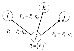
Figure 1: Transmission powers in terms of the power control and power allocation variables.

With appropriate scaling, we can always let $\hat{P}_{i}>1$ for all $i\in{\cal N}$ so that $\hat{S}_{i}>0$. Therefore, we have the following equivalent Throughput Optimal Power Control (TOPC) problem:

maximize

$$\sum_{(i,j)}b_{ij}^{*}\log\frac{Kh_{ij}(\hat{P}_{i})^{\gamma_{i}}\eta_{ij}}{\theta_{i}h_{ij}(\hat{P}_{i})^{\gamma_{i}}(1-\eta_{ij})+\displaystyle\sum_{m\neq i}h_{mj}(\hat{P}_{m})^{\gamma_{m}}+N_{j}}$$ (4)

subject to $$\eta_{ij}\geq 0,\quad\forall(i,j)\in{\cal E},$$

$$\sum_{j\in{\cal O}(i)}\eta_{ij}=1,~{}\gamma_{i}\leq 1,\quad\forall i\in{\cal N}.$$

III-C Conditions for Optimality

To solve the TOPC problem in (4), we compute the gradients of the objective function, denoted by $F$, with respect to the power allocation variables and the power control variables, respectively. They are as follows. For all $i\in{\cal N}$ and $j\in{\cal O}(i)$,

$$\frac{\partial F}{\partial\eta_{ij}} = P_{i}\left[\sum_{k\in{\cal O}(i)}b_{ik}^{*}\frac{-\theta_{i}h_{ik}}{IN_{ik}}\right.$$

$$\left.-\sum_{m\neq i}\sum_{k\in{\cal O}(m)}b_{mk}^{*}\frac{h_{ik}}{IN_{mk}}+\delta\eta_{ij}\right],$$

where the power allocation marginal gain indicator is

$$\delta\eta_{ij}\triangleq b_{ij}^{*}\left(\frac{1}{P_{ij}}+\frac{\theta_{i}h_{ij}}{IN_{ij}}\right).$$ (5)

For all $i\in{\cal N}$,

$$\frac{\partial F}{\partial\gamma_{i}}=\hat{S}_{i}\cdot\delta\gamma_{i},$$

where the power control marginal gain indicator is

$$\delta\gamma_{i} \triangleq P_{i}\left[\sum_{m\neq i}\sum_{k\in{\cal O}(m)}\frac{-b_{mk}^{*}h_{ik}}{IN_{mk}}+\right.$$ (6)

$$\left.\sum_{k\in{\cal O}(i)}\frac{-\theta_{i}b_{ik}^{*}h_{ik}}{IN_{ik}}+\sum_{k\in{\cal O}(i)}\delta\eta_{ik}\cdot\eta_{ik}\right].$$

The term $IN_{ij}$ appearing above is short-hand notation for the overall interference-plus-noise power at the receiver end of link $(i,j)$, that is

$$IN_{ij}=\theta_{i}h_{ij}\displaystyle\sum_{k\neq j}{e^{S_{ik}}}+\sum\limits_{m\neq i}{h_{mj}\sum_{k\in{\cal O}(m)}{e^{S_{mk}}}}+N_{j}.$$

The marginal gain indicators fully characterize the optimality conditions as follows.

Theorem 2

A feasible set of transmission power variables $\{\eta_{ik}\}_{(i,k)\in{\cal E}}$ and $\{\gamma_{i}\}_{i\in{\cal N}}$ is the solution of the TOPC problem (4) if and only if the following conditions hold. For all $i\in{\cal N}$, there exists a constant $\nu_{i}$ such that

$$\delta\eta_{ik}=\nu_{i}, \forall k\in{\cal O}(i),$$ (7)

$$\delta\gamma_{i}=0, \textrm{if}~{}\gamma_{i}<1,$$ (8)

$$\vspace{1mm}\delta\gamma_{i}\geq 0, \textrm{if}~{}\gamma_{i}=1.$$ (9)

Here, all $\eta_{ik}>0$ since $b_{ik}^{*}>0$ by assumption.

For the detailed proof of Theorem 2, see [13]. Due to the distributed form of the optimality conditions, every node can check the conditions with respect to its controlled variables locally, and adjust them towards the optimum. In the next section, we present a set of distributed algorithms that achieve the globally optimal power configuration.

III-D Distributed Power Control Algorithms

We design scaled gradient projection algorithms which iteratively update the nodes’ power allocation variables and power control variables in a distributed manner, so as to asymptotically converge to the optimal solution of (4). At each iteration, the variables are updated in the positive gradient direction, scaled by a positive definite matrix. When an update leads to a point outside the feasible set, the point is projected back into the feasible set [14].

III-D1 Power Allocation Algorithm (PA)

At the $k$th iteration at node $i$, the current local power allocation vector $\boldsymbol{\eta}_{i}^{k}=(\eta_{ij}^{k})_{j\in{\cal O}(i)}$ is updated by

$$\boldsymbol{\eta}_{i}^{k+1}=PA(\boldsymbol{\eta}_{i}^{k})=\left[\boldsymbol{\eta}_{i}^{k}+\beta_{i}^{k}\cdot(Q_{i}^{k})^{-1}\cdot\delta\boldsymbol{\eta}_{i}^{k}\right]_{Q_{i}^{k}}^{+}.$$

Here, $\delta\boldsymbol{\eta}_{i}^{k}=(\delta\eta_{ij}^{k})_{j\in{\cal O}(i)}$ and $\beta_{i}^{k}$ is a positive stepsize. The matrix $Q_{i}^{k}$ is symmetric, positive definite on the subspace $\{\boldsymbol{v}_{i}:\sum_{j\in{\cal O}(i)}{v_{ij}}=0\}$. Finally, $[\cdot]_{Q_{i}^{k}}^{+}$ denotes the projection on the feasible set of $\boldsymbol{\eta}_{i}$ relative to the norm induced by $Q_{i}^{k}$.

Suppose each node $j$ can measure the value of $SINR_{ij}$ for any of its incoming links. Before an iteration of $PA$, node $i$ collects the current $SINR_{ij}$’s via feedback from its next-hop neighbors $j$. Node $i$ can then readily compute all $\delta\eta_{ij}$’s according to

$$\delta\eta_{ij}=b_{ij}^{*}\left(\frac{1}{P_{ij}}+\frac{\theta_{i}h_{ij}}{IN_{ij}}\right)=\frac{b_{ij}^{*}}{P_{ij}}\left(1+\frac{\theta_{i}SINR_{ij}}{K}\right).$$

Note that since the calculation of $\delta\eta_{ij}$ involves only locally obtainable measures, the $PA$ algorithm does not require global exchange of control messages.

III-D2 Power Control Algorithm (PC)

After a phase for exchanging control messages (which will be discussed below), every node $i$ is able to calculate its power control marginal gain indicator $\delta\gamma_{i}$. From a network-wide viewpoint, the power control vector $\boldsymbol{\gamma}^{k}=(\gamma_{i}^{k})_{i\in{\cal N}}$ is updated by

$$\boldsymbol{\gamma}^{k+1}=PC(\boldsymbol{\gamma}^{k})=\left[\boldsymbol{\gamma}^{k}+\xi^{k}\cdot(V^{k})^{-1}\cdot\delta\boldsymbol{\gamma}^{k}\right]_{V^{k}}^{+}.$$

Here, $\xi^{k}$ is a positive stepsize and matrix $V^{k}$ is symmetric and positive definite. Note that $PC$ becomes amenable to distributed implementation if and only if $V^{k}$ is diagonal.

We now derive an efficient protocol which allows each node to calculate its own $\delta\gamma_{i}$ given limited control messaging. We first re-order the summations on the RHS of (6) as

$$\delta\gamma_{i}=P_{i}\left[\sum_{j\neq i}\left\{-h_{ij}\sum_{m\in{\cal I}(j)}{\frac{b_{mj}^{*}}{IN_{mj}}}\right\}\right.$$

$$\left.\sum_{j\in{\cal O}(i)}\left\{b_{ij}^{*}\left[\frac{1}{P_{i}}+(\theta_{i}\eta_{ij}-\theta_{i}+1)\frac{h_{ij}}{IN_{ij}}\right]\right\}\right].$$

With reference to the above expression, we propose the following procedure for computing $\delta\gamma_{i}$.

Power Control Message Exchange Protocol: Let each node $j$ assemble the measures $\frac{b_{mj}^{*}}{IN_{mj}}$ from all its incoming links $(m,j)$. For this purpose, an upstream neighbor $m$ needs to inform $j$ of the value $b_{mj}^{*}/P_{mj}$. Since node $j$ can measure both $SINR_{mj}$ and $h_{mj}$, it can calculate

$$\frac{b_{mj}^{*}}{IN_{mj}}=\frac{b_{mj}^{*}}{P_{mj}}\frac{SINR_{mj}}{h_{mj}K}.$$

After obtaining the measures from all incoming links, node $j$ sums them up to form the power control message:

$$Msg(j)\triangleq\sum_{m\in{\cal I}(j)}{\frac{b_{mj}^{*}}{IN_{mj}}}.$$

It then broadcasts $Msg(j)$ to the whole network. The process for control messaging is illustrated by Figure 2, where the solid arrows represent local message communication and the hollow arrow signifies the broadcasting of the message.

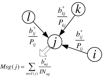
Figure 2: Information Exchange Protocol for Power Control Algorithm

Upon obtaining $Msg(j)$ from node $j\neq i$, node $i$ processes it according to the following rule. If $j$ is a next-hop neighbor of $i$, it multiplies the message with $h_{ij}$ and subtracts the product from the local measure

$$b_{ij}^{*}\left[\frac{1}{P_{i}}+(\theta_{i}\eta_{ij}-\theta_{i}+1)\frac{h_{ij}}{IN_{ij}}\right]$$

$$= \delta\eta_{ij}\cdot\eta_{ij}+\left(\delta\eta_{ij}-\frac{b_{ij}^{*}}{P_{ij}}\right)\frac{1-\theta_{i}}{\theta_{i}}.$$

Otherwise, it multiplies $Msg(j)$ with $-h_{ij}$. Finally, node $i$ adds up the results derived from processing all other nodes’ messages, and this sum multiplied by $P_{i}$ equals $\delta\gamma_{i}$. Note that in a symmetric duplex channel, $h_{ij}\approx h_{ji}$, and node $i$ may use its own measure of $h_{ji}$ in place of $h_{ij}$. Otherwise, it will need channel feedback from node $j$ to calculate $h_{ij}$. To summarize, the protocol requires only one message from each node to be broadcast to the whole network.

III-D3 Convergence of Algorithms

We now formally state the central convergence result for the $PA$ and $PC$ algorithms discussed above.

Theorem 3

From any feasible initial transmission power configuration $\{\boldsymbol{\eta}_{i}^{0}\}$ and $\boldsymbol{\gamma}^{0}$, there exist valid scaling matrices $\{Q_{i}^{k}\}$ and $V^{k}$, and positive stepsizes $\{\beta_{i}^{k}\}$ and $\xi^{k}$ such that the sequences generated by the algorithms $PA(\cdot)$ and $PC(\cdot)$ converge, i.e., $\boldsymbol{\eta}_{i}^{k}\to\boldsymbol{\eta}_{i}^{*}$ for all $i$, and $\boldsymbol{\gamma}^{k}\to\boldsymbol{\gamma}^{*}$ as $k\to\infty$. Furthermore, $\{\boldsymbol{\eta}_{i}^{*}\}$ and $\boldsymbol{\gamma}^{*}$ constitute a set of jointly optimal solution to the TOPC problem (4).

In the $PA$ and $PC$ algorithms, the scaling matrices are chosen to be appropriate diagonal matrices which approximate the relevant Hessians such that the objective value is increased by every iteration until the optimum is achieved. This allows the scaled gradient projection algorithms to approximate constrained Newton algorithms, which are known to have fast convergence rates. Furthermore, the scaling matrices are shown to be easily calculated at each node using very limited control messaging. The detailed derivation of these parameters and the full proof of Theorem 3 can be found in [13].

Also note that the convergence of the algorithms does not require any particular order of running $PA$ and $PC$ algorithms at different nodes. Any node $i$ only needs to update its own variables $\boldsymbol{\eta}_{i}$ and $\gamma_{i}$ using $PA$ and $PC$ until its local variables satisfy the optimality conditions (7)-(9).

IV Throughput Optimality of Iterative Maximum Differential Backlog Policy

Since the $PA$ and $PC$ algorithms need a certain number of iterations before reaching a close neighborhood of an optimum to the problem in (4), the optimal service rates dictated by the MDB policy cannot be applied instantaneously. Rather the optimal service rates can only be found iteratively over time. At any moment in the convergence interval, the queues are served at the rates which are iteratively updated towards the optimal rates for the queue state at the beginning of a slot. The service rates obtained at the end of a convergence period are optimal only for the queue state some time ago. The effect of using lagging optimal service rates is studied in the context of $N\times N$ packet switches by Neely et al. [15] and in a queueing network with Poisson arrivals and exponential service rates by Tassiulas and Ephremides [16]. In [15, 16], however, the process of finding the optimal rates is not iterative. It is assumed that once the (outdated) queue state information becomes available, the optimal rates are obtained instantaneously. Here, we analyze the iterative MDB algorithm with convergence time in general multi-hop networks with i.i.d. random arrival processes and general rate regions. We show that the throughput optimality of the MDB policy is preserved for any finite convergence time. For this, we invent a new geometric approach for computing the expected Lyapunov drift of the queue state.

IV-A Transient Optimal Rates

Without loss of generality, assume the convergence time of the MDB algorithms in Section III-D is the length of a time slot $T$, i.e., at time $\tau=(t+1)T$, the optimal service rate vector for $\boldsymbol{U}[t]$ is achieved. For ease of analysis, we further scale time so that $T=1$.

We assume a general feasible service rate region. Instead of studying the service rates $(R_{ij}^{k}(\tau))$, in this section we focus on the virtual service rates. First define the instantaneous virtual service rate of queue $i^{k}$ by

$$\tilde{R}_{i}^{k}(\tau)=\sum_{j\in{\cal O}(i)}R_{ij}^{k}(\tau)-\sum_{m\in{\cal I}(i)}R_{mi}^{k}(\tau).$$

Such a transformation considerably simplifies our subsequent analysis. The vector of virtual service rates over the $t$th slot is

$$\tilde{\boldsymbol{R}}[t]=\int_{t}^{t+1}\tilde{\boldsymbol{R}}(\tau)d\tau,$$

where the integration is taken component-wise. By definition, we have $\tilde{R}_{i}^{k}[t]=\sum_{j\in{\cal O}(i)}R_{ij}^{k}[t]-\sum_{m\in{\cal I}(i)}R_{mi}^{k}[t]$. Therefore, we consider $\tilde{\boldsymbol{R}}[t]=(\tilde{R}_{i}^{k}[t])_{i\in{\cal N},k\in{\cal K}}$ induced by $\boldsymbol{R}[t]$. A virtual service rate vector over a slot $\tilde{\boldsymbol{R}}[t]$ is feasible if it is induced by a feasible $\boldsymbol{R}[t]\in{\cal C}(\Pi)$. Denote the set of all feasible $\tilde{\boldsymbol{R}}[t]$ by ${\cal C}_{\tilde{\boldsymbol{R}}}(\Pi)$. It is straightforward to verify that ${\cal C}_{\tilde{\boldsymbol{R}}}(\Pi)$ is compact and convex. By Theorem 1 of [3], the subset of ${\cal C}_{\tilde{\boldsymbol{R}}}(\Pi)$ in the positive orthant is the stability region of the wireless multi-hop networks with power constraints $\Pi$. For brevity, we denote ${\cal C}_{\tilde{\boldsymbol{R}}}(\Pi)$ by ${\cal C}$ in this section. Finally, the queueing dynamics in (1) can be written in vector form as

$$\boldsymbol{U}[t+1]\leq\left(\boldsymbol{U}[t]-\tilde{\boldsymbol{R}}[t]+\boldsymbol{B}[t]\right)^{+}.$$ (10)

Note that maximizing the MDB objective function (2) in $\boldsymbol{R}$ over the feasible service rate region ${\cal C}(\Pi)$ is equivalent to maximizing $\boldsymbol{U}[t]^{\prime}\cdot\tilde{\boldsymbol{R}}$ in $\tilde{\boldsymbol{R}}$ over the virtual service rate region ${\cal C}$. We denote the maximizing $\tilde{\boldsymbol{R}}$ by $\tilde{\boldsymbol{R}}^{*}(\boldsymbol{U}[t])$. From now on, we simply call $\tilde{\boldsymbol{R}}$ the service rate vector and refer to $\tilde{\boldsymbol{R}}^{*}(\boldsymbol{U}[t])$ as the optimal rate allocation for queue state $\boldsymbol{U}[t]$.

Recall our discussion of the distributed MDB control algorithms in the last section. Due to the iterative nature of the algorithms, the optimal power vector and the optimal rate allocation for a given queue state can be found only when the algorithms converge. Therefore in practice, the rate vector solving (2) for $(b_{ij}^{*}[t])$ cannot be applied instantly at the beginning of the $t$th slot. The actual service rates $\tilde{\boldsymbol{R}}(\tau),\tau\in\mathbb{R}_{+}$, are always in transience, shifting from the previous optimum to the next optimum. Thus, the instantaneous rate vector at time $\tau=t$ is $\tilde{\boldsymbol{R}}(t)=\tilde{\boldsymbol{R}}^{*}(\boldsymbol{U}[t-1])$, and at time $\tau=t+1$, $\tilde{\boldsymbol{R}}(t+1)=\tilde{\boldsymbol{R}}^{*}(\boldsymbol{U}[t])$.

IV-B Lyapunov Drift Criterion

Following the previous model, the process $\left\{\left(\boldsymbol{U}[t],\boldsymbol{U}[t-1]\right)\right\}_{t=1}^{\infty}$ forms a Markov chain. The state $\left(\boldsymbol{U}[t],\boldsymbol{U}[t-1]\right)\triangleq\boldsymbol{W}[t]$ lies in the state space ${\cal W}=\mathbb{R}_{+}^{M}\times\mathbb{R}_{+}^{M}$ where $M$ is the total number of queues. As an extension of Foster’s criterion for a recurrent Markov chain [17], the following condition is used in studying the stability of stochastic queueing systems [1, 15].

Lemma 1

[1] If there exist a (Lyapunov) function $V:{\cal W}\mapsto\mathbb{R}_{+}$, a compact subset ${\cal W}_{0}\subset{\cal W}$, and a positive constant $\varepsilon_{0}$ such that for all $\boldsymbol{w}\in{\cal W}_{0}$

$$\mathbb{E}\left[V(\boldsymbol{W}[t+1])-V(\boldsymbol{W}[t])|\boldsymbol{W}[t]=\boldsymbol{w}\right]<\infty,$$ (11)

and for all $\boldsymbol{w}\notin{\cal W}_{0}$

$$\mathbb{E}\left[V(\boldsymbol{W}[t+1])-V(\boldsymbol{W}[t])|\boldsymbol{W}[t]=\boldsymbol{w}\right]\leq-\varepsilon_{0},$$ (12)

then the Markov chain $\{\boldsymbol{W}[t]\}$ is recurrent. Hence, the queueing system is stable in the sense of Definition 1.

We use the Lyapunov function from [16]:

$$V(\boldsymbol{W}[t]) = \sum_{k\in{\cal K}}\sum_{i\in{\cal N}}U_{i}^{k}[t]^{2}+(U_{i}^{k}[t]-U_{i}^{k}[t-1])^{2}$$

$$= \|\boldsymbol{U}[t]\|^{2}+\|\boldsymbol{U}[t]-\boldsymbol{U}[t-1]\|^{2},$$

where $\|\cdot\|$ denotes the $L^{2}$ norm. Using relation (10), we derive the following upper bound on the expected one-step Lyapunov drift conditioned on $\boldsymbol{W}[t]=\left(\boldsymbol{u}_{t},\boldsymbol{u}_{t-1}\right)$:

$$\mathbb{E}\left[V(\boldsymbol{W}[t+1])-V(\boldsymbol{W}[t])|\boldsymbol{W}[t]=\left(\boldsymbol{u}_{t},\boldsymbol{u}_{t-1}\right)\right]$$

$$\leq 2\boldsymbol{u}_{t}^{\prime}\left(\boldsymbol{a}-\tilde{\boldsymbol{R}}[t]\right)+2\left(|\boldsymbol{b}|+\|\tilde{\boldsymbol{R}}[t]\|^{2}\right)$$

$$-\|\boldsymbol{u}_{t}-\boldsymbol{u}_{t-1}\|^{2},$$

where $\boldsymbol{b}$ is the vector of second moments of the random arrival rates and $|\cdot|$ denotes the $L^{1}$ norm. The detailed derivation of the above inequality is left to Appendix -A.

Because the distributed power adjustment algorithms in Section III-D increase the objective value $\boldsymbol{u}_{t}^{\prime}\cdot\tilde{\boldsymbol{R}}$ with every iteration from time $t$ to $t+1$, $\boldsymbol{u}_{t}^{\prime}\cdot\tilde{\boldsymbol{R}}(\tau)$ is increasing in $\tau\in[t,t+1)$ and given $\boldsymbol{W}[t]=\left(\boldsymbol{u}_{t},\boldsymbol{u}_{t-1}\right)$,

$$\boldsymbol{u}_{t}^{\prime}\cdot\tilde{\boldsymbol{R}}[t]=\int_{t}^{t+1}\boldsymbol{u}_{t}^{\prime}\cdot\tilde{\boldsymbol{R}}(\tau)d\tau\geq$$

$$\int_{t}^{t+1}\boldsymbol{u}_{t}^{\prime}\cdot\tilde{\boldsymbol{R}}(t)d\tau=\boldsymbol{u}_{t}^{\prime}\cdot\tilde{\boldsymbol{R}}(t)=\boldsymbol{u}_{t}^{\prime}\cdot\tilde{\boldsymbol{R}}^{*}(\boldsymbol{u}_{t-1}).$$

Also notice that because the second moment vector $\boldsymbol{b}$ is assumed to be finite and $\tilde{\boldsymbol{R}}[t]$ lies in the bounded region ${\cal C}$, we can find a finite constant $\lambda$ such that $2\left(|\boldsymbol{b}|+\|\tilde{\boldsymbol{R}}[t]\|^{2}\right)\leq\lambda$. Thus, the conditional expected Lyapunov drift is upper bounded by

$$2\boldsymbol{u}_{t}^{\prime}\cdot\left(\boldsymbol{a}-\tilde{\boldsymbol{R}}^{*}(\boldsymbol{u}_{t-1})\right)-\|\boldsymbol{u}_{t}-\boldsymbol{u}_{t-1}\|^{2}+\lambda.$$

Using the above Lyapunov function and the upper bound for the expected Lyapunov drift, we show the following main result.

Theorem 4

The iterative MDB policy with convergence time is throughput optimal, i.e. it stabilizes all arrival processes whose average rate vector $\boldsymbol{a}\in\mathbf{int}~{}{\cal C}$.

Guided by the Lyapunov drift criterion, the proof aims to find an $\varepsilon_{0}>0$ and a compact set ${\cal W}_{0}$ (which may depend on $\varepsilon_{0}$) which satisfy the conditions (11)-(12) for any average arrival rates $\boldsymbol{a}\in\mathbf{int}~{}{\cal C}$. Note that condition (11) is always satisfied since the first and second moments of arrival rates as well as the service rate vector are bounded. Now consider the compact region characterized by

$${\cal W}_{0}=\{\boldsymbol{w}\in\mathbb{R}_{+}^{M}\times\mathbb{R}_{+}^{M}:V(\boldsymbol{w})\leq\Omega\}.$$ (13)

Given $\varepsilon_{0}>0$, we need to specify a finite $\Omega$ and show that when $\boldsymbol{w}[t]=(\boldsymbol{u}_{t},\boldsymbol{u}_{t-1})\notin{\cal W}_{0}$,

$$2\boldsymbol{u}_{t}^{\prime}\cdot\left(\boldsymbol{a}-\tilde{\boldsymbol{R}}^{*}(\boldsymbol{u}_{t-1})\right)-\|\boldsymbol{u}_{t}-\boldsymbol{u}_{t-1}\|^{2}+\lambda\leq-\varepsilon_{0}.$$ (14)

Towards this objective, we devise a geometric method to relate the position of $\boldsymbol{u}_{t}$ and $\boldsymbol{u}_{t-1}$ in the state space to the value of the inner product $\boldsymbol{u}_{t}^{\prime}\cdot[\boldsymbol{a}-\tilde{\boldsymbol{R}}^{*}(\boldsymbol{u}_{t-1})]$. In order to reveal the insight underlying this approach, we first develop the methodology in $\mathbb{R}^{2}$. The generalization to higher dimensions as well as the proof for Theorem 4 can be found in Appendix -B and -C.

IV-C Geometric Analysis

In this section, we analyze vectors of arrival rates, service rates, and queue states geometrically. In view of condition (14), we characterize a neighborhood around $\boldsymbol{u}_{t}$ which has the following properties: if $\boldsymbol{u}_{t-1}$ lies in the neighborhood, then the first term $2\boldsymbol{u}_{t}^{\prime}\cdot(\boldsymbol{a}-\tilde{\boldsymbol{R}}^{*}(\boldsymbol{u}_{t-1}))$ is substantially negative ($\leq-\lambda-\varepsilon_{0}$); if $\boldsymbol{u}_{t-1}$ lies outside the neighborhood (meaning that $\|\boldsymbol{u}_{t}-\boldsymbol{u}_{t-1}\|^{2}$ is relatively large), then the second term $-\|\boldsymbol{u}_{t}-\boldsymbol{u}_{t-1}\|^{2}$ is sufficiently negative for (14) to hold.

We assume an average arrival rate vector $\boldsymbol{a}\in\mathbf{int}~{}{\cal C}$. There must exist a point $\bar{\boldsymbol{a}}\in\mathbf{bd}~{}{\cal C}$, and a positive constant $\varepsilon$ such that $\boldsymbol{a}+\varepsilon\cdot\boldsymbol{1}\leq\bar{\boldsymbol{a}}$. Therefore the point $\boldsymbol{e}=\boldsymbol{a}+\frac{\varepsilon}{2}\cdot\bf 1$ is also in the interior of ${\cal C}$.

Given the current queue state vector $\boldsymbol{u}_{t}\geq\boldsymbol{0}$, the hyperplane ${\cal B}_{\boldsymbol{e}}(\boldsymbol{u}_{t})\triangleq\{\boldsymbol{x}:\boldsymbol{u}_{t}^{\prime}\cdot\boldsymbol{x}=\boldsymbol{u}_{t}^{\prime}\cdot\boldsymbol{e}\}$ is perpendicular to $\boldsymbol{u}_{t}$ and crosses the point $\boldsymbol{e}$. The intersection of halfspace ${\cal H}_{\boldsymbol{e}}^{+}(\boldsymbol{u}_{t})\triangleq\{\boldsymbol{x}:\boldsymbol{u}_{t}^{\prime}\cdot\boldsymbol{x}\geq\boldsymbol{u}_{t}^{\prime}\cdot\boldsymbol{e}\}$ with ${\cal C}$, denoted by ${\cal C}_{\boldsymbol{e}}^{+}(\boldsymbol{u}_{t})$, is closed and convex with non-empty interior [18].

Lemma 2

For $\boldsymbol{y}\in{\cal C}_{\boldsymbol{e}}^{+}(\boldsymbol{u}_{t})$, $\boldsymbol{u}_{t}^{\prime}\cdot[\boldsymbol{a}-\boldsymbol{y}]\leq-\frac{\varepsilon}{2}\|\boldsymbol{u}_{t}\|$.

Proof: Since $\boldsymbol{y}\in{\cal H}_{\boldsymbol{e}}^{+}(\boldsymbol{u}_{t})$, by definition $\boldsymbol{u}_{t}^{\prime}\cdot\boldsymbol{y}\geq\boldsymbol{u}_{t}^{\prime}\cdot\boldsymbol{e}$. Thus,

$$\boldsymbol{u}_{t}^{\prime}\cdot[\boldsymbol{a}-\boldsymbol{y}] \leq \boldsymbol{u}_{t}^{\prime}\cdot[\boldsymbol{a}-\boldsymbol{e}]$$

$$= -\frac{\varepsilon}{2}|\boldsymbol{u}_{t}|\leq-\frac{\varepsilon}{2}\|\boldsymbol{u}_{t}\|.$$

The last inequality follows from $|\boldsymbol{u}_{t}|\geq\|\boldsymbol{u}_{t}\|$ since $\boldsymbol{u}_{t}\geq\boldsymbol{0}$. ∎

Two-Dimensional Heuristic

Assume there are two queues in the network and index them by $1$ and $2$. In this subsection, all vectors, hyperplanes, surfaces, etc. are in $\mathbb{R}^{2}$. The hyperplane ${\cal B}_{\boldsymbol{e}}(\boldsymbol{u}_{t})$ must intersect $\mathbf{bd}~{}{\cal C}$ at two different points, as illustrated in Figure 3.

Figure 3: The geometry when ${\cal B}_{\boldsymbol{e}}(\boldsymbol{u}_{t})$ intersects $\mathbf{bd}~{}{\cal C}$ at two different points in $\mathbb{R}_{2}^{+}$

Let the two points be $\boldsymbol{f}_{1}$ and $\boldsymbol{f}_{2}$, where $\boldsymbol{f}_{1}$ is the upper-left one. Denote the hyperplane (which is a line in $\mathbb{R}^{2}$) tangent to ${\cal C}$ at $\boldsymbol{f}_{1}$ by ${\cal B}_{\boldsymbol{f}_{1}}(\boldsymbol{n}_{1})$, where $\boldsymbol{n}_{1}$ is the unit normal vector of the tangent line. Specifically, we require $\boldsymbol{n}_{1}$ to be pointing outward from ${\cal C}$. Since ${\cal C}$ is not confined in $\mathbb{R}_{+}^{2}$, $\boldsymbol{f}_{1}$ is not necessarily nonnegative, and neither is $\boldsymbol{n}_{1}$. If there exist multiple tangent lines at $\boldsymbol{f}_{1}$, take $\boldsymbol{n}_{1}$ to be any one of them. Let the unit normal vector at $\boldsymbol{f}_{2}$ be $\boldsymbol{n}_{2}$, defined in the same manner. Let

$$\theta_{1}(\overrightarrow{\boldsymbol{u}_{t}})=\arccos(\boldsymbol{n}_{1}^{\prime}\cdot\overrightarrow{\boldsymbol{u}_{t}}),~{}~{}\theta_{2}(\overrightarrow{\boldsymbol{u}_{t}})=\arccos(\boldsymbol{n}_{2}^{\prime}\cdot\overrightarrow{\boldsymbol{u}_{t}}),$$

where $\overrightarrow{\boldsymbol{u}_{t}}$ stands for the normalized vector of $\boldsymbol{u}_{t}$. Since $\boldsymbol{e}\in\mathbf{int}~{}{\cal C}$, $\boldsymbol{n}_{1}$ and $\boldsymbol{n}_{2}$ can never be parallel to $\overrightarrow{\boldsymbol{u}_{t}}$. Thus,

$$\boldsymbol{n}_{1}^{\prime}\cdot\overrightarrow{\boldsymbol{u}_{t}}<1,\quad\quad\boldsymbol{n}_{2}^{\prime}\cdot\overrightarrow{\boldsymbol{u}_{t}}<1,$$

and $\theta_{1}(\overrightarrow{\boldsymbol{u}_{t}})>0$, $\theta_{2}(\overrightarrow{\boldsymbol{u}_{t}})>0$. Moreover, $\theta_{1}(\overrightarrow{\boldsymbol{u}_{t}})$ and $\theta_{2}(\overrightarrow{\boldsymbol{u}_{t}})$ are bounded away from zero for all $\boldsymbol{u}_{t}$. To see this, we make use of Figure 3 again. The point $\boldsymbol{f}_{e}$ is on the boundary and the vector $\boldsymbol{f}_{e}-\boldsymbol{e}$ is parallel to $\boldsymbol{u}_{t}$. By simple geometry, the convexity of the rate region implies $\theta_{1}(\boldsymbol{u}_{t})\geq\arctan(\|\boldsymbol{f}_{e}-\boldsymbol{e}\|/\|\boldsymbol{f}_{1}-\boldsymbol{e}\|)$. Because $\boldsymbol{e}$ is an interior point, $\|\boldsymbol{f}_{e}-\boldsymbol{e}\|\geq\xi>0$. Moreover, $\|\boldsymbol{f}_{1}-\boldsymbol{e}\|\leq D<\infty$ since ${\cal C}$ is a bounded region. Therefore, $\theta_{1}(\overrightarrow{\boldsymbol{u}_{t}})\geq\arctan(\xi/D)>0$. The same is true for $\theta_{2}(\overrightarrow{\boldsymbol{u}_{t}})$. Thus, we can construct a non-empty cone emanating from the origin sweeping from the direction of vector $\boldsymbol{u}_{t}$ clockwise by $\theta_{2}(\overrightarrow{\boldsymbol{u}_{t}})$ and counterclockwise by $\theta_{1}(\overrightarrow{\boldsymbol{u}_{t}})$. Such a cone always contains $\boldsymbol{u}_{t}$ in its strict interior. This is illustrated in Figure 4.

We consider the following two cases. First, if $\|\boldsymbol{u}_{t}-\boldsymbol{u}_{t-1}\|/\|\boldsymbol{u}_{t}\|\leq\sin\left[\min\{\theta_{1}(\overrightarrow{\boldsymbol{u}_{t}}),\theta_{2}(\overrightarrow{\boldsymbol{u}_{t}}),\pi/2\}\right]\equiv\alpha(\overrightarrow{\boldsymbol{u}_{t}})$, then the pair of points $\left(\boldsymbol{u}_{t},\boldsymbol{u}_{t-1}\right)$ both lie in the cone described above. In this case, $\boldsymbol{u}_{t-1}$ is said to be in the neighborhood of $\boldsymbol{u}_{t}$. See Figure 4.

Figure 4: The geometry of $\boldsymbol{u}_{t-1}$ lying in the neighborhood of $\boldsymbol{u}_{t}$, where $r=\|\boldsymbol{u}_{t}\|\cdot\alpha(\vec{\boldsymbol{u}}_{t})$.

Let $\alpha$ be the infimum of $\alpha(\overrightarrow{\boldsymbol{u}_{t}})$ over all nonnegative unit vector $\overrightarrow{\boldsymbol{u}_{t}}$. Because all $\theta_{1}(\overrightarrow{\boldsymbol{u}_{t}})$ and $\theta_{2}(\overrightarrow{\boldsymbol{u}_{t}})$ are strictly positive, $\alpha$ must be strictly positive. If $\|\boldsymbol{u}_{t}-\boldsymbol{u}_{t-1}\|/\|\boldsymbol{u}_{t}\|\leq\alpha$, $\boldsymbol{u}_{t-1}$ is also in the cone with $\boldsymbol{u}_{t}$. In this case, the hyperplane of normal vector $\boldsymbol{u}_{t-1}$ tangent to the rate region ${\cal C}$ touches $\mathbf{bd}~{}{\cal C}$ at $\tilde{\boldsymbol{R}}^{*}(\boldsymbol{u}_{t-1})$ somewhere between $\boldsymbol{f}_{1}$ and $\boldsymbol{f}_{2}$, i.e., $\tilde{\boldsymbol{R}}^{*}(\boldsymbol{u}_{t-1})\in{\cal C}_{\boldsymbol{e}}^{+}(\boldsymbol{u}_{t})$. By Lemma 2, the inner product $\boldsymbol{u}_{t}^{\prime}\cdot[\boldsymbol{a}-\tilde{\boldsymbol{R}}^{*}(\boldsymbol{u}_{t-1})]\leq-\frac{\varepsilon}{2}\|\boldsymbol{u}_{t}\|$. Then for all $\boldsymbol{w}[t]$ such that $V(\boldsymbol{w}[t])>(1+\alpha^{2})\cdot(\varepsilon_{0}+\lambda)^{2}/\varepsilon^{2}\equiv\Omega_{1}$, $\|\boldsymbol{u}_{t}\|>(\varepsilon_{0}+\lambda)/\varepsilon$, and therefore

$$2\boldsymbol{u}_{t}^{\prime}\cdot\left(\boldsymbol{a}-\tilde{\boldsymbol{R}}^{*}(\boldsymbol{u}_{t-1})\right)-\|\boldsymbol{u}_{t}-\boldsymbol{u}_{t-1}\|^{2}+\lambda$$

$$\leq 2\boldsymbol{u}_{t}^{\prime}\cdot\left(\boldsymbol{a}-\tilde{\boldsymbol{R}}^{*}(\boldsymbol{u}_{t-1})\right)+\lambda<-\varepsilon_{0},$$

which is the desired condition (14).

If $\|\boldsymbol{u}_{t}-\boldsymbol{u}_{t-1}\|/\|\boldsymbol{u}_{t}\|>\alpha$ and assume $\|\boldsymbol{u}_{t}-\boldsymbol{u}_{t-1}\|^{2}=\omega$, then

$$2\boldsymbol{u}_{t}^{\prime}\cdot\left(\boldsymbol{a}-\tilde{\boldsymbol{R}}^{*}(\boldsymbol{u}_{t-1})\right)-\|\boldsymbol{u}_{t}-\boldsymbol{u}_{t-1}\|^{2}+\lambda$$

$$\leq 2\|\boldsymbol{u}_{t}\|\|\boldsymbol{a}-\tilde{\boldsymbol{R}}^{*}(\boldsymbol{u}_{t-1})\|-\omega+\lambda$$

$$< 2\sqrt{\omega/\alpha^{2}}\sqrt{\lambda/2}-\omega+\lambda$$

$$= \sqrt{2\omega\lambda}/\alpha-\omega+\lambda.$$

Define

$$\omega_{2}=\inf\{\omega>0:\sqrt{2\omega\lambda}/\alpha-\omega+\lambda\leq-\varepsilon_{0}\}.$$ (15)

Then for all $\boldsymbol{w}[t]$ such that $V(\boldsymbol{w}[t])>(1+1/\alpha^{2})\omega_{2}\equiv\Omega_{2}$, $\|\boldsymbol{u}_{t}-\boldsymbol{u}_{t-1}\|^{2}>\omega_{2}$ and (14) holds.

Combining the above two cases and letting $\Omega=\max\{\Omega_{1},\Omega_{2}\}$, we see that the region specified in (13) satisfies Lemma 1 and Theorem 4 follows.

V Numerical Experiments

To assess the practical performance of the node-based distributed MDB policy in stochastic wireless networks, we conduct the following simulation to compare the total backlogs resulting from the same arrival processes under different MDB schemes.

Our scheme iteratively adjusts the transmission powers during a slot to find the optimal rates for the queue state at the beginning of a slot. As a consequence, the MDB optimization is done with delayed queue state information, the transmission rates keep changing with time, and the optimal rates are achieved only at the end (beginning) of the current (next) slot. Recently, Giannoulis et al. [9] proposed another distributed power control algorithm to implement the MDB policy in CDMA networks. Instead of converging to the optimal solution for the current MDB problem, their scheme updates the link powers based on the present queue state only once in a slot. The new queue state at the beginning of the next slot is used for the subsequent iteration. To highlight the above difference, we refer to our method as “iterative MDB with convergence”, and the method studied in [9] as “iterative MDB without convergence”. Both schemes are shown to preserve the throughput optimality of the original MDB policy, which ideally (instantaneously) finds the optimal transmission rates for the queue state at the beginning of a slot, and applies them for the whole slot.

For a single run of the experiment, we use a network with $N$ nodes uniformly distributed in a disc of unit radius. Nodes $i$ and $j$ share a link if their distance $d(i,j)$ is less than $2.5/\sqrt{N}$, so that the average number of a node’s neighbors remains constant with $N$. The path gain is modeled as $h_{ij}=d(i,j)^{-4}$. The processing gain of the CDMA system is $K=10^{5}$, and the self-interference parameter is $\theta_{i}=0.25$. All nodes are subject to the common total power constraint $\hat{P}_{i}=100$ and AWGN of power $N_{i}=0.1$.

Each node is the source node of one session with the destination chosen from the other $N-1$ nodes at random. At the beginning of every slot, the new arrivals of all $N$ sessions are independent Poisson random variables with the same parameter $B$. As an approximation, we assume the iterative MDB scheme converges after 50 iterations of the $PA$ and $PC$ algorithms. The convergence time is taken to be the length of a slot, as in Section IV. The network performance is investigated under each of the MDB schemes with the same set of arrival processes. The total backlog in the network is recorded after every slot. Figure 5 shows the backlog curves generated by the three schemes after averaging $10$ independent runs with the parameters $N=10$ and $B=4$.

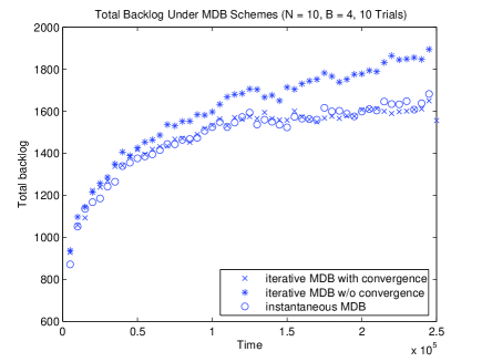
Figure 5: Total backlogs under three MDB schemes ($N=10,B=4$).

Figure 6 reports the result from the experiment with the parameters $N=5$ and $B=7$.

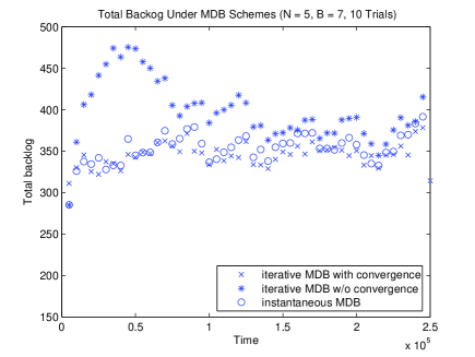
Figure 6: Total backlogs under three MDB schemes ($N=5,B=7$).

The three methods all manage to stabilize the network queues in the long run. However, the iterative MDB scheme with convergence and the instantaneous MDB scheme result in lower queue occupancy, hence lower delay, than the iterative MDB scheme without convergence.

VI Conclusion

In this work, we study the distributed implementation of the Maximum Differential Backlog algorithm within interference-limited CDMA wireless networks with random traffic arrivals. In the first half of the paper, we develop a set of node-based iterative power allocation and power control algorithms for solving the MDB optimization problem. Our algorithms are based on the scaled gradient projection method. We show that the algorithms can solve the MDB optimization in a distributed manner using low communication overhead. Because these iterative algorithms typically require non-negligible time to converge, the optimal rate allocation can only be found iteratively over time. In the second half of the paper, we analyze the iterative MDB policy with convergence time. Using a new geometric approach for analysis of the expected Lyapunov drift, we prove that throughput optimality of the MDB algorithm still holds as long as the second moments of traffic arrival rates are bounded. The two parts of the paper in conjunction yield a distributed solution to throughput optimal control of CDMA wireless networks with random traffic arrivals.

-A Derivation of Lyapunov Drift

By definition, the difference of Lyapunov values $V(\boldsymbol{W}[t+1])$ and $V(\boldsymbol{W}[t])$ can be written as

$$V(\boldsymbol{W}[t+1])-V(\boldsymbol{W}[t])$$

$$= \|\boldsymbol{U}[t+1]\|^{2}-\|\boldsymbol{U}[t]\|^{2}+\|\boldsymbol{U}[t+1]-\boldsymbol{U}[t]\|^{2}$$

$$-\|\boldsymbol{U}[t]-\boldsymbol{U}[t-1]\|^{2}$$

$$= 2\boldsymbol{U}[t+1]^{\prime}\cdot\left(\boldsymbol{U}[t+1]-\boldsymbol{U}[t]\right)$$

$$-\|\boldsymbol{U}[t]-\boldsymbol{U}[t-1]\|^{2}.$$

Using relation (10), we have

$$\boldsymbol{U}[t+1]^{\prime}\cdot\left(\boldsymbol{U}[t+1]-\boldsymbol{U}[t]\right)$$

$$\leq \left(\left(\boldsymbol{U}[t]-\tilde{\boldsymbol{R}}[t]+\boldsymbol{B}[t]\right)^{+}\right)^{\prime}\cdot$$

$$\left(\left(\boldsymbol{U}[t]-\tilde{\boldsymbol{R}}[t]+\boldsymbol{B}[t]\right)^{+}-\boldsymbol{U}[t]\right)$$

$$\leq \left(\boldsymbol{U}[t]-\tilde{\boldsymbol{R}}[t]+\boldsymbol{B}[t]\right)^{\prime}\cdot\left(\boldsymbol{B}[t]-\tilde{\boldsymbol{R}}[t]\right)$$

$$\leq \boldsymbol{U}[t]^{\prime}\cdot(\boldsymbol{B}[t]-\tilde{\boldsymbol{R}}[t])+\|\boldsymbol{B}[t]\|^{2}+\|\tilde{\boldsymbol{R}}[t]\|^{2}.$$

Therefore, we finally obtain

$$V(\boldsymbol{W}[t+1])-V(\boldsymbol{W}[t])$$

$$\leq 2\boldsymbol{U}[t]^{\prime}\cdot(\boldsymbol{B}[t]-\tilde{\boldsymbol{R}}[t])+2\left(\|\boldsymbol{B}[t]\|^{2}+\|\tilde{\boldsymbol{R}}[t]\|^{2}\right)$$

$$-\|\boldsymbol{U}[t]-\boldsymbol{U}[t-1]\|^{2}.$$

-B Geometric Analysis in $\mathbb{R}^{M}$

We now generalize our geometric analysis in Section IV-C to $M$-dimensional space. We retain the notation from Section IV-C.

Analogous to the argument used in the two-dimensional case, we focus on characterizing the neighborhood of $\boldsymbol{u}_{t}$.

Lemma 3

For any $\boldsymbol{u}_{t}\geq\boldsymbol{0}$, there exists a region ${\cal K}(\boldsymbol{u}_{t})\subset\mathbb{R}_{+}^{M}$ such that

1. $\boldsymbol{u}_{t}\in{\cal K}(\boldsymbol{u}_{t})$;

2. ${\cal K}(\boldsymbol{u}_{t})$ has non-empty and convex interior relative to any one-dimensional affine space containing $\boldsymbol{u}_{t}$;

3. For all $\boldsymbol{u}_{t-1}\in{\cal K}(\boldsymbol{u}_{t})$, the optimal rate vector $\tilde{\boldsymbol{R}}^{*}(\boldsymbol{u}_{t-1})$ with respect to $\boldsymbol{u}_{t-1}$ is in ${\cal C}_{\boldsymbol{e}}^{+}(\boldsymbol{u}_{t})$.

Note that ${\cal K}(\boldsymbol{u}_{t})$ is the $M$-dimensional analogue of the circle ${\cal S}(\boldsymbol{u}_{t},r)$ of radius $r$ around ${\boldsymbol{u}}_{t}$ in Figure 4. To facilitate the proof, define the set of feasible unit incremental vectors around a nonnegative unit vector $\overrightarrow{\boldsymbol{u}}$ as

$$\Delta_{\overrightarrow{\boldsymbol{u}}} \triangleq \left\{\boldsymbol{\Delta}=(\Delta_{1},\cdots,\Delta_{M}):\right.$$

$$\left.\|\boldsymbol{\Delta}\|=1,~{}\textrm{and}~{}\Delta_{i}^{k}\geq 0~{}\textrm{if}~{}\vec{u}_{i}^{k}=0\right\}.$$

Proof of Lemma 3: Each $\boldsymbol{\Delta}\in\Delta_{\overrightarrow{\boldsymbol{u}_{t}}}$ spans a one-dimensional affine space containing $\boldsymbol{u}_{t}$. It is sufficient to show that given any $\boldsymbol{\Delta}\in\Delta_{\overrightarrow{\boldsymbol{u}_{t}}}$, there exists $\bar{\delta}>0$ such that for all $\delta\in[0,\bar{\delta}]$ and $\boldsymbol{f}\in{\cal C}$ satisfying

$$(\boldsymbol{u}_{t}+\delta\boldsymbol{\Delta})^{\prime}\cdot\boldsymbol{f}\geq(\boldsymbol{u}_{t}+\delta\boldsymbol{\Delta})^{\prime}\cdot\boldsymbol{R},\quad\forall\boldsymbol{R}\in{\cal C},$$ (16)

we have $\boldsymbol{f}\in{\cal C}_{\boldsymbol{e}}^{+}(\boldsymbol{u}_{t})$.

We prove the claim by construction. We make use of the dominant point $\bar{\boldsymbol{a}}$ of $\boldsymbol{a}$ such that $\boldsymbol{a}+\varepsilon\cdot\boldsymbol{1}\leq\bar{\boldsymbol{a}}$ (also $\boldsymbol{e}+\varepsilon/2\cdot\boldsymbol{1}\leq\bar{\boldsymbol{a}}$). Define the parameter

$$d(\boldsymbol{\Delta})\triangleq\max_{\boldsymbol{R}\in{\cal C}}\boldsymbol{\Delta}^{\prime}\cdot(\boldsymbol{R}-\bar{\boldsymbol{a}}),$$ (17)

which is at least zero (by setting $\boldsymbol{R}=\bar{\boldsymbol{a}}$ in the objective function). It is possibly equal to zero, and must be bounded from above, because $\boldsymbol{\Delta}$ is a unit vector and the optimization region ${\cal C}$ is compact.

Now consider

$$\bar{\delta}=\frac{\varepsilon\|\boldsymbol{u}_{t}\|}{2d(\boldsymbol{\Delta})},$$

which by the above analysis is positive. Because ${\cal C}$ is convex and compact, for any $\delta\in[0,\bar{\delta}]$ there exists at least one $\boldsymbol{f}$ satisfying (16). Picking any one such $\boldsymbol{f}$ and specifically letting $\boldsymbol{R}=\bar{\boldsymbol{a}}$ on the RHS of (16), we have

$$(\boldsymbol{u}_{t}+\delta\boldsymbol{\Delta})^{\prime}\cdot\boldsymbol{f}\geq(\boldsymbol{u}_{t}+\delta\boldsymbol{\Delta})^{\prime}\cdot\bar{\boldsymbol{a}}.$$

By using the inequality

$$\boldsymbol{u}_{t}^{\prime}\cdot\bar{\boldsymbol{a}}\geq\boldsymbol{u}_{t}^{\prime}\cdot\boldsymbol{e}+\frac{\varepsilon}{2}|\boldsymbol{u}_{t}|\geq\boldsymbol{u}_{t}^{\prime}\cdot\boldsymbol{e}+\frac{\varepsilon}{2}\|\boldsymbol{u}_{t}\|,$$

we have

$$\boldsymbol{u}_{t}^{\prime}\cdot\boldsymbol{f} \geq \boldsymbol{u}_{t}^{\prime}\cdot\bar{\boldsymbol{a}}-\delta\boldsymbol{\Delta}^{\prime}\cdot(\boldsymbol{f}-\bar{\boldsymbol{a}})$$

$$\geq \boldsymbol{u}_{t}^{\prime}\cdot\boldsymbol{e}+\frac{\varepsilon}{2}\|\boldsymbol{u}_{t}\|-\delta\boldsymbol{\Delta}^{\prime}\cdot(\boldsymbol{f}-\bar{\boldsymbol{a}})$$

$$\geq \boldsymbol{u}_{t}^{\prime}\cdot\boldsymbol{e}+\frac{\varepsilon}{2}\|\boldsymbol{u}_{t}\|-\bar{\delta}\max_{\boldsymbol{R}\in{\cal C}}\boldsymbol{\Delta}^{\prime}\cdot(\boldsymbol{R}-\bar{\boldsymbol{a}})$$

$$= \boldsymbol{u}_{t}^{\prime}\cdot\boldsymbol{e}+\frac{\varepsilon}{2}\|\boldsymbol{u}_{t}\|-\frac{\varepsilon\|\boldsymbol{u}_{t}\|}{2d(\boldsymbol{\Delta})}\cdot d(\boldsymbol{\Delta})$$

$$= \boldsymbol{u}_{t}^{\prime}\cdot\boldsymbol{e}.$$

Thus, we can conclude that $\boldsymbol{f}\in{\cal C}_{\boldsymbol{e}}^{+}(\boldsymbol{u}_{t})$. Since $\boldsymbol{f}$ is chosen arbitrarily, the claim at the beginning of the proof is proved.

Finally, define ${\cal K}(\boldsymbol{u}_{t})$ as

$$\left\{\boldsymbol{u}_{t-1}\in\mathbb{R}_{+}^{M}:\|\boldsymbol{u}_{t-1}-\boldsymbol{u}_{t}\|\leq\frac{\varepsilon\|\boldsymbol{u}_{t}\|}{2d(\overrightarrow{\boldsymbol{u}_{t-1}-\boldsymbol{u}_{t}})}\right\},$$ (18)

where $d(\cdot)$ is defined as in (17). To accommodate the special case of $\boldsymbol{u}_{t-1}=\boldsymbol{u}_{t}$, we define $d(\boldsymbol{0})=0$. It is easily verified that the so-constructed ${\cal K}(\boldsymbol{u}_{t})$ is a valid neighborhood of $\boldsymbol{u}_{t}$, as required by the lemma. ∎

-C Proof for Theorem 4

If

$$\frac{\|\boldsymbol{u}_{t-1}-\boldsymbol{u}_{t}\|}{\|\boldsymbol{u}_{t}\|}\leq\frac{\varepsilon}{2\sup_{\overrightarrow{\boldsymbol{u}}\geq\boldsymbol{0}}d(\overrightarrow{\boldsymbol{u}})}\equiv\alpha,$$

then $\boldsymbol{u}_{t-1}\in{\cal K}(\boldsymbol{u}_{t})$ where ${\cal K}(\boldsymbol{u}_{t})$ is defined in (18). In this case, for all $\boldsymbol{w}[t]$ such that $V(\boldsymbol{w}[t])>(1+\alpha^{2})\cdot(\varepsilon_{0}+\lambda)^{2}/\varepsilon^{2}\equiv\Omega_{1}$, $\|\boldsymbol{u}_{t}\|>(\varepsilon_{0}+\lambda)/\varepsilon$, and therefore

$$2\boldsymbol{u}_{t}^{\prime}\cdot\left(\boldsymbol{a}-\tilde{\boldsymbol{R}}^{*}(\boldsymbol{u}_{t-1})\right)-\|\boldsymbol{u}_{t}-\boldsymbol{u}_{t-1}\|^{2}+\lambda$$

$$\leq 2\boldsymbol{u}_{t}^{\prime}\cdot\left(\boldsymbol{a}-\tilde{\boldsymbol{R}}^{*}(\boldsymbol{u}_{t-1})\right)+\lambda<-\varepsilon_{0},$$

which is the desired condition (14).

If $\|\boldsymbol{u}_{t}-\boldsymbol{u}_{t-1}\|/\|\boldsymbol{u}_{t}\|>\alpha$, define $\omega_{2}$ as in (15), then for all $\boldsymbol{w}[t]$ such that $V(\boldsymbol{w}[t])>(1+1/\alpha^{2})\omega_{2}\equiv\Omega_{2}$, $\|\boldsymbol{u}_{t}-\boldsymbol{u}_{t-1}\|^{2}>\omega_{2}$ and (14) holds.

Combining the above two cases and letting $\Omega=\max\{\Omega_{1},\Omega_{2}\}$, we see that the region specified in (13) satisfies Lemma 1 and therefore the queueing system is stable under any average arrival rate vector $\boldsymbol{a}\in\mathbf{int}~{}{\cal C}$. ∎

References

- [1] L. Tassiulas and A. Ephremides, “Stability properties of constrained queueing systems and scheduling policies for maximum throughput in multihop radio networks,” IEEE Transactions on Automatic Control, vol. 37, pp. 1936–1948, Dec. 1992.
- [2] M. Neely, E. Modiano, and C. Rohrs, “Dynamic power allocation and routing for time varying wireless networks,” in Proceedings of INFOCOM 2003, vol. 1, pp. 745–755, Mar. 2003.
- [3] M. Neely, E. Modiano, and C. Rohrs, “Dynamic power allocation and routing for time-varying wireless networks,” IEEE Journal on Selected Areas in Communications, vol. 23, pp. 89–103, Jan. 2005.
- [4] A. Eryilmaz and R. Srikant, “Fair resource allocation in wireless networks using queue-length-based scheduling and congestion control,” in Proceedings of INFOCOM 2005, vol. 3, pp. 1794–1803, Mar. 2005.
- [5] P. Chaporkar, K. Kar, and S. Sarkar, “Throughput guarantees through maximal scheduling in wireless networks,” in Proceedings of the 2005 Allerton Conference on Communication, Control and Computing, Sept. 2005.
- [6] X. Wu, R. Srikant, and J. R. Perkins, “Queue-length stability of maximal greedy schedules in wireless networks,” in Proceedings of Workshop on Information Theory and Applications, (UCSD), Feb. 2006.
- [7] X. Lin and N. Shroff, “The impact of imperfect scheduling on cross-layer rate control in wireless networks,” in Proceedings of INFOCOM 2005, vol. 3, pp. 1804–1814, Mar. 2005.
- [8] M. J. Neely, “Energy optimal control for time varying wireless networks,” in Proceedings of INFOCOM 2005, vol. 1, pp. 572–583, Mar. 2005.
- [9] A. Giannoulis, K. Tsoukatos, and L. Tassiulas, “Lightweight cross-layer control algorithms for fairness and energy efficiency in cdma ad-hoc networks,” in Proceedings of IEEE WiOpt 2006, Apr. 2006.
- [10] D. Tse and P. Viswanath, Fundamentals of Wireless Communication. Cambridge University Press, 2004.
- [11] M. Johansson, L. Xiao, and S. Boyd, “Simultaneous routing and power allocation in CDMA wireless data networks,” in Proceedings of IEEE International Conference on Communications, vol. 1, pp. 51–55, May 2003.
- [12] M. Chiang, “To layer or not to layer: Balancing transport and physical layers in wireless multihop networks,” in Proceedings of INFOCOM 2004, vol. 4, pp. 2525–2536, Mar. 2004.
- [13] Y. Xi and E. Yeh, “Throughput optimal distributed control of stochastic wireless networks,” technical report, Dept. of Electrical Engineering, Yale University, New Haven, CT, Jan. 2006.
- [14] D. P. Bertsekas, Nonlinear Programming. Athena Scientific, second ed., 1999.
- [15] M. J. Neely, E. Modiano, and C. Rohrs, “Tradeoffs in delay guarantees and computation complexity for N N packet switches,” in Proceedings of the Conference on Information Sciences and Systems, (Princeton), Mar. 2002.
- [16] L. Tassiulas and A. Ephremides, “Throughput properties of a queueing network with distributed dynamic routing and flow control,” Advances in Applied Probability, vol. 28, pp. 285–307, Mar. 1996.
- [17] S. Asmussen, Applied probability and queues. New York : Wiley, 1987.
- [18] H. Eggleston, Convexity. Cambridge [Eng.] University Press, 1977.