Analysis of Equality Relationships
for Imperative Programs

Abstract

In this article, we discuss a flow–sensitive analysis of equality relationships for imperative programs. We describe its semantic domains, general purpose operations over abstract computational states (term evaluation and identification, semantic completion, widening operator, etc.) and semantic transformers corresponding to program constructs. We summarize our experiences from the last few years concerning this analysis and give attention to applications of analysis of automatically generated code. Among other illustrating examples, we consider a program for which the analysis diverges without a widening operator and results of analyzing residual programs produced by some automatic partial evaluator. An example of analysis of a program generated by this evaluator is given.

Keywords: abstract interpretation, value numbering, equality relationships for program terms, formal grammars, semantic transformers, widening operator, automatically generated programs.

Introduction

Semantic analysis is a powerful technique for building effective and reliable programming systems. In [17, 18, 16] we presented a new kind of a semantic flow–sensitive analysis designed in the framework of abstract interpretation [9, 10, 11]. This analysis which determines an approximation of sets of invariant term equalities $t_{1}=t_{2}$ was called the analysis of equality relationships for program terms (hereinafter referred to as ERA).

Most traditional static analyses of imperative programs are interested in finding the (in)equalities of a specific kind (so–called value analyses; only they are discussed here) describing regular approximations (i.e. they have simple mathematical descriptions and machine representations) of sets of values: convex polyhedrons/octahedrons/octagons [14, 27, 36, 8], affine [32, 25] and congruent [24, 34] hyper-planes, their non-relational counterparts [9, 43, 23, 35] as well, etc. They are carefully designed to be reasonable (i.e. they express non-trivial semantic properties) and effectively computed (i.e. there are polynomial algorithms to handle them) but “regular” nature does not allow them to treat well programs with irregular control/data-flows. Hence of special interest is investigations of approximations based on sets of terms which can have potentially arbitrary nature, i.e. they could be powerful (due to their irregularity) but effectively computed. One well known example is the set–based analysis [29, 12].

In our case, terms represent all expressions computed in programs. This enables the analysis to take into account different aspects of program behavior in a unified way. A such unified treatment of all semantic information allows the analysis to improve its accuracy. This does not mean that ERA is a generalization of all other value analyses (except the constant propagation one), because they use different approaches (semantic domains and transformers) to extract effectively and precisely the limited classes of semantic properties. In general, the results of the analyses are not comparable.

ERA provides interesting possibilities for gathering and propagating different invariant information about programs in a unified way. This information can be used both for verification and optimization purposes. The second is especially interesting for automatically generated programs: residual, i.e. obtained in the process of the partial evaluation, and synthesized from high–level specifications. Due to nature of automatic generation processes, such programs have specific control flows (for example, hierarchy of nested conditional statements with specific conditions; in the case of residual programs this hierarchy is more deep as “degree” of the partial evaluation increases) that can be successfully optimized on base of gathered invariant information.

Besides the peculiarity of ERA mentioned above, let us discuss some common properties of the semantic analyses. Such taxonomic properties of the analysis algorithms as the attribute (in)dependence, context (in)sensitivity, flow (in)sensitivity, scalability and some other properties are well known. However, it is the author’s opinion that a notion of “interpretability of a semantic analysis” has not been considered adequately yet. Here the interpretability of analysis means how extensively the properties of primitive operations of the language (arithmetical, logical, etc.) and type information are allowed for analyzing and can be handled when the analysis works.

One extreme point of view on the interpretability is an approach accepted in the “pure” program scheme theory where no interpretations of functional symbols or type information are allowed. Unfortunately, the results obtained under this approach are not reasonably strong. Nevertheless, it must be underscored that ERA dates back to V. Sabelfeld’s works in the program scheme theory [39, 40]. Another extreme leads to the complete description of the program behavior that is also not workable. Obviously, it is closely allied to its flow sensitivity (ignoring some part of semantic information does not allow us to treat precisely some control flow constructs of analyzed programs) and its scalability (attempts to take into account large quantity of semantic properties, for example, using some theorem prover which is invoked while an semantic analyzer works and deduces new properties, can lead to combinatorial explosion for abstract computational states).

It is possible that the interpretability has not been highlighted enough, because most of analysis algorithms take into account the limited classes of primitive operations and type information and they cannot be enriched in some natural way. For example, an interval analysis is not able to incorporate congruence properties in some natural way, etc. Essentially another case is ERA where we have a choice to handle expressiveness of the analysis. We intend to illustrate the notion of “interpretability of analysis”, its importance and usefulness on this example of analysis.

Among the analyses closely related to ours we would like to point out the following. A semantic analysis for detection of equalities between program variables (and simple relationships among them) was described in [2]. It makes a list of sets of variables discovered to be equal by using the Hopcroft’s partitioning algorithm for finite–state automata. This algorithm being quite efficient is not however precise enough. Further value-numbering techniques were developed in [38, 21, 26]. These algorithms demonstrate that adequacy of value numbering is resource-consuming. For example, in the last case time complexity of the algorithm is $O(k^{3}jN)$ where $k$ is a number of program variables, $j$ is a number join-points, and $N$ is program size.

Another important example is the set-based analysis [29] mentioned above. Here approximating sets of terms are found with resolving some system of set-theoretical equations. Formal grammars were used for an analysis of recursive data structures of functional languages (see, for example, [31]). Formal languages were applied to coding of memory access paths in [15, 42] and values of program variables in the set-based analysis. [12] established common foundations connecting and generalizing different approaches using formal languages to represent semantic properties. Of course, we should mention techniques from the automatic proof theory and the term rewriting theory which can be widely applied both at the analysis stage to improve its accuracy and the post-processing stage to present its results to the user.

This article is organized as follows: In Sections 1.1 and 1.2 we describe the semantic properties, concrete and abstract, respectively, which are considered in ERA. In Section 1.3 we discuss some basic operations over the semantic properties used to define the semantic transformers which are next presented in Section 2. In Section 3 we consider a widening operator and the complexity of ERA is discussed. Finally, Section 4 describes processing of ERA invariants and presents some results of our experiments with ERA. In Appendix an example of analysis of some residual program is considered.

1 Properties of interest

1.1 Concrete properties

A usual choice for the description of the operational semantics is a specification of some transition relationship on the pairs $<$control point, state of program memory$>$ (see, for example, [30, 22]) where the states of program memory are described by mapping the cells of memory into a universe of values. Here variables (groups of cells) and their values (constants) are in asymmetric roles. Another example of “asymmetry”: manipulations over the structured objects of programs (arrays, records etc.) are not so transparent as over the primary ones. To describe the operational semantics for ERA, we used another approach. All objects of a program are considered to be “identical” in the following meaning.

Let ${\mathcal{C}\mathcal{V}}$ be a set of $0$–ary symbols representing variables and constants. The last ones may be of the following kinds: scalars, compositions over scalars (i.e., constant arrays, records, etc.), names of record fields, and indefiniteness. Let ${\mathcal{F}\mathcal{P}}$ be a set of n–ary (functional) symbols which represent primitive operations of programming languages: arithmetic, logic, type casting, and all the kinds of memory addressing, as well. Let ${\mathcal{T}\mathcal{R}\mathcal{S}}$ be a set of well-formed terms over ${\mathcal{C}\mathcal{V}}$ and ${\mathcal{F}\mathcal{P}}$, hereinafter referred to as program terms. They represent expressions computed during execution of a program. So, as a state of program memory we take a reflexive, symmetrical, and transitive relationship (i.e., equivalence relationship) over ${\mathcal{T}\mathcal{R}\mathcal{S}}$. The relationship defines some set of term equalities which we use to describe the operational semantics and call a computation state.

then-branch else-branch entry $\!\!\!\!\left\{\rule[28.45274pt]{0.0pt}{0.0pt}\!\!\left\{\!\!\mbox{\begin{tabular}[]{l}a[1]=1,a[2]=j=2,a[3]=i=3,\\ a=\framebox{1}\framebox{2}\framebox{3},ODD(x)=TRUE\\ \end{tabular}}\!\!\right\}\!\!\right\}$ $\left\{\rule[28.45274pt]{0.0pt}{0.0pt}\!\!\left\{\!\!\mbox{\begin{tabular}[]{l}a[1]=1,a[2]=j=2,a[3]=i=3,\\ a=\framebox{1}\framebox{2}\framebox{3},ODD(x)=FALSE\\ \end{tabular}}\!\!\right\}\!\!\right\}$ exit $\!\!\!\!\left\{\rule[28.45274pt]{0.0pt}{0.0pt}\!\!\left\{\!\!\mbox{\begin{tabular}[]{l}a[1]=i=j=1,a[2]=2,a[3]=3,\\ a=\framebox{1}\framebox{2}\framebox{3},ODD(x)=TRUE\\ \end{tabular}}\!\!\right\}\!\!\right\}$ $\left\{\rule[28.45274pt]{0.0pt}{0.0pt}\!\!\left\{\!\!\mbox{\begin{tabular}[]{l}a[1]=i=j=3,a[2]=2,a[3]=1,\\ a=\framebox{3}\framebox{2}\framebox{1},ODD(x)=FALSE\\ \end{tabular}}\!\!\right\}\!\!\right\}$ exit  of  if–statement $\pi=$ $\!\!\!\!\left\{~{}\rule[28.45274pt]{0.0pt}{0.0pt}\!\!\left\{\!\!\mbox{\begin{tabular}[]{l}a[1]=i=j=1,a[2]=2,a[3]=3,\\ a=\framebox{1}\framebox{2}\framebox{3},ODD(x)=TRUE \smash{\hbox to0.0pt{$\displaystyle\mbox{\hskip 8.53581pt\huge,}$\hss}}\\ \end{tabular}}\!\!\right\}\!\!\right.$ $\!\!\left.\!\!\left\{\mbox{\begin{tabular}[]{l}a[1]=i=j=3,a[2]=2,a[3]=1,\\ a=\framebox{3}\framebox{2}\framebox{1},ODD(x)=FALSE\\ \end{tabular}}\!\!\right\}\rule[28.45274pt]{0.0pt}{0.0pt}~{}\!\!\right\}$

Table 1: Description of collecting semantics for Example 1 (here the constant $c_{1}$$c_{2}$$c_{3}$ represents constant arrays).

Suppose that the following code

var x,i,j : integer; a : array [1..3] of integer={1,2,3};
…
i := 3;
j := i-1;
if odd(x) then
	i := i mod j;
	j := 1;
else
	j := a[i];
	a[i] := a[1];
	a[1] := j
end
…

Example 1

is executed at least twice for the different parities of the variable x. In Table 1 static semantics for five control points is given. We present a minimum subset of term equalities concerning dynamic behavior of the piece. We shall use the property $\pi$ (see Table 1) to illustrate our further reasoning.

Formally it is described as follows. Let ${\mathcal{E}\!\mathcal{Q}\mathcal{S}}$ be a set of all equalities of the terms from ${\mathcal{T}\mathcal{R}\mathcal{S}}$, i.e., $\mbox{${\mathcal{E}\!\mathcal{Q}\mathcal{S}}$}=\{t_{1}=t_{2}~{}|~{}t_{1},t_{2}\in\mbox{${\mathcal{T}\mathcal{R}\mathcal{S}}$}\}$. A set $S\in\mbox{$\wp(\mbox{${\mathcal{E}\!\mathcal{Q}\mathcal{S}}$})$}$ is a computation state interpreted in the following way. For each equality $t_{i}=t_{j}\in S$ values of the expressions represented by $t_{i}$ and $t_{j}$ must be equal at this point for some execution trace. We take the set $\wp(\wp(\mbox{${\mathcal{E}\!\mathcal{Q}\mathcal{S}}$}))$ as a set for a concrete semantic domain describing the collecting semantics of ERA. So, an element of the concrete semantic domain is a set of computation states. For a particular point in a particular program it is a set of computation states each of them corresponds to some execution trace in the program that reaches this point.

Properties considered in ERA are presented by means of context–free grammars ${\bf G}=({\mathcal{N}},{\mathcal{T}},{\mathcal{P}},S)$ where ${\mathcal{N}}$ is a finite set of nonterminals denoted by capital letters, $S\in{\mathcal{N}}$ is the initial symbol of the grammar ${\bf G}$, ${\mathcal{T}}=\mbox{${\mathcal{C}\mathcal{V}}$}\cup\mbox{${\mathcal{F}\mathcal{P}}$}\cup\{~{}(,~{}),~{}=,$ ,$\}$ is a finite set of terminal symbols, and ${\mathcal{P}}$ is a finite set of grammar rules. We do not give their precise description because we shall use quite simple machinery from formal languages theory that is not an object of considerations itself and serves for demonstrations. We could use functional nets language as well but it is rather machine–oriented and is not widely used. We expect that all these descriptive ways become apparent from the examples on Figure 1 and further ones.

In that way, a state of computation is represented by a language $L{\bf(G)}$ generated by some grammar G of the described form. If for $A\in{\mathcal{N}}~{}:~{}\linebreak A\mbox{$\stackrel{{\scriptstyle\mbox{{\tiny+}}}}{{\Rightarrow}}\raisebox{-3.55658pt}{{\tiny G}}\hskip 3.99994pt$}t_{1}~{}\wedge~{}A\mbox{$\stackrel{{\scriptstyle\mbox{{\tiny+}}}}{{\Rightarrow}}\raisebox{-3.55658pt}{{\tiny G}}\hskip 3.99994pt$}t_{2}$, i.e. $t_{1}=t_{2}\in L$(G), we say that the nonterminal $A$ and the language $L$(G) know the terms $t_{1},~{}t_{2}$. Obviously, such a grammar representation has some superfluous “syntactic sugaring”. We can use $S\rightarrow A$ rules only and say about $A$–nonterminals as classes of equal values.

Figure 1: Semantic properties and their representations. The set of equalities does not contain trivial equalities like $x=x$ and equalities given by the symmetry of the equality relationship.

Evidently we may suppose that the set of rules ${\mathcal{P}}$ does not contain rules having identical right parts. It is convenient to consider the grammars which do not contain useless and redundant nonterminals and rules. A rule is useless if it produces only one term (the language knows only a trivial equality like $t=t$) and this term is not an argument of other terms. A nonterminal is useless if it does not participate in derivations of sentential forms [1]. Such grammars can arise as result of operations on grammars. If nonterminals and rules are useless or redundant it is possible to remove them (see Lemma 2). This operation called state reduction consist in detecting and removing a set of useless/redundant nonterminals/rules. They are revealed with the well–known incremental markup algorithms (see, for example, [1]).

For illustrating purposes we shall use special functional nets for these grammars. Here nonterminals are represented by ovals containing $0$–ary and functional symbols from right parts of rules. Arcs from functional symbols to ovals represent argument dependencies ordered from left to right (see Figure 1).

1.2 Abstract properties

It is an interesting peculiarity of ERA that abstract (i.e. approximate) properties have the same nature as the computation states of the operational semantics. Formally this approximation is defined as follows.

1.2.1 Functions of abstraction and concretization

Given a concrete property $\pi\in\mbox{$\wp(\wp(\mbox{${\mathcal{E}\!\mathcal{Q}\mathcal{S}}$}))$}$ and an abstract property $\tilde{\pi}\in\mbox{$\wp(\mbox{${\mathcal{E}\!\mathcal{Q}\mathcal{S}}$})$}$, the abstraction function $\alpha:\mbox{$\wp(\wp(\mbox{${\mathcal{E}\!\mathcal{Q}\mathcal{S}}$}))$}\rightarrow\mbox{$\wp(\mbox{${\mathcal{E}\!\mathcal{Q}\mathcal{S}}$})$}$ and the concretization one $\gamma:\mbox{$\wp(\mbox{${\mathcal{E}\!\mathcal{Q}\mathcal{S}}$})$}\rightarrow\mbox{$\wp(\wp(\mbox{${\mathcal{E}\!\mathcal{Q}\mathcal{S}}$}))$}$ are defined in the following way

$$\begin{array}[]{lcl}\alpha(\pi)~{}=~{}\left\{\begin{array}[]{lcl}\mbox{${\mathcal{E}\!\mathcal{Q}\mathcal{S}}$},&{}\hfil&\mbox{if }\pi=\emptyset,\\ \mbox{$\displaystyle\bigcap_{S\in\pi}$}S&&\mbox{otherwise}\end{array}\right.&\mbox{~{}~{}and~{}~{}}&\gamma(\tilde{\pi})=\mbox{$\cup$}\{~{}\pi~{}|~{}\alpha(\pi)~{}\mbox{$\supseteq$}~{}\tilde{\pi}~{}\}\\ \end{array}$$

where $\cup$ is the set–theoretical union on $\wp(\wp(\mbox{${\mathcal{E}\!\mathcal{Q}\mathcal{S}}$}))$ and $\supseteq$ and $\cap$ are the set–theoretical inclusion and intersection of the languages (i.e. on $\wp(\mbox{${\mathcal{E}\!\mathcal{Q}\mathcal{S}}$})$) respectively. We take the empty language as infimum $\bot^{\prime}$ (there are no computed expressions) of the semi-lattice of abstract semantic properties. The supremum $\top^{\prime}$ (an inaccessible computation state) is the language containing all possible equalities of program terms. Also $\subseteq$ is the set–theoretical inclusion on $\wp(\wp(\mbox{${\mathcal{E}\!\mathcal{Q}\mathcal{S}}$}))$

Lemma 1

The abstraction function $\alpha$ is monotonic.

Proof The function $\alpha$ is monotonic iff $\forall\pi_{1},\pi_{2}\in\mbox{$\wp(\wp(\mbox{${\mathcal{E}\!\mathcal{Q}\mathcal{S}}$}))$}:\pi_{1}\mbox{$\subseteq$}\pi_{2}\Rightarrow\linebreak\alpha(\pi_{1})\mbox{$\supseteq$}\alpha(\pi_{2})$. Because $\pi_{1}\mbox{$\subseteq$}\pi_{2}$, then $\pi_{2}=\pi_{1}\mbox{$\cup$}(\pi_{2}\setminus\pi_{1})$. So, we have $\alpha(\pi_{1})\mbox{$\supseteq$}\linebreak\alpha(\pi_{1}\mbox{$\cup$}(\pi_{2}\setminus\pi_{1}))=\alpha(\pi_{1})\cap\alpha(\pi_{2}\setminus\pi_{1})=\alpha(\pi_{1})\cap(\cap_{S\in\pi_{2}\setminus\pi_{1}}S)$.   Q.E.D.

$\gamma(\tilde{\pi})$ is the most imprecise element of $\wp(\wp(\mbox{${\mathcal{E}\!\mathcal{Q}\mathcal{S}}$}))$ that can be soundly approximated by $\tilde{\pi}\in\mbox{$\wp(\mbox{${\mathcal{E}\!\mathcal{Q}\mathcal{S}}$})$}$. For the example of Table 1, the best approximation of the concrete property $\pi$ is

$$\alpha(\pi)=\left\{\rule{0.0pt}{14.22636pt}a[1]=i=j,a[2]=2\right\}.~{}~{}~{}~{}~{}~{}~{}~{}~{}~{}~{}\mbox{{\bf$(*)$}}$$

1.2.2 Intersection of ERA–languages

Finding of the intersection of context–free languages is an undecidable problem in the general case. In our case, for the languages of term equalities, an algorithm exists (see an example at Fig. 2). It is similar to constructing a Cartesian product of automata.

Algorithm. Intersection of two languages of term equalities.
Input: grammars ${\bf G_{1}}=({\mathcal{N}}_{1},{\mathcal{T}},{\mathcal{P}}_{1},S_{1})$ and ${\bf G_{2}}=({\mathcal{N}}_{2},{\mathcal{T}},{\mathcal{P}}_{2},S_{2})$.
Output: grammar ${\bf G}=({\mathcal{N}},{\mathcal{T}},{\mathcal{P}},S)$ such that $L({\bf G})=L({\bf G_{1}})\cap L({\bf G_{2}})$.
Description:

1. Let ${\mathcal{N}}=\{\langle N_{1},N_{2}\rangle|N_{1}\in{\mathcal{N}}_{1}~{}\&~{}N_{2}\in{\mathcal{N}}_{2}\}={\mathcal{N}}_{1}\times{\mathcal{N}}_{2}$.

2. The set of rules ${\mathcal{P}}$ is defined as follows:

   • The rule $\langle N_{1},N_{2}\rangle\rightarrow t$ is introduced if and only if $t\in\mbox{${\mathcal{C}\mathcal{V}}$}~{}~{}\&~{}~{}N_{1}\rightarrow t\in{\mathcal{P}}_{1}~{}~{}\&~{}~{}N_{2}\rightarrow t\in{\mathcal{P}}_{2}$.

   • The rule $\langle N_{1},N_{2}\rangle\rightarrow t(\langle N_{1}^{1},N_{2}^{1}\rangle,\ldots,\langle N_{1}^{k},N_{2}^{k}\rangle)$ is introduced if and only if $t\in\mbox{${\mathcal{F}\mathcal{P}}$}~{}~{}\&~{}~{}N_{1}\rightarrow t(N_{1}^{1},\ldots,N_{1}^{k})\in{\mathcal{P}}_{1}~{}~{}\&~{}~{}N_{2}\rightarrow t(N_{2}^{1},\ldots,N_{2}^{k})\in{\mathcal{P}}_{2}$.

3. Add rules $S\rightarrow\langle N_{1},N_{2}\rangle=\langle N_{1},N_{2}\rangle$ for the initial nonterminal $S$ of G and for all $N_{1}\in{\mathcal{N}}_{1}\setminus\{S_{1}\},N_{2}\in{\mathcal{N}}_{2}\setminus\{S_{2}\}$.

4. Apply state reduction.

Figure 2: Intersection of computation states.

The described algorithm of intersection is very “naïve” and impractical. To improve it we should choose a more efficient strategy for generating functional symbols. To do this we first do a topological sorting of the functional symbols appearing in the right parts of rules; intersect the $0$–ary symbol sets; and then generate the next functional symbol in conformity with its topological order if and only if all arguments of this symbol already exist in the new grammar. For practical cases this intersection can be done in an linear average time with respect to grammar size and linear space. It demands quadratic time in the worst case.

1.3 Operations over semantic properties

Now we shall discuss some basic operations over semantic properties $\mbox{$\hbox to0.0pt{$\displaystyle\{$\hss}\hskip 2.7pt|\centerdot\hbox to0.0pt{$\displaystyle|$\hss}\}$}:\mbox{$\wp(\mbox{${\mathcal{E}\!\mathcal{Q}\mathcal{S}}$})$}\rightarrow\mbox{$\wp(\mbox{${\mathcal{E}\!\mathcal{Q}\mathcal{S}}$})$}$ used to define the semantic transformers of ERA. For all $\hbox to0.0pt{$\displaystyle\{$\hss}\hskip 2.7pt|\centerdot\hbox to0.0pt{$\displaystyle|$\hss}\}$  the notation $\mbox{$L\hbox to0.0pt{$\displaystyle\{$\hss}\hskip 2.7pt|\centerdot\hbox to0.0pt{$\displaystyle|$\hss}\}$}\hbox to0.0pt{$\displaystyle\{$\hss}\hskip 2.7pt|\centerdot\hbox to0.0pt{$\displaystyle|$\hss}\}$ means $(\mbox{$L\hbox to0.0pt{$\displaystyle\{$\hss}\hskip 2.7pt|\centerdot\hbox to0.0pt{$\displaystyle|$\hss}\}$})\hbox to0.0pt{$\displaystyle\{$\hss}\hskip 2.7pt|\centerdot\hbox to0.0pt{$\displaystyle|$\hss}\}$.

1.3.1 Removing terms

Operations over abstract computation states use certain common transformation of the sets of term equalities which consists in removing some subset $L^{\prime}$. The following statement holds.

Lemma 2

Removing any subset of term equalities preserves correctness of an approximation.

Proof It easy to see that

$$\begin{array}[]{lcl}\mbox{$\cup$}\{~{}\pi~{}|~{}\alpha(\pi)~{}\mbox{$\supseteq$}~{}\tilde{\pi}~{}\}=\gamma(\tilde{\pi})&~{}\mbox{$\subseteq$}{}&\gamma(\tilde{\pi}\setminus L^{\prime})=\mbox{$\cup$}\{~{}\pi~{}|~{}\alpha(\pi)~{}\mbox{$\supseteq$}~{}(\tilde{\pi}\setminus L)~{}\}=\\ &&\hskip 50.15973pt\mbox{$\cup$}\{~{}\pi~{}|~{}\mbox{$\displaystyle\bigcap_{L\in\pi}$}(L\mbox{$\cup$}L^{\prime})~{}\mbox{$\supseteq$}~{}\tilde{\pi}~{}\},\end{array}$$

which states that removing term equalities makes the approximation more rough but it does preserve its correctness.   Q.E.D.

For (${*}$), for example, $\gamma(\{\rule{0.0pt}{14.22636pt}a[1]=i=j,a[2]=2\})\mbox{$\subseteq$}\gamma(\{a[1]=i\})$.

We shall write $L\hbox to0.0pt{$\displaystyle\{$\hss}\hskip 2.7pt|\downarrow t\hbox to0.0pt{$\displaystyle|$\hss}\}$ and $L\hbox to0.0pt{$\displaystyle\{$\hss}\hskip 2.7pt|\downarrow T\hbox to0.0pt{$\displaystyle|$\hss}\}$ for single term and term set removing followed by the state reduction operation defined above.

1.3.2 Term evaluation

We define the abstract semantics for an evaluation of a term in an abstract computation state. The result of the term evaluation is a state knowing the evaluated term.

Term evaluation $L\hbox to0.0pt{$\displaystyle\{$\hss}\hskip 2.7pt|t\hbox to0.0pt{$\displaystyle|$\hss}\}$.

1. If $t=t\in L$, then $\mbox{$L\hbox to0.0pt{$\displaystyle\{$\hss}\hskip 2.7pt|t\hbox to0.0pt{$\displaystyle|$\hss}\}$}=L$.

2. Otherwise, if $t\in\mbox{${\mathcal{C}\mathcal{V}}$}$, then add the new rules $S\rightarrow A=A$ and $A\rightarrow t$ to the grammar ${\bf G}$, where $A$ is a nonterminal which does not exist in ${\bf G}$.

3. Otherwise, if $t=f(t_{1},\ldots,t_{n})$ where $f\in\mbox{${\mathcal{F}\mathcal{P}}$}$ is a functional $n$–ary symbol and the sub-terms $t_{1},\ldots,t_{n}$ have been calculated (i.e. there exist derivations $A_{1}\mbox{$\stackrel{{\scriptstyle\mbox{{\tiny+}}}}{{\Rightarrow}}\raisebox{-3.55658pt}{{\tiny G}}\hskip 3.99994pt$}t_{1},\ldots,A_{n}\mbox{$\stackrel{{\scriptstyle\mbox{{\tiny+}}}}{{\Rightarrow}}\raisebox{-3.55658pt}{{\tiny G}}\hskip 3.99994pt$}t_{n}$), then add the new rules $S\rightarrow A=A$ and $A\rightarrow f(A_{1},\ldots,A_{n})$ to the grammar ${\bf G}$, where $A$ is a nonterminal which still does not exist in ${\bf G}$.

To improve an accuracy of analysis we can take into account, for example, the commutativity of primitive operations. If $L$ knows $f(t_{1},t_{2})$ and $f$ is commutative then $\mbox{$L\hbox to0.0pt{$\displaystyle\{$\hss}\hskip 2.7pt|f(t_{2},t_{1})\hbox to0.0pt{$\displaystyle|$\hss}\}$}=L$.

Figure 3: Term evaluation.

1.3.3 Identification of terms

When the standard semantics defines that during program execution values of computed expressions are equal, we can incorporate this information in the computation state (but it can also be left out). Identification of terms transforms the state into a new one incorporating this information. For example, we know that a value of a term representing the conditional expression of an IF-statement coincides with 0-ary terms representing the constants TRUE or FALSE when, respectively, THEN-branch or ELSE-branch is being executed. So, identification of terms along with semantic completion considered below provides powerful facilities to take into account real control flow in programs.

Identification of terms $L\hbox to0.0pt{$\displaystyle\{$\hss}\hskip 2.7pt|t_{1}\equiv t_{2}\hbox to0.0pt{$\displaystyle|$\hss}\}$.

1. If $t_{1}=t_{2}\in L$ then $\mbox{$L\hbox to0.0pt{$\displaystyle\{$\hss}\hskip 2.7pt|t_{1}\equiv t_{2}\hbox to0.0pt{$\displaystyle|$\hss}\}$}=L$.

2. Let $A_{1}\mbox{$\stackrel{{\scriptstyle\mbox{{\tiny+}}}}{{\Rightarrow}}\raisebox{-3.55658pt}{{\tiny G}}\hskip 3.99994pt$}t_{1}$ and $A_{2}\mbox{$\stackrel{{\scriptstyle\mbox{{\tiny+}}}}{{\Rightarrow}}\raisebox{-3.55658pt}{{\tiny G}}\hskip 3.99994pt$}t_{2}$. We replace the nonterminal $A_{2}$ by the nonterminal $A_{1}$ in all rules of ${\mathcal{P}}$. If rules with an identical right side $B_{1}\rightarrow w,\ldots,B_{k}\rightarrow w$ have appeared, then a certain nonterminal from the left sides of the rules (for example $B_{1}$) must be taken and all nonterminals $B_{2},\ldots,B_{k}$ in the grammar must be replaced by it.

3. Repeat step 2 until stabilization. If after that we have a state $L^{\prime}$ containing inconsistent term equalities then the result is $\top^{\prime}$ else it is a reduction of $L^{\prime}$.

An example of identification is given in Figure 4.

Figure 4: Identification of values of terms.

Lemma 3

Identification of values of terms is a correct transformation and the resulting state is unique.

Proof

Let $\pi=\{~{}L_{i}~{}|~{}L_{i}\in\mbox{$\wp(\mbox{${\mathcal{E}\!\mathcal{Q}\mathcal{S}}$})$}~{}\}$ be a concrete semantic property which holds before identification of terms $t_{1}$ and $t_{2}$. If the values of $t_{1}$ and $t_{2}$ are equal in the concrete semantics $\forall L_{i}~{}:~{}t_{1}=t_{2}\in L_{i}$, then they are equal in the abstract semantics $t_{1}=t_{2}\in\alpha(\pi)$, too. If their values are not equal, then identification gives us an inconsistent computation state which obviously includes $L\hbox to0.0pt{$\displaystyle\{$\hss}\hskip 2.7pt|t_{1}\equiv t_{2}\hbox to0.0pt{$\displaystyle|$\hss}\}$ for all $t_{1}$ and $t_{2}$. So, this transformation is correct.

Identification is done in finite steps because the size of grammar decreases at each step. Uniqueness of the resulting state is explained by the following observation. If we have two pairs of terms which are candidates for identification, then identification of one of them does not close a possibility of it for another, because we remove a duplication of the functional symbols only. In fact, after identification of a pair of terms we obtain a new state, including the source one, and thus other existing identification possibilities remain. So, the order of “merging” of term pairs is not important for the resulting state.   Q.E.D.

1.3.4 Semantic completion

We have not yet considered any interpretation of constants and functional symbols. We could continue developing ERA in the same way. As a result we shall obtain a noninterpretational version of the analysis likewise analysis algorithms in the program scheme theory. However, it is natural to use semantics of primitive operations of the programming language of interest in order to achieve better accuracy.

ERA provides us with possibilities of taking into account properties of language constructs, and, what is especially important, we can easily handle complexity of these manipulations. In fact, inclusion of these properties corresponds to carrying out some finite part of completion of the computation states by consistent equalities. This manipulation is called semantic completion (about “conjunctive/disjunctive completion” see [11]).

Figure 5: Semantic completion.

As a basic version of semantic completion Co we take computations over constant and equal arguments. When we detect that some term $t$ has some specific value $v$ then Co($L$)$=$$L\hbox to0.0pt{$\displaystyle\{$\hss}\hskip 2.7pt|t\equiv v\hbox to0.0pt{$\displaystyle|$\hss}\}$. Also, it is possible to apply identification involving dependencies among result of an operation and its arguments: if $(t_{1}$ AND $t_{2})=TRU\!E\in L$ then Co($L$)$=$$\mbox{$L\hbox to0.0pt{$\displaystyle\{$\hss}\hskip 2.7pt|t_{1}\equiv TRU\!E\hbox to0.0pt{$\displaystyle|$\hss}\}$}\hbox to0.0pt{$\displaystyle\{$\hss}\hskip 2.7pt|t_{2}\equiv TRU\!E\hbox to0.0pt{$\displaystyle|$\hss}\}$ etc. This identification process is iterative because new possibilities for identification can appear at the next steps. It is conceivable that in doing so we shall detect inconsistency of a computation state. In this case result of semantic completion is $\top^{\prime}$.

This version can be extended by some intelligent theorem prover inferring new reasonable equalities and checking inconsistency of computation states. Such combining of analysis with proofs offers powerful facilities to the analyzer (see [28, 13]) and, as it was mentioned in the previous works, this prover is reusable for consequent (semi-)automatic processing of results of the analysis. “Size” of used completion can be tuned by options of interpretability of the analyzer.

Some arithmetical errors (such as division by zero, out of type range etc.) will appear during the semantic completion. In this case the analyzer tells us about the error and sets the current computation state to $\top^{\prime}$. Notice that for the languages where incomplete Boolean evaluation is admissible semantic completion over Boolean expressions should be carefully designed especially in presence of pointers.

An example of semantic completion is presented in Figure 5. Turning back to the identification example at Figure 4, we consider the following interpretation of constants and functional symbols: $g$ is the exclusive disjunction, $f$ is the negation, $a$ is the constant TRUE and $b$ is the constant FALSE. It is easy to see that in this case application of semantic completion gives us $\mbox{$L\hbox to0.0pt{$\displaystyle\{$\hss}\hskip 2.7pt|x\equiv b\hbox to0.0pt{$\displaystyle|$\hss}\}$}=\mbox{$\top^{\prime}$}$.

In our analyzer we implemented an interpretational version of ERA which uses semantic completion Co($L$). Under this approach, the definitions of the basic transformations mentioned above are changed to the following:

$$\begin{array}[]{l}\mbox{$L\hbox to0.0pt{$\displaystyle\{$\hss}\hskip 2.7pt|t\hbox to0.0pt{$\displaystyle|$\hss}\}$}^{\prime}=\mbox{\bf Co(\mbox{$L\hbox to0.0pt{$\displaystyle\{$\hss}\hskip 2.7pt|t\hbox to0.0pt{$\displaystyle|$\hss}\}$})},\\ \mbox{$L\hbox to0.0pt{$\displaystyle\{$\hss}\hskip 2.7pt|t_{1}\equiv t_{2}\hbox to0.0pt{$\displaystyle|$\hss}\}$}^{\prime}=\mbox{\bf Co(\mbox{$L\hbox to0.0pt{$\displaystyle\{$\hss}\hskip 2.7pt|t_{1}\equiv t_{2}\hbox to0.0pt{$\displaystyle|$\hss}\}$})}.\end{array}$$

In short, we shall omit this “interpretability” prime.

2 Semantic transformers

In this section we describe semantic transformers $\mbox{$[\![\centerdot]\!]$}:\mbox{$\wp(\mbox{${\mathcal{E}\!\mathcal{Q}\mathcal{S}}$})$}\rightarrow\mbox{$\wp(\mbox{${\mathcal{E}\!\mathcal{Q}\mathcal{S}}$})$}$ corresponding to common statements existing in imperative programming languages. If for a statement S an input computation state is $L$ then $L[\![S]\!]$ is its output computation state. For all $[\![\centerdot]\!]$  the notation $\mbox{$L[\![\centerdot]\!]$}[\![\centerdot]\!]$ means $(\mbox{$L[\![\centerdot]\!]$})[\![\centerdot]\!]$.

2.1 Assignment statement

Among all program terms considered in ERA we can pick out access program terms including array elm, record fld, and pointer val referencing and playing an important role in determination of effect of an assignment statement. As in [15, 42] our abstraction of program memory manipulations is storeless and based on notion of memory access paths represented by access program terms. For example, for an address expression bar[i][j]^.foo the access term is $\mbox{\em fld}(\mbox{\em val}(\mbox{\em elm}(\mbox{\em elm}(bar,i),j)),foo)$.

We shall assume that no operations other than memory addressing (for example comparisons) are allowed for structured variables such as arrays and records. So, for the previous example neither $a$ and $\mbox{\em elm}(a,i)$ (a[i]) nor $\mbox{\em val}(\mbox{\em elm}(\mbox{\em elm}(a,i),j))$ (a[i][j]^) can appear as arguments for operations other than elm and fld respectively. This limitation allows us to simplify definition of our assignment statement abstraction.

To preserve safety of the analysis we have to take into account memory aliasing appearing in programs. Two access terms are alias if they address the same memory location. In the general case ERA is inadequate itself to handle precisely all kinds of aliasing and we should use other analyses. Next it is assumed that for each access term $t_{a}$ we know a set ${\mathcal{A}}(t_{a})$ of access terms covering a set of aliases for $t_{a}$ (may–alias information about $t_{a}$). Let

$$\overline{\mbox{${\mathcal{A}}(t_{a},L({\bf G}))$}}=(\mbox{${\mathcal{A}}(t_{a})$}\cap\mbox{${\mathcal{C}\mathcal{V}}$})\cup\{f\in\mbox{${\mathcal{F}\mathcal{P}}$}~{}|~{}A\mbox{$\stackrel{{\scriptstyle\mbox{{\tiny+}}}}{{\Rightarrow}}\raisebox{-3.55658pt}{{\tiny G}}\hskip 3.99994pt$}f(\dots)~{}\wedge~{}f(\dots)\!\in\!\mbox{${\mathcal{A}}(t_{a})$}\}$$

(“roots” of memory access terms in ${\mathcal{A}}(t_{a})$). Notice that flow–insensitive approximations of alias information may cause conservative results of ERA. Therefore ERA and alias analyses used in its implementation should have the same sensitivity to the control flow.

Assignment statement $L[\![v:=exp]\!]$.

1. In the state $L$ evaluate $exp$ using evaluation transformer formally defined earlier in Section 1.3.2. Let $L^{\prime}$ be a result of the evaluation and let $E$ be a nonterminal such that $E\mbox{$\stackrel{{\scriptstyle\mbox{{\tiny}}}}{{\Rightarrow}}\raisebox{-3.55658pt}{{\tiny}}\hskip 3.99994pt$}~{}exp$.

2. Perform $L^{\prime}\hbox to0.0pt{$\displaystyle\{$\hss}\hskip 2.7pt|\downarrow\overline{\mbox{${\mathcal{A}}(v,L^{\prime})$}}\hbox to0.0pt{$\displaystyle|$\hss}\}$. Do not remove $E$.

3. Add the term $v$ so that $E\mbox{$\stackrel{{\scriptstyle\mbox{{\tiny}}}}{{\Rightarrow}}\raisebox{-3.55658pt}{{\tiny}}\hskip 3.99994pt$}~{}v$.

Unfortunately, in some cases this abstraction of the assignment statement fails as before. For example, this assignment transformer corresponding to x:=x+1 and being applied to the state $L=\{(x>0)=TRU\!E\}$ gives only the trivial identity $\mbox{$L[\![x:=x+1]\!]$}=\{x=x\}$. To improve accuracy of the analysis in these cases we can consider “artificial” variables associated with scalar variables of the program which will store previous values of the original ones. Under this approach between first and second steps of the assignment statement effect definition we should insert the step

… 

Let $A\rightarrow v$ and $B\rightarrow v^{\prime}$ where $v^{\prime}$ is associated with $v$. Remove the second rule and add $A\rightarrow v^{\prime}$ if it is needed.

Under this approach we shall have $\mbox{$L[\![x:=x+1]\!]$}=\{(x^{\prime}>0)=TRU\!E,x=x^{\prime}+1\}$ from where we can deduce that $x>0$ also.

2.2 Other transformers

• Program.

  Given a program

  PROGRAM;
  VAR  x : T;	$(*$ variables $*)$
  BEGIN
  S	$(*$ statements $*)$
  END.

  we can define the following transformer corresponding to it

  $$\mbox{$\mbox{$\bot^{\prime}$}[\![PROGRAM]\!]$}=\mbox{$\mbox{$\mbox{$\bot^{\prime}$}[\![x:=\omega]\!]$}[\![S]\!]$}$$

  where $\omega$ represents the indefinite value. Notice that $\omega$ is not a constant.

• Empty statement.

  $$\mbox{$L[\![~{}]\!]$}=L$$

• Sequence of statements.

  $$\mbox{$L[\![S_{1};S_{2}]\!]$}=\mbox{$\mbox{$L[\![S_{1}]\!]$}[\![S_{2}]\!]$}$$

• Read statement.

  $$\mbox{$L[\![READ(x)]\!]$}=\mbox{$\mbox{$L\hbox to0.0pt{$\displaystyle\{$\hss}\hskip 2.7pt|x\hbox to0.0pt{$\displaystyle|$\hss}\}$}\hbox to0.0pt{$\displaystyle\{$\hss}\hskip 2.7pt|\downarrow\overline{\mbox{${\mathcal{A}}(x)$}}\hbox to0.0pt{$\displaystyle|$\hss}\}$}$$

  Notice that if for read statement as well as for other statements some set of user’s pre– or post–assertions represented in the form of equalities of program terms is supplied then the analyzer can take them into consideration to check consistency and to include in the current computation state.

• Write statement.

  $$\mbox{$L[\![W\!RITE(x)]\!]$}=\mbox{$L\hbox to0.0pt{$\displaystyle\{$\hss}\hskip 2.7pt|x\hbox to0.0pt{$\displaystyle|$\hss}\}$}$$

• Conditional statement.

  $${\bf IF~{}~{}p~{}~{}THEN~{}~{}~{}S_{t}~{}~{}~{}ELSE~{}~{}~{}S_{f}~{}~{}~{}END}.$$

  If $L^{\prime}=\mbox{$L\hbox to0.0pt{$\displaystyle\{$\hss}\hskip 2.7pt|p\hbox to0.0pt{$\displaystyle|$\hss}\}$}$ then

  $$\mbox{$L[\![IF]\!]$}=\mbox{$\mbox{$L^{\prime}\hbox to0.0pt{$\displaystyle\{$\hss}\hskip 2.7pt|p\equiv T\!RU\!E\hbox to0.0pt{$\displaystyle|$\hss}\}$}[\![S_{t}]\!]$}\mbox{$\cap$}\mbox{$\mbox{$L^{\prime}\hbox to0.0pt{$\displaystyle\{$\hss}\hskip 2.7pt|p\equiv F\!ALSE\hbox to0.0pt{$\displaystyle|$\hss}\}$}[\![S_{f}]\!]$}.$$

• Cycle statement.

  CYCLE
  	S	$(*$ body of cycle $*)$
  END

  where S is a composed statement that possibly contains occurrences of exit-of-cycle statements EXIT_k. When the sequence

  $$L_{0}=L\mbox{,~{}~{}}L_{n}=\mbox{$L_{n-1}[\![S]\!]$}\mbox{~{}~{}for~{}~{}}n>0$$

  becomes stabilize

  $$\mbox{$L[\![CYCLE]\!]$}=\mbox{$\cap$}_{k}E_{k}$$

  where $E_{k}$ is a stationary entry state for ${\bf EXIT_{k}}$. If this process does not become stabilize then some widening operator should be used (see Section 3).

• Halt, exit and return statements.

  $$\mbox{$L[\![EXIT]\!]$}~{}=~{}\mbox{$L[\![RETURN]\!]$}~{}=~{}\mbox{$\top^{\prime}$}$$

• Call of function. We assume that return of results of function calls is implemented as an assignment to variables having the same names as invoked functions (connection with their call sites should be taken into account). The function bodies may contain RETURN statements as well.

  FUNCTION F(x: T1) : T;
  VAR  y: T2;	$(*$ local variables $*)$
  BEGIN
  S	$(*$ statements $*)$
  END.

  $$\mbox{$L[\![FUNCTION]\!]$}=\mbox{$\mbox{$L[\![x:=e;y:=\omega;F:=\omega]\!]$}[\![S]\!]$}\mbox{$\cap$}R$$

  where $e$ is a factual parameter of the function (see the note for READ statement) and $R=\mbox{$\cap$}R_{k}$ is intersection of stationary entry states for return statements in S if they exist and $R=\mbox{$\top^{\prime}$}$ otherwise. In the term being evaluated the result of a function call is represented by $F$.

  Figure 6: Function call for $F(a)=a+1$.

3 Widening operator and convergence of the analysis

Our abstract semantic domain does not satisfy the (descending) chain condition and therefore it requires some widening operator [9, 10, 11]. To guarantee the convergence of the abstract interpretation we should use a dual widening operator:

• $\forall x,y\in\mbox{$\wp(\mbox{${\mathcal{E}\!\mathcal{Q}\mathcal{S}}$})$}~{}~{}\Rightarrow~{}~{}x~{}\mbox{$\supseteq$}~{}x\tilde{\bigtriangledown}y~{}~{}\&~{}~{}y~{}\mbox{$\supseteq$}~{}x\tilde{\bigtriangledown}y$,

• for all decreasing chains $x_{0}\mbox{$\supseteq$}x_{1}\mbox{$\supseteq$}\ldots$, the decreasing chains defined by $y_{0}=x_{0},\ldots,y_{i+1}=y_{i}\tilde{\bigtriangledown}x_{i+1},\dots$ are not strictly decreasing.

The iteration sequence with widening is convergent and its limit is a sound approximation of the fixpoint.

3.1 Widening operator for ERA–grammars

Infinite chains can appear because corresponding languages have common infinite subsets generated by cyclic derivations in grammars. The source of that in ERA is term identification. We can avoid this problem by imposing the constraint that grammars must be acyclic. Within the semilattice $\mbox{$\wp(\mbox{${\mathcal{E}\!\mathcal{Q}\mathcal{S}}$})$}(\mbox{$\supseteq$},\mbox{${\mathcal{E}\!\mathcal{Q}\mathcal{S}}$},\mbox{$\cap$})$, the subsemilattice of finite languages generated by such grammars satisfies the chain condition, but such languages are not expressive enough. Our solution is the following. Grammars are not originally restricted but if in course of abstract interpretation the grammar size becomes greater than some parameter, then “harmful” cycles must be destroyed. To this end we remove grammar rules participating in cyclic derivations. Correctness of this approximation of intersection follows from Lemma 2.

Detecting such rules is no simpler than the “minimum-feedback-arc/vertex-set” problem (MFAS or MFVS) if we consider the grammars as directed graphs. These sets are the smallest sets of arcs or vertices, respectively, whose removal makes a graph acyclic. We suppose that the “feedback vertices” choice is more natural for our purposes. In the general case this problem is ${\mathcal{N}P}$–hard, but there are approximate algorithms that solve this problem in polynomial [41] or even linear [37] time. Consideration of weighted digraphs makes it possible to distinguish grammar rules with respect to their worth for accuracy of the analysis algorithm. However, perspectives of this approach are not clear now for complexity/precision reasons of such algorithms. For example, [19] proposes an algorithm for weighted FVS-problem requiring $O(n^{2}\mu(n)\log^{2}n)$ time where $\mu(n)$ is complexity of matrix multiplication.

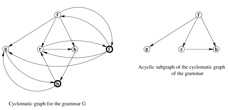
Figure 7: FVS–transformation.

Our widening operator for the analysis of equality relationships is defined in the following way. A vertex set of the cyclomatic graph of the grammar G is a set of functional symbols existing in G. An arc $(f,g)$ belongs to its arc set if G contains rules $A\rightarrow f(\ldots,B,\ldots)$ and $B\rightarrow g(\ldots)$. A transformation of a cyclomatic graph which involves detecting some FVS (it can be an upper approximation of a minimal feedback set) and removing all vertices from the FVS is said to be an FVS–transformation (an example is shown in Figure 7). Let $L\backslash_{\mbox{\tiny\bf FVS}}$ be a language obtained from $L$ by FVS–transformation applied to the grammar generating $L$. We define

$$L(\mbox{\bf G}_{1})\mbox{$\hbox to0.0pt{$\displaystyle\mbox{\raisebox{4.73611pt}[0.0pt][0.0pt]{\hskip 0.5pt$\sim$}}$\hss}\bigtriangledown$}L(\mbox{\bf G}_{2})=\left\{\begin{array}[]{ll}\mbox{$L(\mbox{\bf G}_{1})\backslash_{\mbox{\tiny\bf FVS}}$}~{}\mbox{$\cap$}~{}L(\mbox{\bf G}_{2})&\mbox{~{}if~{}~{}}|\mbox{\bf G}_{2}|\geq|\mbox{\bf G}_{1}|>d,\\ L(\mbox{\bf G}_{1})~{}\mbox{$\cap$}~{}\mbox{$L(\mbox{\bf G}_{2})\backslash_{\mbox{\tiny\bf FVS}}$}&\mbox{~{}if~{}~{}}|\mbox{\bf G}_{1}|>|\mbox{\bf G}_{2}|>d,\\ L(\mbox{\bf G}_{1})~{}\mbox{$\cap$}~{}L(\mbox{\bf G}_{2})&\mbox{~{}otherwise,}\end{array}\right.$$

where $d$ is a user-defined parameter. It is reasonable to choose this parameter, depending on number of variables of analyzed programs, as a linear function with a small factor of proportionality. Notice that in this case the lengths of appearing chains linearly depend on number of variables living simultaneously.

3.2 Divergence of the analysis

Is the widening operator, being rather complex, really needed for the analysis of equality relationships? Are there programs which, being analyzed, generate infinite chains of semantic properties? It should be mentioned that constructing such program examples has been a problem for a long time. In [18] we stated our belief that their existence seems hardly probable. These attempts failed, because they concentrated on constructing an example with completely non-interpretable functional symbols, i.e. in the frame of the “pure” theory of program schemata.

As already noticed, we can widely vary the interpretability of the analysis algorithm. In order to construct an example, it will suffice to use the following rule of completion:

$$\mbox{if }(t_{1}=t_{2})=TRU\!E\in L\mbox{ then {\bf Co}}(L)=\mbox{$L\hbox to0.0pt{$\displaystyle\{$\hss}\hskip 2.7pt|t_{1}\equiv t_{2}\hbox to0.0pt{$\displaystyle|$\hss}\}$}.$$

We consider the following example:

… x:=f(y); if  f(x)=f(y)  then    while  y=f(g(y))  do      y:=g(y)   end end …         program scheme

… x:=sign(y); if  sign(x)=sign(y)  then    while  y=sign(abs(y))  do      y:=abs(y)   end end …        “real-world” program

The properties computed at the body entry belong to an infinite decreasing chain. On Figure 8 a state $L_{e}$ describes properties valid before cycle execution; states $L_{1}$ and $L_{2}$ describe properties at the entry of the cycle body for first and second iteration, respectively. It is easy to see that $L_{1}\mbox{$\cap$}L_{2}$ coincides with $L_{2}$ except in the equality relationships containing terms generated by $g^{*}$. Therefore every time we obtain the next state, the functional element $g^{*}$ is absent and the sub-net placed in the dashed box will repeat more and more times.

Figure 8: The case of divergence of the analysis.

To obtain a “real-world” program from this program scheme, we interpret the functional symbols in the following manner: $f\equiv sign$ and $g\equiv abs$. We would like to point out the following interesting property. Execution of this piece of code (i.e., its behavior determined with the standard semantics) diverges only for two values of y: 0 and 1. At the same time the analysis algorithm (i.e. execution of the piece of code under our nonstandard semantics) is always divergent on condition that a widening operator is not used and the assumption on interpretation mentioned above holds.

Is this program actually real-world? The reader should decide that by himself but we would like to underline the following. On the one hand, the interpretability of the analysis algorithm can be varied in wide ranges and, on the other, we are not able to prove formally the impossibility of such behavior of the analyzer under the considered interpretation. So, we can choose either a lean analysis using acyclic grammars only or another one using arbitrary grammars and some widening operator.

3.3 Complexity of the analysis

In [18] we pointed out the following upper bound on time for the algorithm of ERA: $O(nmG^{2}_{max})$, where $n$ is program size, $m$ is maximum of number of program variables existing at a time, and $G_{max}$ is maximum of sizes of grammars appearing in course of the analysis. Due to our construction of widening operator (namely, choice of the parameter $d$ linearly depended on $m$) we can assume that $G_{max}=O(m)$.

This bound can be deduced with help of Theorem 6 in [5]. The theorem states that for the recursive strategy of chaotic iteration maximum complexity is

$$h\cdot\sum_{c\in C}\delta(c)\hskip 28.45274pt\left(\leq h\cdot|C|\cdot|W|\right),\hbox to0.0pt{$\displaystyle\hskip 71.13188pt{\bf(**)}$\hss}$$

where $h$ is maximum length of increasing chains built by a widening operator, $C$ is set of control program points, $\delta(c)$ is depth of the control point $c$ in hierarchy of nested strongly connected components of the control flow graph containing $c$, and $W$ is set of vertices where a widening operator is applied during the analysis.

For well-structured programs we can assume that maximum depth of nested loops does not depend on program size and is bounded by some constant. By ${\bf(**)}$ we conclude that number of algorithm steps does not exceed $O(nm)$. Since time complexity of all operations used in the analysis are estimated by $G^{2}_{max}$ we obtain $O(nmG^{2}_{max})$ (or $O(nm^{3})$) upper bound. Notice that to improve the results of the analysis it is possible to use rich semantic completion and more precise FVS–algorithms that have more than quadratic time complexity.

However, experimental results show that an approximation of a fixed point for the heads of cycle bodies is usually attained after at most two iterations and time complexity of the analysis is proportional to $nG_{max}$. Also, the user can turn off checking a threshold after which widening is started. In this case, he (consciously) admits some chance that the analysis diverges but we believe that this chance is not too big.

It is easy to see that the space complexity of the equality relationship analysis is $O(nG_{max})$ and it is essentially depended on the number of variables. We estimate the actual space requirements as 1.5–2.0 Mb per 1000 program lines for middle-size programs.

4 Processing of invariants and experimental results

4.1 Usage of ERA–invariants

ERA produces some set of invariants involving program terms which can be useful at different steps of program development and processing: debugging, verification (for that the invariants are interesting themselves), specialization, and optimization. The automatic prover mentioned above can be used at step of post-processing results of the analysis.

We notice that the analyzer can tell the user useful information both at the stage of analyzing (this means that it is possible that there exist execution traces where such computational states appear; we mark with $+$ properties which can be detected at this stage) and at the stage of processing of results of the analysis (these properties hold for each execution trace leading to this program point). We shall briefly list some program properties that can be extracted from computation states $L_{in}$ and $L_{out}$ being for a statement S the input and output states respectively.

$+$

Variable $x$ has an indefinite value if $L_{in}$ contains $x=\omega$.

$+$

Error in evaluation of an expression: division by zero, out of type ranges, nil–pointer dereferencing, etc.

$-$

S is inaccessible if $L_{in}=\mbox{$\top^{\prime}$}$. This information can correspond to different properties of program execution: potentially infinite cycles and recursive calls, dead branches of conditional statements, useless procedural definitions, etc.

$-$

Assignment statement v:=exp is redundant if $L_{out}$ contains $v=v^{\prime}$ where $v^{\prime}$ is the variable associated with $v$.

$-$

Unused definitions (constants, variables, types).

$-$

Constant propagation. Notice that ERA can detect that an expression is constant not only when constants for all variables in this expression are known.

$-$

More general: for some expression there exists an expression that is equal to the original one and calculated more efficiently (with respect to an given criterion time/space and target computer architecture).

Obviously, this list is not complete and there are many other properties which can be extracted from the invariants. For example, we can consider systems of equations/inequalities contained in the gathered invariants and try to solve them to derive more precise ranges for values of expressions or the inconsistency of this computational state.

Apart from the automatic mode when invariants are processed automatically, we provide an interactive mode to visualize results of our analysis in a hypertext system. HyperCode presented in [7, 3] is an open tunable system for visualization of properties of syntactic structures. There are two cases: visualization of all properties detected in the automatic mode and the user-driven processing and visualization of properties.

The experiments show that not all program properties of interest can be automatically extracted out of the computed invariants. It is not judicious to consider many particular cases and to hardly embed them into the system. Instead, the system facilitates the specification of the user request with some friendly interface. He chooses a program point and an expression and obtains those and only those equality relationships, valid at this point, where this expression occurs as a super- or sub-term.

4.2 Program examples

An example of a program is presented below. The properties detected by the analyzer are indicated in comments.

var x,y,z: integer;
procedure P(a,b: integer):integer;
begin	(*parameters are always equal*)
return a+b	(*expression can be simplified: 2*a*)
end P;
begin
Read(x);
while  x$\leq$0  do
Read(x);
x := x+1;
z := x+z;	(*variable z might be uninitialized*)
y := x+1;
if  x=0  then
z := y;	(*r-value can be simplified: z:=1*)
else
z := x+1;	(*r-value can be simplified: z:=y*)
x := y;
end;
Write( P(y,z) )	(*call can be transformed: Write(2*y)*)
end;
x := z div (y - z);	(*arithmetical error*)
Write(x)	(*inaccessible point*)
end.

On basis of the analysis, this program can be transformed into the following:

var x:integer;

begin

Read(x);

while  x$\leq$0  do

Read(x);   x := x+2;   Write(2*x)

end

ERROR_EXCEPTION;

end.

program	length (lines)			size (bytes)
	M2Mix	ERA	improv.	M2Mix	ERA	improv.
KMP	167	133	20.35%	2996	2205	26.4%
Lambert	361	326	9.7%	6036	2564	57.5%
Automaton	37	35	5.4%	969	926	4.5%
IntFib	87	77	11.5%	1647	1432	13.05%
Ackerman	64	62	3.1%	1384	1322	4.5%
	average		10.01%	average		21.19%

Table 2: Comparison ERA and M2Mix.

In Table 2 we present some results of optimization based on our analysis of residual programs generated by M2Mix specializer [6, 33]. To compile these examples, we used XDS Modula/Oberon compiler v.2.30 [20]. The following programs have been investigated:

• KMP — the “naïve” matching algorithm specialized with respect to some pattern; the residual program is comparable to Knuth, Morris, and Pratt’s algorithm in efficiency. (see also Appendix).

• Lambert — a program drawing Lambert’s figure and specialized with respect to number of points.

• Automaton — an interpreter of a deterministic finite-state automaton specialized with respect to some language.

• Int_Fib — an interpreter of MixLan [33] specialized with respect to a program computing Fibonacci numbers.

• Ackerman — a program computing some values of Akcerman’s function and specialized with respect to its first argument.

Let us comment briefly on the obtained results. Reducing length of a program can be considered as reducing number of operators and declarations. In these examples the optimizing effect was typically attained by the removal of redundant assignments, dead operators, unused variables and the reduction of operator strength. The only exception is KMP program characterized by high degree of polyvariance (roughly speaking it means presence of deep–nested conditional statements) and an active usage of array references. Here some IF–statements with constant conditions and redundant range checks were eliminated. Notice that the last optimizing transformation is very important for Modula–like languages where such checks are defined by the language standard. Such notable optimizing effect for the Lambert program is explained by deep reduction of power of floating-point operations which cannot be achieved by optimizing techniques now used in compilers. Since Automaton and Ackerman programs are quite small, their optimization gives conservative results. However, they would be better for the Ackerman program if the implementation of ERA were context-sensitive. Substantial speed-up of these optimized programs was not obtained (it was less than 2%) and this is not surprising since the great bulk of specializers take it as a criterion of optimality.

These experiments show that an average reduction of size of residual programs is 20–25%. Because the case of KMP program seems to be the most realistic, we suppose that such improvement can be achieved in practice for real–world programs and it will be increased for large residual programs with a high degree of polyvariance and active usage of arrays and float-point arithmetics. It is the author opinion that the analysis of automatically generated (from high–level specifications as well) programs is the most promising direction of its application, especially in the context-sensitive implementation of ERA.

Appendix. Analysis of KMP

The appendix presents results of application of ERA to KMP program generated by the specializer M2Mix. This program is a specialization of a program implementing the naïve pattern matching Match(p,str) with respect to the pattern p=”ababb”. The invariants are written as comments at program points where they hold. We can conclude that:

• The target string necessarily ends with ”#” and the variable ls is equal to the string length (line 10).

• Every time when some element of str (lines 20, 31, 42, 53, 58, 67, 72, 78, 86, 108, 113, 129, 140, 151, 162) is used in second LOOP, the value of its index expression does not exceed the value of the variable ls. The same is true for the value of a variable before the increment statements INC(s) (lines 23, 34, 45, 62, 81, 89, 94, 98, 103, 116, 120, 132, 143, 154, 165). Therefore, it suffices to check that a value of ls is not beyond the ranges determined by the type _TYPE354a04 during input of the target string (line 8). So, in the second cycle all range checks can be eliminated.

• The assignment _cfg_counter:=0 is redundant (line 24).

• Conditions str[s+2]=’a’ and str[s]=’a’ are always false (lines 78 and 86, respectively) because two different constants are equal. So, the code of THEN–branches is dead.

• The conditions at the lines 63, 68, 74, 82, 104, 109 are false, too. However, automatic detection of these properties are not as easily as the previous.

Using this semantic information, it is possible to build a new program functionally equivalent to Match(”ababb”,str). In text of the program given below the underlined code can be eliminated.

MODULE Match;
FROM FIO IMPORT File,Open,ReadChar,WriteInt,stdout;
VAR _cfg_counter : CARDINAL; str_file : File;
TYPE _TYPE354a04 = [0..20];
TYPE _TYPE355004 = ARRAY _TYPE354a04 OF CHAR;
VAR str : _TYPE355004; ls,s : _TYPE354a04;
BEGIN
1:     str_file := Open(”target.dat”);
2:     ls := 0;
3:     LOOP
4:          str[ls] := ReadChar(str_file);
5:          IF (str[ls]=’#’) THEN	$(*str[ls]=^{\prime}\!\!\#^{\prime}*)$
6:               EXIT
7:          ELSE	$(*str[ls]\neq^{\prime}\!\!\#^{\prime}*)$
8:               INC(ls)
9:          END
10:     END;	$(*str[ls]=^{\prime}\!\!\#^{\prime}*)$
11:     s := 0;
12:     _cfg_counter := 0;	$(*s=\_cfg\_counter=0*)$

13:     LOOP
14:          CASE _cfg_counter OF
15:          $|$ 0 :	$(*\_cfg\_counter=0*)$
16:               IF ((s+0)$\geq$ls) THEN	$(*s\geq ls*)$
17:                    WriteInt(stdout,(-1),0);
18:                    EXIT
19:               END;	$(*0<ls,s<ls*)$
20:               IF (str[(s+0)]=’a’) THEN	$(*str[s]=^{\prime}\!\!a^{\prime},0<ls,s<ls*)$
21:                    _cfg_counter := 1
22:               ELSE	$(*0<ls,s<ls,str[0]\neq^{\prime}\!\!a^{\prime}*)$
23:                    INC(s);	$(*\_cfg\_counter=0*)$
24:                    _cfg_counter := 0
25:               END	$(*0<ls,s<ls*)$
26:          $|$ 1 :	$(*\_cfg\_counter=1*)$
27:               IF ((s+1)$\geq$ls) THEN	$(*s+1\geq ls*)$
28:                    WriteInt(stdout,(-1),0);
29:                    EXIT
30:               END;	$(*s+1<ls*)$
31:               IF (str[(s+1)]=’b’) THEN	$(*str[s+1]=^{\prime}\!\!b^{\prime}*)$
32:                    _cfg_counter := 2
33:               ELSE	$(*str[s+1]\neq^{\prime}\!\!b^{\prime}*)$
34:                    INC(s);	$(*str[s]\neq^{\prime}\!\!b^{\prime},s<ls*)$
35:                    _cfg_counter := 0
36:               END
37:          $|$ 2 :	$(*\_cfg\_counter=2*)$
38:               IF ((s+2)$\geq$ls) THEN	$(*s+2\geq ls*)$
39:                    WriteInt(stdout,(-1),0);
40:                    EXIT
41:               END;	$(*s+2<ls*)$
42:               IF (str[(s+2)]=’a’) THEN	$(*str[s+2]=^{\prime}\!\!a^{\prime}*)$
43:                    _cfg_counter := 3
44:               ELSE	$(*str[s+2]\neq^{\prime}\!\!a^{\prime}*)$
45:                    INC(s);	$(*str[s+1]\neq^{\prime}\!\!a^{\prime},s+1<ls*)$
46:                    _cfg_counter := 4
47:               END
48:          $|$ 3 :	$(*\_cfg\_counter=3*)$
49:               IF ((s+3)$\geq$ls) THEN	$(*s+3\geq ls*)$
50:                    WriteInt(stdout,(-1),0);
51:                    EXIT
52:               END;	$(*s+3<ls*)$
53:               IF (str[(s+3)]=’b’) THEN	$(*str[s+3]=^{\prime}\!\!b^{\prime}*)$
54:                    IF ((s+4)$\geq$ls) THEN	$(*s+4\geq ls,s+3<ls*)$
55:                         WriteInt(stdout,(-1),0);
56:                         EXIT
57:                    END;	$(*s+4<ls*)$
58:                    IF (str[(s+4)]=’b’) THEN	$(*str[s+3]=str[s+4]=^{\prime}\!\!b^{\prime}*)$
59:                         WriteInt(stdout,s,0);
60:                         EXIT
61:                    ELSE	$(*str[s+3]=^{\prime}\!\!b^{\prime},str[s+4]\neq^{\prime}\!\!b^{\prime},s+4<ls*)$
62:                         INC(s);	$(*str[s+2]=^{\prime}\!\!b^{\prime},str[s+3]\neq^{\prime}\!\!b^{\prime},s+3<ls*)$
63:                         IF ((s+0)$\geq$ls) THEN	$(*s\geq ls,s+3<ls*)$
64:                              WriteInt(stdout,(-1),0);
65:                              EXIT
66:                         END;	$(*str[s+2]=^{\prime}\!\!b^{\prime},str[s+3]\neq^{\prime}\!\!b^{\prime},s+3<ls*)$
67:                         IF (str[(s+0)]=’a’) THEN	$(*str[s]=^{\prime}\!\!a^{\prime},str[s+2]=^{\prime}\!\!b^{\prime},str[s+3]\neq^{\prime}\!\!b^{\prime},$
	$\hskip 8.88892pts+3<ls*)$
68:                              IF ((s+1)$\geq$ls) THEN	$(*s+1\geq ls,s+3<ls*)$
69:                                   WriteInt(stdout,(-1),0);
70:                                   EXIT
71:                              END;	$(*\mbox{the same as at line 67}*)$

72:                              IF (str[(s+1)]=’b’) THEN	$(*str[s]=^{\prime}\!\!a^{\prime},str[s+1]=^{\prime}\!\!b^{\prime},str[s+2]=^{\prime}\!\!b^{\prime},$
73:	$\hskip 8.88892ptstr[s+3]\neq^{\prime}\!\!b^{\prime},s+3<ls*)$
74:                                   IF ((s+2)$\geq$ls) THEN	$(*s+2\geq ls,s+3<ls*)$
75:                                        WriteInt(stdout,(-1),0);
76:                                        EXIT
77:                                   END;	$(*str[s]=^{\prime}\!\!a^{\prime},str[s+1]=^{\prime}\!\!b^{\prime},str[s+2]=^{\prime}\!\!b^{\prime},$
	$\hskip 8.88892ptstr[s+3]\neq^{\prime}\!\!b^{\prime},s+3<ls*)$
78:                                   IF (str[(s+2)]=’a’) THEN	$(*\mbox{inaccessible point}*)$
79:                                        _cfg_counter := 3
80:                                   ELSE	$(*str[s]=^{\prime}\!\!a^{\prime},str[s+1]=^{\prime}\!\!b^{\prime},str[s+2]=^{\prime}\!\!b^{\prime},$
	$\hskip 8.88892ptstr[s+3]\neq^{\prime}\!\!b^{\prime},s+3<ls*)$
81:                                        INC(s);	$(*str[s-1]=^{\prime}\!\!a^{\prime},str[s]=^{\prime}\!\!b^{\prime},str[s+1]=^{\prime}\!\!b^{\prime},$
	$\hskip 8.88892ptstr[s+2]\neq^{\prime}\!\!b^{\prime},s+2<ls*)$
82:                                        IF ((s+0)$\geq$ls) THEN	$(*s\geq ls,s+2<ls*)$
83:                                             WriteInt(stdout,(-1),0);
84:                                             EXIT
85:                                        END;	$(*str[s-1]=^{\prime}\!\!a^{\prime},str[s]=^{\prime}\!\!b^{\prime},str[s+1]=^{\prime}\!\!b^{\prime},$
	$\hskip 8.88892ptstr[s+2]\neq^{\prime}\!\!b^{\prime},s+2<ls*)$
86:                                        IF (str[(s+0)]=’a’) THEN	$(*\mbox{inaccessible point}*)$
87:                                             _cfg_counter:=14
88:                                        ELSE	$(*str[s-1]=^{\prime}\!\!a^{\prime},str[s]=^{\prime}\!\!b^{\prime},str[s+1]=^{\prime}\!\!b^{\prime},$
	$\hskip 8.88892ptstr[s+2]\neq^{\prime}\!\!b^{\prime},s+2<ls*)$
89:                                             INC(s);	$(*str[s-2]=^{\prime}\!\!a^{\prime},str[s-1]=^{\prime}\!\!b^{\prime},str[s]=^{\prime}\!\!b^{\prime},$
	$\hskip 8.88892ptstr[s+1]\neq^{\prime}\!\!b^{\prime},s+1<ls*)$
90:                                             _cfg_counter:=4
91:                                        END
92:                                   END	$(*str[s-2]=^{\prime}\!\!a^{\prime},str[s-1]=^{\prime}\!\!b^{\prime},str[s]=^{\prime}\!\!b^{\prime},$
	$\hskip 8.88892ptstr[s+1]\neq^{\prime}\!\!b^{\prime},s+1<ls*)$
93:                              ELSE	$(*str[s]=^{\prime}\!\!a^{\prime},str[s+1]\neq^{\prime}\!\!b^{\prime},str[s+2]=^{\prime}\!\!b^{\prime},$
	$\hskip 8.88892ptstr[s+3]\neq^{\prime}\!\!b^{\prime},s+3<ls*)$
94:                                   INC(s);	$(*str[s-1]=^{\prime}\!\!a^{\prime},str[s]\neq^{\prime}\!\!b^{\prime},str[s+1]=^{\prime}\!\!b^{\prime},$
	$\hskip 8.88892ptstr[s+2]\neq^{\prime}\!\!b^{\prime},s+2<ls*)$
95:                                   _cfg_counter := 12
96:                              END
97:                         ELSE	$(*str[s]=^{\prime}\!\!a^{\prime},str[s+2]=^{\prime}\!\!b^{\prime},str[s+3]\neq^{\prime}\!\!b^{\prime},$
	$\hskip 8.88892pts+3<ls*)$
98:                              INC(s);	$(*str[s-1]=^{\prime}\!\!a^{\prime},str[s+1]=^{\prime}\!\!b^{\prime},str[s+2]\neq^{\prime}\!\!b^{\prime},$
	$\hskip 8.88892pts+2<ls*)$
99:                              _cfg_counter := 12
100:                         END
101:                    END
102:               ELSE	$(*str[s+3]\neq^{\prime}\!\!b^{\prime},s+3<ls*)$
103:                    INC(s);	$(*str[s+2]\neq^{\prime}\!\!b^{\prime},s+2<ls*)$
104:                    IF ((s+0)$\geq$ls) THEN	$(*s\geq ls,s+2<ls*)$
105:                         WriteInt(stdout,(-1),0);
106:                         EXIT
107:                    END;	$(*str[s+2]\neq^{\prime}\!\!b^{\prime},s+2<ls*)$
108:                    IF (str[(s+0)]=’a’) THEN	$(*str[s]=^{\prime}\!\!a^{\prime},str[s+2]\neq^{\prime}\!\!b^{\prime},s+2<ls*)$
109:                         IF ((s+1)$\geq$ls) THEN	$(*s+1\geq ls,s+2<ls*)$
110:                              WriteInt(stdout,(-1),0);
111:                              EXIT
112:                         END;	$(*str[s]=^{\prime}\!\!a^{\prime},str[s+2]\neq^{\prime}\!\!b^{\prime},s+2<ls*)$

113:                         IF (str[(s+1)]=’b’) THEN	$(*str[s]=^{\prime}\!\!a^{\prime},str[s+1]=^{\prime}\!\!b^{\prime},str[s+2]\neq^{\prime}\!\!b^{\prime},$
	$\hskip 8.88892pts+2<ls*)$
114:                              _cfg_counter := 2
115:                         ELSE	$(*str[s]=^{\prime}\!\!a^{\prime},str[s+2]\neq^{\prime}\!\!b^{\prime},s+2<ls*)$
116:                              INC(s);	$(*str[s-1]=^{\prime}\!\!a^{\prime},str[s+1]\neq^{\prime}\!\!b^{\prime},s+1<ls*)$
117:                              _cfg_counter := 10
118:                         END
119:                    ELSE	$(*str[s+2]\neq^{\prime}\!\!b^{\prime},s+2<ls*)$
120:                         INC(s);	$(*str[s+1]\neq^{\prime}\!\!b^{\prime},s+1<ls*)$
121:                         _cfg_counter := 10
122:                    END
123:               END
124:          $|$ 4 :	$(*\_cfg\_counter=4*)$
125:               IF ((s+0)$\geq$ls) THEN	$(*s\geq ls*)$
126:                    WriteInt(stdout,(-1),0);
127:                    EXIT
128:               END;	$(*s<ls*)$
129:               IF (str[(s+0)]=’a’) THEN	$(*str[s]=^{\prime}\!\!a^{\prime},s<ls*)$
130:                    _cfg_counter := 1
131:               ELSE	$(*str[s]\neq^{\prime}\!\!a^{\prime},s<ls*)$
132:                    INC(s);	$(*str[s-1]\neq^{\prime}\!\!a^{\prime},s\leq ls*)$
133:                    _cfg_counter := 0
134:               END
135:          $|$ 10:	$(*\_cfg\_counter=10*)$
136:               IF ((s+0)$\geq$ls) THEN	$(*s\geq ls*)$
137:                    WriteInt(stdout,(-1),0);
138:                    EXIT
139:               END;	$(*s<ls*)$
140:               IF (str[(s+0)]=’a’) THEN	$(*str[s]=^{\prime}\!\!a^{\prime},s<ls*)$
141:                    _cfg_counter := 1
142:               ELSE	$(*str[s]\neq^{\prime}\!\!a^{\prime},s<ls*)$
143:                    INC(s);	$(*str[s-1]\neq^{\prime}\!\!a^{\prime},s\leq ls*)$
144:                    _cfg_counter := 0
145:               END
146:          $|$ 12:	$(*\_cfg\_counter=12*)$
147:               IF ((s+0)$\geq$ls) THEN	$(*s\geq ls*)$
148:                    WriteInt(stdout,(-1),0);
149:                    EXIT
150:               END;	$(*s<ls*)$
151:               IF (str[(s+0)]=’a’) THEN	$(*str[s]=^{\prime}\!\!a^{\prime},s<ls*)$
152:                    _cfg_counter := 14
153:               ELSE	$(*str[s]\neq^{\prime}\!\!a^{\prime},s<ls*)$
154:                    INC(s);	$(*str[s-1]\neq^{\prime}\!\!a^{\prime},s\leq ls*)$
155:                    _cfg_counter := 4
156:               END
157:          $|$ 14:	$(*\_cfg\_counter=14*)$
158:               IF ((s+1)$\geq$ls) THEN	$(*s+1\geq ls*)$
159:                    WriteInt(stdout,(-1),0);
160:                    EXIT
161:               END;	$(*s+1<ls*)$
162:               IF (str[(s+1)]=’b’) THEN	$(*str[s+1]=^{\prime}\!\!b^{\prime},s+1<ls*)$
163:                    _cfg_counter := 2
164:               ELSE	$(*str[s+1]\neq^{\prime}\!\!b^{\prime},s+1<ls*)$
165:                    INC(s);	$(*str[s]\neq^{\prime}\!\!b^{\prime},s<ls*)$
166:                    _cfg_counter := 4
167:               END
168:          END
END
END Match.

References

- [1] A. Aho and J. Ullman. The theory of parsing, translation and compilation, volume 1. Prentice-Hall Inc., 1972.
- [2] B. Alpern, M.N. Wegman, and F.K. Zadeck. Detecting equality of variables in programs. In Proc. of the 15th Annual ACM Symposium Principles of Programming Languages, pages 1–11. ACM Press, 1988.
- [3] D. Baburin, M. Bulyonkov, P. Emelianov, and N. Filatkina. Visualization facilities in program reengineering. Programmirovanie, 27(2):21–33, 2001.
- [4] L. Berman and G. Markowsky. Linear and non-linear approximate invariants. Research Report RC7241, T.J. Watson Research Center of IBM, Yorktown, NY, 1976.
- [5] F. Bourdoncle. Efficient chaotic iteration strategies with widenings. In Proc. of the International Conference on Formal Methods in Programming and Their Applications, volume 735 of Lecture Notes in Computer Science, pages 129–141. Springer-Verlag, 1993.
- [6] M. Bulyonkov and D. Kochetov. Practical aspects of specialization of Algol-like programs. In Proc. of the International Seminar on Partial Evaluation, volume 1110 of Lecture Notes in Computer Science, pages 17–32. Springer-Verlag, 1996.
- [7] M. Bulyonkov and D. Kochetov. Visualization of program properties. Research Report 51, Institute of Informatics Systems, Novosibirsk, Russia, 1998.
- [8] R. Clarisó and J. Cortadella. The octahedron abstract domain. In Proc. of the 11th International Static Analysis Symposium, volume 3148 of Lecture Notes in Computer Science, pages 312–327. Springer–Verlag, 2004.
- [9] P. Cousot and R. Cousot. Abstract interpretation: A unified lattice model for static analysis of programs by construction or approximation of fixpoints. In Rec. of the 4th ACM Symposium on Principles of Programming Languages, pages 238–252. ACM Press, 1977.
- [10] P. Cousot and R. Cousot. Abstract interpretation and application to logic program. Journal of Logic Programming, 13(2–3):103–180, 1992.
- [11] P. Cousot and R. Cousot. Abstract interpretation frameworks. Journal of Logic and Computation, 2(4):511–547, 1992.
- [12] P. Cousot and R. Cousot. Formal languages, grammar and set–constraint–based program analysis by abstract interpretation. In Rec. of the Conference on Functional Programming Languages and Computer Architecture, pages 170–181. ACM Press, 1995.
- [13] P. Cousot and R. Cousot. Software analysis and model checking. In Proceedings of the 14th International Conference on Computer Aided Verification, volume 2404 of Lecture Notes in Computer Science, pages 37–56. Springer-Verlag, 2002.
- [14] P. Cousot and N. Halbwachs. Automatic discovery of linear restraints among variables of a program. In Records of the 5th annual ACM Symposium on Principles of Programming Languages, pages 84–96. ACM, ACM Press, January 1978.
- [15] A. Deutsch. Interprocedural may–alias analysis for pointers: beyond -limiting. SIGPLAN Notices, 29(6):230–241, 1994. Proc. of the ACM SIGPLAN’94 Conference on Program Language Design and Implementation.
- [16] P.G. Emelianov and D.E. Baburin. Semantic analyzer of Modula-programs. In Proc. of the 4th International Static Analysis Symposium, volume 1302 of Lecture Notes in Computer Science, pages 361–363. Springer–Verlag, 1997.
- [17] P.G. Emelianov and V.K. Sabelfeld. Analyzer of semantic properties of Modula-programms. In Software intellectualization and quality, pages 100–107. Institute of Informatics Systems, Novosibirsk, Russia, 1994.
- [18] P.G. Emelianov. Analysis of the equality relation for the program terms. In Proc. of the Third International Static Analysis Symposium, volume 1145 of Lecture Notes in Computer Science, pages 174–188. Springer–Verlag, 1996.
- [19] G. Even, J. Naor, B. Schieber, and M. Sudan. Approximating minimum feedback sets and multi-cuts. In Proc. of the 4th International Conference on Integer Programming and Combinatorial Optimization, volume 920 of Lecture Notes in Computer Science, pages 14–28. Springer–Verlag, 1995.
- [20] Excelsior LLC. Native xds-x86 modula-2/oberon-2 development toolset.
- [21] K. Gargi. A sparse algorithm for predicated global value numbering. In Proceedings of the ACM SIGPLAN 2002 Conference on Programming Language Design and Implementation, pages 45–56, 2002.
- [22] A.D. Gordon and A.M. Pitts, editors. High Order Operational Techniques in Semantics. Publications of Newton Institute. Cambridge University Press, 1998.
- [23] Ph. Granger. Static analysis of arithmetical congruences. International Journal of Computer Mathematics, 30:165–199, 1989.
- [24] Ph. Granger. Static analysis of linear congruence equalities among variables of a program. In Proceedings of the International Joint Conference on Theory and Practice of Software Developement, volume 493 of Lecture Notes in Computer Science, pages 169–192. Springer–Verlag, 1991.
- [25] S. Gulwani and G.C. Necula. Discovering affine equalities using random interpretation. In Proc. of the ACM SIGPLAN-SIGACT 2003 Principles of Programming Languages, pages 74–84, 2003.
- [26] S. Gulwani and G.C. Necula. A polynomial-time algorithm for global value numbering. In Proc. of the 11th International Static Analysis Symposium, volume 3148 of Lecture Notes in Computer Science, pages 212–227. Springer–Verlag, 2004.
- [27] N. Halbwachs, Y.-E. Proy, and P. Roumanoff. Verification of real-time systems using linear relation analysis. Formal Methods in System Design, 11(2):157–185, 1997.
- [28] Nevin Heintze, Joxan Jaffar, and Răzvan Voicu. A framework for combining analysis and verification. In Records of the 27th Annual ACM Symposium on Principles of Programming Languages, pages 26–39, 2000.
- [29] N. Heintze and J. Jaffar. Set constraint and set–based program analysis. In A. Borning, editor, Principles and Practice of Constraint Programming, volume 874 of Lecture Notes in Computer Science, pages 281–298. Springer–Verlag, 1994.
- [30] N.D. Jones and S.S. Muchnick, editors. Program Flow Analysis: Theory and Applications. Prentice-Hall, 1981.
- [31] N.D. Jones. Flow analysis of lazy higher–order functional programs. In S. Abramsky and C. Hankin, editors, Abstract Interpretation of Declarative Languages, pages 103–122. Ellis Horwood, 1987.
- [32] M. Karr. Affine relationships among variables of a program. Acta Informatica, 6:133–151, 1976.
- [33] D.V. Kochetov. Effective specialization of Algol–like programs. Ph.D. Thesis, Institute of Informatics Systems, Novosibirsk, Russia, 1995.
- [34] F. Masdupuis. Array operations abstraction using semantic analysis of trapezoid congruences. In Proceedings of the International Conference on Supercomputing, pages 226–235. ACM Press, 1992.
- [35] F. Masdupuis. Semantic analysis of interval congruences. In Proceedings of the International Conference Formal Methods in Programming and Their Applications, volume 735 of Lecture Notes in Computer Science, pages 142–155. Springer–Verlag, 1993.
- [36] A. Miné. A new numerical abstract domain based on difference-bound matrices. In Proceedings of the Second Symposium on Programs as Data Objects, volume 2053, pages 155–169, 2001.
- [37] B.K. Rosen. Robust linear algorithms for cutsets. Journal Algorithms, 3:205–217, 1982.
- [38] O. Rüthing, J. Knoop, and B. Steffen. Detecting equalities of variables: Combining efficiency with precision. In Proc. of the 6th International Static Analysis Symposium, volume 1694 of Lecture Notes in Computer Science, pages 232–247. Springer–Verlag, 1999.
- [39] V. Sabelfeld. Polynomial upper bound for the complexity of the logic-termal equivalence decision. Doklady Akademii Nauk, Matematika, 249(4):793–796, 1979.
- [40] V. Sabelfeld. The logic–termal equivalence is polynomial–time decidable. Information Processing Letters, 10(2):102–112, 1980.
- [41] E. Speckenmeyer. On feedback problems in digraphs. In Proceedings of the 15th International Workshop on Graph–Theoretic Concepts in Computer Science, volume 411 of Lecture Notes in Computer Science, pages 218–231. Springer–Verlag, 1990.
- [42] A. Venet. Automatic analysis of pointer aliasing for untyped programs. Science of Computer Programming, 35(2-3):223–248, 1999.
- [43] M. Wegman and F.K. Zadeck. Constant propagation with conditional branches. ACM Transactions on Programming Language and Systems, 13(2):181–210, 1991.