Asymptotic Spectral Distribution of Crosscorrelation Matrix in Asynchronous CDMA

Abstract

Asymptotic spectral distribution (ASD) of the crosscorrelation matrix is investigated for a random spreading short/long-code asynchronous direct sequence-code division multiple access (DS-CDMA) system. The discrete-time decision statistics are obtained as the output samples of a bank of symbol matched filters of all users. The crosscorrelation matrix is studied when the number of symbols transmitted by each user tends to infinity. Two levels of asynchronism are considered. One is symbol-asynchronous but chip-synchronous, and the other is chip-asynchronous. The existence of a nonrandom ASD is proved by moment convergence theorem, where the focus is on the derivation of asymptotic eigenvalue moments (AEM) of the crosscorrelation matrix. A combinatorics approach based on noncrossing partition of set partition theory is adopted for AEM computation. The spectral efficiency and the minimum mean-square-error (MMSE) achievable by a linear receiver of asynchronous CDMA are plotted by AEM using a numerical method.

I Introduction

Direct sequence-code division multiple access (DS-CDMA) is one of the most flexible and commonly proposed multiple access techniques for wireless communication systems. To gain deeper insights into the performance of receivers in a CDMA system, much work has been devoted to the analysis of random spreading CDMA in the large-system regime, i.e., both the number of users $K$ and the number of chips $N$ per symbol approach infinity with their ratio $K/N$ kept as a finite positive constant $\beta$ [1, 2, 3]. Such asymptotic analysis of random spreading CDMA enables random matrix theory to enter communication and information theory. In the last few years, a considerable amount of CDMA research has made substantial use of results in random matrix theory (see [4] and references therein).

In this paper, we focus on the derivation of the asymptotic spectral distribution (ASD) of the crosscorrelation matrix in asynchronous CDMA systems. Consider the linear vector memoryless channels of the form $\boldsymbol{y}=\boldsymbol{H}\boldsymbol{x}+\boldsymbol{w}$, where $\boldsymbol{x}$, $\boldsymbol{y}$ and $\boldsymbol{w}$ are the input vector, output vector and additive white Gaussian noise (AWGN) vector, respectively, and $\boldsymbol{H}$ denotes the random channel matrix independent of $\boldsymbol{w}$. This linear model encompasses a variety of applications in communications such as multiuser channels, multi-antenna channels, multipath channels, and, in particular, asynchronous CDMA channels of our interest in this research, etc., with $\boldsymbol{x}$, $\boldsymbol{y}$ and $\boldsymbol{H}$ taking different meanings in each case. Concerned with the linear model, it is of particular interest to investigate the limiting distribution of eigenvalues of the random matrix $\boldsymbol{H}{\boldsymbol{H}}^{\dagger}$ or $\boldsymbol{H}^{\dagger}{\boldsymbol{H}}$, called the ASD of the random matrix, when the column and row sizes of ${\boldsymbol{H}}$ tend to infinity but the ratio of sizes is fixed as a finite constant. Since ASD is deterministic and irrelevant to realizations of random parameters, it is convenient to use the asymptotic limit as an approximation for finite-sized system design and analysis. Moreover, it is quite often that ASD provides us with much more insights than an empirical spectral distribution (ESD) does. Even though ASD is obtained with the large-system assumption, in practice, the system enjoys large-system properties for a moderate size of the channel matrix.

Some applications of ASD in communication and information theory are exemplified below. Take the linear model ${\boldsymbol{y}}={\boldsymbol{H}}{\boldsymbol{x}}+{\boldsymbol{w}}$ for illustration. A number of the system performance measures, e.g. channel capacity and the minimum mean-square-error (MMSE) achievable by a linear receiver, is determined by the ESD of the matrix ${\boldsymbol{H}}{\boldsymbol{H}}^{\dagger}$. The asymptotic capacity and MMSE obtained by using ASD as an approximation of ESD can often result in closed-form expressions [5, 2]. It is also shown in [6, 7, 8, 9] that empirical eigenvalue moments (or, more conveniently, AEM) can be used to find the optimal weights of the reduced-rank MMSE receivers and its output signal-to-interference-ratio (SIR) in a large system. Moreover, a functional related to AEM is defined as the free expectation of random matrices in free probability theory [10], which has been recently applied to the asymptotic random matrix analysis.

For synchronous DS-CDMA systems, it is well known that the ASD of the crosscorrelation matrix follows Marc̆enko-Pastur law [5]. Also, explicit expressions for the AEM under the environments of unfaded, frequency-flat fading with single and multiple antennas, and frequency-selective fading are derived in [11, 12]. Actually, most of the research results on random spreading CDMA making use of random matrix theory are confined to synchronous systems. Just a few of them investigate asynchronous systems [13, 14, 15, 16, 17, 18, 19]. The goal of this work is to find out the ASD of crosscorrelation matrix in asynchronous CDMA systems given a set of users’ relative delays and an arbitrary chip waveform. As the uplink of a CDMA system is asynchronous, this work is motivated by the needs to study the problem of asynchronous transmission that is important but much less explored in the area of random matrix theory.

Two levels of asynchronism are considered in this paper, i.e., symbol-asynchronous but chip-synchronous, and chip-asynchronous. In the sequel, chip-synchronous is used for short to denote the former, and symbol-synchronous represents an ideal synchronous system. To be more specific, the relative delays among users are integer multiples of the chip duration in chip-synchronous CDMA, while they are any real numbers in chip-asynchronous CDMA.

Some previous results on asynchronous CDMA are reviewed. In [13], it is shown that the output SIR of the linear MMSE receiver in chip-synchronous CDMA converges to a deterministic limit characterized by the solution of a fixed-point equation that depends on the received power and the relative delay distributions of the users. When the width of the observation window during detection tends to infinity, the limiting output SIR converges to that of a symbol-synchronous system having all identical parameters. The system model of [13] splits each interferer into two virtual users, which leads to a crosscorrelation matrix with neither independent nor identically distributed entries. Results of [13] are obtained by employing Stieltjes transform for random matrices of that type. In [16], some equivalence results about the MMSE receiver output are provided for CDMA systems with various synchronism levels. In specific, when the ideal Nyquist sinc pulse is adopted as the chip waveform of a chip-asynchronous system, the asymptotic SIR at the MMSE detector output is the same as that in an equivalent chip-synchronous system for any observation window width; moreover, as the observation window width increases, the output SIR in chip-asynchronous CDMA converges further to that in an equivalent symbol-synchronous system. In [18], the analysis of linear multiuser detectors is provided for a symbol quasi-synchronous but chip-asynchronous system, called symbol-quasi-synchronous for short. It is demonstrated that, when the bandwidth of the chip waveform is smaller than $1/(2T_{c})$, where $T_{c}$ is the chip duration, the performance of symbol-quasi-synchronous and symbol-synchronous systems coincides independently of the chip waveform and the distribution of relative delays among users, where the performance is characterized by the output SIR of a reduced-rank MMSE detector when a square-root raised cosine pulse is adopted as the chip waveform. If the bandwidth is larger than the threshold, the former system outperforms the latter. Actually, when the chip waveform bandwidth is narrower than the threshold, the inter-chip interference (ICI) free property is lost [20], which leads to a severe degradation in performance.

In this paper, the system model is constructed without the user splitting executed in [13]. In stead, sufficient statistics obtained in the same way as [21, 22, 23] are employed. We assume the width of the observation window for symbol detection tends to infinity. The formulas for AEM of the crosscorrelation matrix are derived using a combinatorics approach. In specific, we use noncrossing partition in set partition theory as the solving tool to exploit all nonvanishing terms in the expressions of AEM. The combinatorics approach has been adopted in [11, 24, 25, 26, 27, 28] to compute AEM of random matrices in symbol-synchronous systems. All of them, either explicitly or implicitly, make use of graphs to signify noncrossing partitions. In this work, a graphical representation of $K$-graph, which is able to simultaneously represent a noncrossing partition and its Kreweras complementation map [29], is adopted. This property of a $K$-graph facilitates the employment of noncrossing partition and free probability theory in solving problems of interest.

In some applications of probability theory, it is frequent that the (infinite) moment sequence of an unknown distribution is available, and these moments determine a unique distribution. Suppose that the goal is to calculate the expected value of a certain function $g$ of the random variable $X$ whose distribution is unknown. One of the most widely used techniques is based on the Gauss quadrature rule method [30], where the expected value of $g(X)$ is expressed as a linear combination of samples of $g(x)$, and moments of $X$ are used to determine the coefficients in the combination and the points to be sampled. In this paper, the Gauss quadrature rule method is employed to compute the spectral efficiency and MMSE of asynchronous CDMA using the derived AEM.

This paper is organized as follows. In Section II, the crosscorrelation matrices are given for chip-synchronous and chip-asynchronous CDMA systems. Some definitions regarding the limit of of a random matrix are also introduced. In Section III, we derive AEM and ASD of corsscorrelation matrices in both chip-synchronous and chip-asynchronous systems. In Section IV, free probability theory is employed to obtain the spectra of sum and product of crosscorrelation matrix and a random diagonal matrix. In Section V, mathematical results demonstrated in this paper are connected to some known results. Discussions of the spectral efficiency and MMSE in an asynchronous CDMA system are provided in Section VI. Finally, this paper is concluded in Section VII.

II Crosscorrelation Matrix of Asynchronous CDMA

Consider asynchronous direct sequence-code division multiple access (DS-CDMA) systems where each user’s spreading sequence is chosen randomly and independently. There are $K$ users in the system, and the number of chips in a symbol is equal to $N$. We focus on the uplink of the system and assume the receiver knows the spreading sequences and relative delays of all users. Systems with two levels of asynchronism are considered, i.e., symbol-asynchronous but chip-synchronous, and chip-asynchronous. In the sequel, chip-synchronous is used for short to denote the former, and symbol-synchronous refers to an ideal synchronous system. To differentiate notations of chip-synchronous and chip-asynchronous systems, subscripts in text form of ”cs” and ”ca” are used for notations in the former and the latter systems, respectively.

II-A Chip-Synchronous CDMA

Denote the relative delay of user $k$ as $\tau_{k}$. For convenience, users are labelled chronologically by their arrival time, and $\{\tau_{k}\}_{k=1}^{K}$ satisfy

$$0=\tau_{1}\leq\tau_{2}\leq\cdots\leq\tau_{K}<NT_{c},$$ (1)

where $T_{c}$ is the chip duration, and all $\tau_{k}$’s are integer multiples of $T_{c}$. Suppose that each user sends a sequence of symbols with indices from $-M$ to $M$. In the complex baseband notation, the contribution of user $l$ to the received signal in a frequency-flat fading channel is

$$x_{l}(t)=\sum_{n=-M}^{M}A_{l}(n)b_{l}(n)\sum_{q=nN}^{(n+1)N-1}c_{l}^{(q)}\psi(t-qT_{c}-\tau_{l}),$$

where $b_{l}(n)$ is the $n$-th symbol of user $l$, $A_{l}(n)$ is the complex amplitude at the time $b_{l}(n)$ is received, $\{c_{l}^{(q)}:nN\leq q\leq(n+1)N-1\}$ is the spreading sequence assigned to the $n$-th symbol of user $l$, and $\psi(t)$ is the normalized chip waveform having the zero ICI condition of

$$\int_{-\infty}^{\infty}\psi(t)\psi(t-rT_{c})\textrm{d}t=\left\{\begin{array}[]{ll}1,&r=0,\\ 0,&r\in\mathbb{Z}\setminus\{0\}.\end{array}\right.$$ (2)

It is assumed that $\{b_{l}(n)\}_{n=-M}^{M}$ is a collection of independent equiprobable $\pm 1$ random variables. The symbol streams of different users are independent. The distribution of a scaled chip $\sqrt{N}c_{l}^{(q)}$ has zero mean, unit variance and finite higher order moments. We do not assume a particular distribution of $c_{l}^{(q)}$. Two distinct spreading mechanisms are considered, i.e., short-code and long-code. In a short-code system, the spreading sequences are randomly chosen for the first symbols, i.e., $b_{k}(-M)$ for user $k$, and remain the same for every symbol. In a long-code system, the spreading sequences are randomly and independently picked from symbol to symbol. The sequences of received amplitudes $\{A_{k}(m)\}_{m=-M}^{M}$ and $\{A_{l}(n)\}_{n=-M}^{M}$ are independent if $k\neq l$.

The complex baseband received signal is given by

$$r(t)=\sum_{l=1}^{K}x_{l}(t)+w(t),$$ (3)

where $w(t)$ is the baseband complex Gaussian ambient noise with independent real and imaginary components. The correlation function of $w(t)$ is $\textrm{E}\{w(t)w(t+\tau)^{*}\}=N_{0}\delta_{D}(\tau)$ with $\delta_{D}(\tau)$ being the Dirac delta function. The symbol matched filter output of user $k$’s symbol $m$, denoted as $y_{k}(m)$, is obtained by correlating $r(t)$ with the signature waveform of user $k$’s symbol $m$

$$y_{k}(m) = \int_{-\infty}^{\infty}r(t)\left(\sum_{p=mN}^{(m+1)N-1}c_{k}^{(p)}\psi(t-pT_{c}-\tau_{k})\right)\textrm{d}t$$ (4)

$$= \sum_{l=1}^{K}\sum_{n=-M}^{M}A_{l}(n)b_{l}(n)\rho_{\textrm{cs}}(m,n;k,l)+v_{k}(m),$$ (5)

where $v_{k}(m)$ results from the ambient noise $w(t)$, and $\rho_{\textrm{cs}}(m,n;k,l)$ is the crosscorrelation of spreading sequences at user $k$’s $m$-th symbol and user $l$’s $n$-th symbol, given as

$$\sum_{q=nN}^{(n+1)N-1}\sum_{p=mN}^{(m+1)N-1}c_{l}^{(q)}c_{k}^{(p)}\int_{-\infty}^{\infty}\psi(t-qT_{c}-\tau_{l})\psi(t-pT_{c}-\tau_{k})\textrm{d}t.$$ (6)

Due to the zero ICI condition of (2), the integral in (6) is nonzero (equal to one) if and only if $pT_{c}+\tau_{k}=qT_{c}+\tau_{l}$. Thus, we obtain

$$\rho_{\textrm{cs}}(m,n;k,l)=\sum_{p=mN}^{(m+1)N-1}\sum_{q=nN}^{(n+1)N-1}c_{k}^{(p)}c_{l}^{(q)}\delta(pT_{c}+\tau_{k},qT_{c}+\tau_{l}),$$ (7)

with $\delta(i,j)$ the Kronecker delta function. Since $0\leq\tau_{k},\tau_{l}\leq(N-1)T_{c}$, for a specific symbol index $m$, the $\delta$ function in (7) is equal to zero if $n\notin\{m-1,m,m+1\}$. Thus, we rewrite (5) as

$$y_{k}(m)=\sum_{l=1}^{K}\sum_{n=\max\{m-1,-M\}}^{\min\{m+1,M\}}A_{l}(n)b_{l}(n)\rho_{\textrm{cs}}(m,n;k,l)+v_{k}(m),\qquad-M\leq m\leq M.$$ (8)

Define the symbol matched filter output vector at the $m$-th symbol as

$${\underline{y}}(m)=[y_{1}(m),y_{2}(m),\cdots,y_{K}(m)]^{T},$$

and let the transmitted symbol vector ${\underline{b}}(m)$ and the noise vector ${\underline{v}}(m)$ have the same structures as ${\underline{y}}(m)$. Moreover, we define a block matrix $\boldsymbol{R}_{\textrm{cs}}$ whose $(k,l)$-th element of the $(m,n)$-th block, with $-M\leq m,n\leq M$, $1\leq k,l\leq K$, is equal to $\rho_{\textrm{cs}}(m,n;k,l)$ in (7). The square bracket $[\cdot]$ is used to indicate a specific element of the matrix $\boldsymbol{R}_{\textrm{cs}}$. Specifically, $[\boldsymbol{R}_{\textrm{cs}}]_{mn,kl}$ represents the $(k,l)$-th entry of the $(m,n)$-th block of the block matrix $\boldsymbol{R}_{\textrm{cs}}$. When we just want to point out a specific block, only the first set of indices is used, i.e., $[\boldsymbol{R}_{\textrm{cs}}]_{mn}$.

Using the notations defined above, we can show from (8) that

$${\underline{y}}(m)=\sum_{n=\max\{m-1,-M\}}^{\min\{m+1,M\}}[\boldsymbol{R}_{\textrm{cs}}]_{mn}{\underline{A}}(n){\underline{b}}(n)+{\underline{v}}(m),$$

where ${\underline{A}}(n)=\operatorname{diag}\{A_{1}(n),A_{2}(n),$ $\cdots,A_{K}(n)\}$. Stacking up ${\underline{y}}(m)$’s to yield the symbol matched filter output of the whole transmission period as

$$\boldsymbol{y}=\left[{\underline{y}}^{T}(-M),{\underline{y}}^{T}(-M+1),\cdots,{\underline{y}}^{T}(M)\right]^{T},$$

we obtain the discrete-time signal model

$$\boldsymbol{y}=\boldsymbol{R}_{\textrm{cs}}\boldsymbol{A}\boldsymbol{b}+\boldsymbol{v},$$ (9)

where $\boldsymbol{b}$ and $\boldsymbol{v}$ have the same structures as $\boldsymbol{y}$, $\boldsymbol{A}=\operatorname{diag}\{{\underline{A}}(-M),{\underline{A}}(-M+1)\cdots,{\underline{A}}(M)\}$, and the block matrix $\boldsymbol{R}_{\textrm{cs}}$ has a tri-diagonal structure of

$$\left[\begin{array}[]{ccccccc}\ddots&\ddots&\ddots&&&&\\ &[\boldsymbol{R}_{\textrm{cs}}]_{-1\hskip 0.56905pt-2}&[\boldsymbol{R}_{\textrm{cs}}]_{-1\hskip 0.56905pt-1}&[\boldsymbol{R}_{\textrm{cs}}]_{-1\hskip 0.56905pt0}&&&\\ &&[\boldsymbol{R}_{\textrm{cs}}]_{0\hskip 0.56905pt-1}&[\boldsymbol{R}_{\textrm{cs}}]_{0\hskip 0.56905pt0}&[\boldsymbol{R}_{\textrm{cs}}]_{0\hskip 0.56905pt1}&&\\ &&&[\boldsymbol{R}_{\textrm{cs}}]_{1\hskip 0.56905pt0}&[\boldsymbol{R}_{\textrm{cs}}]_{1\hskip 0.56905pt1}&[\boldsymbol{R}_{\textrm{cs}}]_{1\hskip 0.56905pt2}&\\ &&&&\ddots&\ddots&\ddots\end{array}\right].$$ (10)

Since $\tau_{k}\leq\tau_{l}$ for $k<l$, $[\boldsymbol{R}_{\textrm{cs}}]_{m\hskip 2.84526ptm-1}$ and $[\boldsymbol{R}_{\textrm{cs}}]_{m\hskip 2.84526ptm+1}$ are strict (zero diagonal) upper- and lower-triangular matrices, respectively. From the signal model given in (9), $\boldsymbol{R}_{\textrm{cs}}$ can be viewed as the crosscorrelation matrix of chip-synchronous CDMA. It can be shown that the correlation matrix of the noise vector ${\boldsymbol{v}}$ in (9) is $\textrm{E}\{{\boldsymbol{v}}{\boldsymbol{v}}^{\dagger}\}=N_{0}{\boldsymbol{R}}_{\textrm{cs}}$. Let ${\boldsymbol{R}}_{\textrm{cs}}={\boldsymbol{H}}_{\textrm{cs}}{\boldsymbol{H}}_{\textrm{cs}}^{\dagger}$ be a decomposition of ${\boldsymbol{R}}_{\textrm{cs}}$. We can perform the whitening process by left-multiplying ${\boldsymbol{y}}$ in (9) with ${\boldsymbol{H}}_{\textrm{cs}}^{-1}$, resulting in

$${\boldsymbol{z}}={\boldsymbol{H}}_{\textrm{cs}}^{-1}{\boldsymbol{y}}={\boldsymbol{H}}_{\textrm{cs}}^{\dagger}{\boldsymbol{A}}{\boldsymbol{b}}+{\boldsymbol{w}},$$ (11)

where the noise vector ${\boldsymbol{w}}={\boldsymbol{H}}_{\textrm{cs}}^{-1}{\boldsymbol{v}}$ is white and has the correlation matrix $N_{0}{\boldsymbol{I}}$.

II-B Chip-Asynchronous CDMA

In chip-asynchronous CDMA, the assumption that $\tau_{k}$’s are integer multiples of the chip duration $T_{c}$ no longer exists. Although the relative delays of users are not integer multiples of $T_{c}$, it is assumed that the zero ICI condition still holds. Thus, the property of zero ICI exists for chips of each particular user. Similarly to (5), the symbol matched filter output $y_{k}(m)$ can be expressed as

$$y_{k}(m)=\sum_{l=1}^{K}\sum_{n=-M}^{M}A_{l}(n)b_{l}(n)\rho_{\textrm{ca}}(m,n;k,l)+v_{k}(m),$$ (12)

where $\rho_{\textrm{ca}}(m,n;k,l)$ is different from $\rho_{\textrm{cs}}(m,n;k,l)$ in (5) since the zero ICI condition does not hold when the time difference of chip waveforms is not integer multiples of $T_{c}$. At this moment, the crosscorrelation $\rho_{\textrm{ca}}(m,n;k,l)$ is given by

$$\rho_{\textrm{ca}}(m,n;k,l)=\sum_{p=mN}^{(m+1)N-1}\sum_{q=nN}^{(n+1)N-1}c_{k}^{(p)}c_{l}^{(q)}R_{\psi}((p-q)T_{c}+\tau_{k}-\tau_{l}),$$ (13)

where

$$R_{\psi}(x)=\int_{-\infty}^{\infty}\psi(t)\psi(t-x)\textrm{d}t$$ (14)

is the autocorrelation function of the chip waveform $\psi(t)$. We define the block matrix $\boldsymbol{R}_{\textrm{ca}}$ whose $(k,l)$-th component of the $(m,n)$-th block, with $-M\leq m,n\leq M$ and $1\leq k,l\leq K$, is equal to $\rho_{\textrm{ca}}(m,n;k,l)$ given in (13). It can be shown that

$${\underline{y}}(m)=\sum_{n=-M}^{M}[\boldsymbol{R}_{\textrm{ca}}]_{mn}{\underline{A}}(n){\underline{b}}(n)+{\underline{v}}(m),$$ (15)

and we obtain the discrete-time signal model

$$\boldsymbol{y}=\boldsymbol{R}_{\textrm{ca}}\boldsymbol{A}\boldsymbol{b}+\boldsymbol{v},$$ (16)

where $\boldsymbol{R}_{\textrm{ca}}$ is thus seen as the crosscorrelation matrix of a chip-asynchronous CDMA system. Note that, unlike the tri-diagonal structure of $\boldsymbol{R}_{\textrm{cs}}$ shown in (10), the matrix $\boldsymbol{R}_{\textrm{ca}}$ generally does not possess such structure except when the autocorrelation function $R_{\psi}(x)$ has a finite span. We can perform whitening on (16) to yield a linear model

$$\boldsymbol{z}=\boldsymbol{H}_{\textrm{ca}}^{\dagger}\boldsymbol{A}\boldsymbol{b}+\boldsymbol{w},$$ (17)

where ${\boldsymbol{R}}_{\textrm{ca}}=\boldsymbol{H}_{\textrm{ca}}\boldsymbol{H}_{\textrm{ca}}^{\dagger}$ and ${\boldsymbol{w}}=\boldsymbol{H}_{\textrm{ca}}^{-1}{\boldsymbol{v}}$ is a white noise vector.

The discrete statistics $\boldsymbol{y}$ in (9) and (16), and hence $\boldsymbol{z}$ in (11) and (17), for chip-synchronous and chip-asynchronous systems, respectively, are sufficient and are obtained in the same way as [21, 22, 23]. These sufficient statistics are the output samples of a bank of filters matched to the symbol spreading waveforms of all users. An alternative approach to generating statistics, adopted by [13, 31, 16, 15], is to pass the received signal to a chip matched filter and sample the output. Statistics yielded in this way are sufficient only under symbol- and chip-synchronous assumptions, and are not sufficient in the chip-asynchronous case. For a chip-asynchronous system, it is reported in [32] that, when the chip waveform is time limited to the chip interval, statistics obtained by sampling the chip matched filtering output at the chip rate leads to significant degradation in performance. On the other hand, if the output is sampled at up to the Nyquist rate, the loss in performance is negligible.

II-C Asymptotic Spectral Distribution of Crosscorrelation Matrix

The analysis of asynchronous CDMA systems will be conducted in a large system regime. That is, we assume both the number of users $K$ and the spreading gain $N$ approach infinity with their ratio $K/N$ converging to a non-negative constant $\beta$. To proceed the analysis, some definitions regarding the limit of a random matrix [33] are introduced. Let ${\boldsymbol{S}}^{(p)}$ denote a $p\times p$ Hermitian random matrix whose each element is a random variable. Suppose that ${\boldsymbol{S}}^{(p)}$ has eigenvalues $\nu_{1}\leq\nu_{2}\leq\cdots\leq\nu_{p}$. Since ${\boldsymbol{S}}^{(p)}$ is Hermitian, all $\nu_{i}$’s are real. The ESD of ${\boldsymbol{S}}^{(p)}$ is defined as

$$F^{(p)}(x)=p^{-1}\#\{i:\nu_{i}\leq x\},$$ (18)

where $\#\{\cdots\}$ denotes the number of elements in the indicated set. A simple fact is the $n$-th moment of $F^{(p)}(x)$ can be represented as

$$m_{n}^{(p)}=\int_{-\infty}^{\infty}x^{n}\textrm{d}F^{(p)}(x)=p^{-1}\operatorname{tr}(({\boldsymbol{S}}^{(p)})^{n}),$$ (19)

where tr is the trace operator, and the second equality holds because $\operatorname{tr}(({\boldsymbol{S}}^{(p)})^{n})=\sum_{i=1}^{p}\nu_{i}^{n}$. If $F^{(p)}(x)$ converges to a nonrandom function $F(x)$ as $p\rightarrow\infty$, then we say that the sequence $\{{\boldsymbol{S}}^{(p)}:p=1,2,\cdots\}$ has an ASD $F(x)$. To show that $F^{(p)}(x)$ tends to a limit, the moment convergence theorem [34] can be employed. To be specific, the theorem is stated here in a form convenient for this paper.

Theorem 1

[Moment Convergence Theorem] Let $\{F^{(p)}(x):p=1,2,\cdots\}$ be a sequence of distribution for which the moments

$$m_{n}^{(p)}=\int_{-\infty}^{\infty}x^{n}\textrm{d}F^{(p)}(x)$$

exist for all $n=0,1,2,\cdots$. Furthermore, let $F(x)$ be a distribution function for which the moments

$$m_{n}=\int_{-\infty}^{\infty}x^{n}\textrm{d}F(x)$$ (20)

exist for all $n=0,1,2,\cdots$. If

$$\lim_{p\rightarrow\infty}m_{n}^{(p)}=m_{n}$$ (21)

for all $n=0,1,2,\cdots$ in some sense, and if $F(x)$ is uniquely determined by the sequence of moments $m_{0},m_{1},m_{2},\cdots$, then

$$\lim_{p\rightarrow\infty}F^{(p)}(x)=F(x),$$

and the convergence holds in the same sense as that of (21). $\blacksquare$

The moment convergence theorem has a long history. The details can be found in [35]. In applying this theorem to show the existence of the ASD $F(x)$, we should determine the asymptotic moment sequence $\{m_{n}\}$ in (20) and prove that a unique distribution is determined by $\{m_{n}\}$. In [36], Carleman gave a sufficient condition $\sum_{n=1}^{\infty}m_{2n}^{-1/(2n)}=\infty$, called Carleman’s criterion, for the uniqueness of a distribution given a moment sequence $\{m_{n}\}$.

Concerned with the linear models of (11) and (17), it is of interest to consider the ESD of the random matrix ${\boldsymbol{H}}^{\dagger}_{\textrm{x}}{\boldsymbol{A}}({\boldsymbol{H}}^{\dagger}_{\textrm{x}}{\boldsymbol{A}})^{\dagger}$, $\textrm{x}\in\{\textrm{cs},\textrm{ca}\}$ [4, Chapter 1]. Represent matrices ${\boldsymbol{H}}_{\textrm{x}}$, ${\boldsymbol{A}}$, and ${\boldsymbol{R}}_{\textrm{x}}$ by ${\boldsymbol{H}}_{\textrm{x}}^{(K)}$, ${\boldsymbol{A}}^{(K)}$, and ${\boldsymbol{R}}_{\textrm{x}}^{(K)}$, respectively, when the user size of the system is $K$. In order to use Theorem 1 to find the ASD of the random matrix ${{\boldsymbol{H}}_{\textrm{x}}^{(K)}}^{\dagger}{\boldsymbol{A}}^{(K)}{{\boldsymbol{A}}^{(K)}}^{\dagger}{\boldsymbol{H}}_{\textrm{x}}^{(K)}$, it is required to find the limits of the empirical moments

$$(2M+1)^{-1}K^{-1}\textrm{tr}(({{\boldsymbol{H}}_{\textrm{x}}^{(K)}}^{\dagger}{\boldsymbol{A}}^{(K)}{{\boldsymbol{A}}^{(K)}}^{\dagger}{\boldsymbol{H}}_{\textrm{x}}^{(K)})^{n}),$$ (22)

$$= (2M+1)^{-1}K^{-1}\textrm{tr}(({{\boldsymbol{A}}^{(K)}}^{\dagger}{\boldsymbol{R}}_{\textrm{x}}^{(K)}{\boldsymbol{A}}^{(K)})^{n}),\quad n\geq 0.$$

In an unfaded channel, i.e., $|A_{k}(m)|^{2}$’s are equal for all $k$ and $m$, the matrix ${\boldsymbol{A}}^{(K)}$ is a scaled identity matrix. Thus, the quantity

$$(2M+1)^{-1}K^{-1}\textrm{tr}(({\boldsymbol{R}}_{\textrm{x}}^{(K)})^{n})$$ (23)

is of interest in (22).

III ASD of Crosscorrelation Matrix in Asynchronous CDMA

The goal of this section is to show that the ESD’s of ${{\boldsymbol{A}}^{(K)}}^{\dagger}{\boldsymbol{R}}_{\textrm{cs}}^{(K)}{\boldsymbol{A}}^{(K)}$ and ${{\boldsymbol{A}}^{(K)}}^{\dagger}{\boldsymbol{R}}_{\textrm{ca}}^{(K)}{\boldsymbol{A}}^{(K)}$ converge to nonrandom limits when $K,N\rightarrow\infty$ and $K/N\rightarrow\beta$. We consider chip-synchronous and chip-asynchronous CDMA in Sections III-A and III-B, respectively.

III-A Chip-Synchronous CDMA

We will use Theorem 1 to prove the result stated in the previous paragraph. We first consider the case of unfaded channel, and then we extend to a frequency-flat fading channel. The proof starts from showing the existence of

$$\mu({\boldsymbol{R}}_{\textrm{cs}}^{n})=\mathop{\lim_{M,K,N\rightarrow\infty}}_{K/N\rightarrow\beta}(2M+1)^{-1}K^{-1}\textrm{E}\left\{\operatorname{tr}(({\boldsymbol{R}}_{\textrm{cs}}^{(K)})^{n})\right\},\quad n\geq 0,$$ (24)

where the functional $\mu(\cdot)$ is a limiting normalized expected trace of the matrix in the argument, and the limit $M\rightarrow\infty$ is placed because we investigate the system behavior when the width of the observation window for symbol detection tends to infinity. We take the relative delays $\tau_{k}$’s as deterministic quantities, and the expectation of (24) is with respect to (w.r.t.) the random spreading sequences. We have the following lemma.

Lemma 1

In both short-code and long-code chip-synchronous CDMA systems, for any relative delays $\{\tau_{k}\}_{k=1}^{K}$ and any chip waveform $\psi(t)$ satisfying (2), $\mu({\boldsymbol{R}}_{\textrm{cs}}^{n})$ exists and is given by

$$\mu({\boldsymbol{R}}_{\textrm{cs}}^{n})=\frac{1}{n}\sum_{j=1}^{n}{n\choose j}{n\choose j-1}\beta^{j-1},\quad n\geq 0.$$ (25)

Proof:

See Appendix B. ∎

In Appendix B, we prove this lemma with the aid of techniques from noncrossing partition. Results of noncrossing partitions necessary for the proof are summarized in Appendix A. The same tool has been employed in [11,24] for a symbol-synchronous system. Note that, in the proof of Lemma 1, the spreading sequences are only assumed to be independent across users. For a particular user, we do not assume that the sequence is independent across symbols. Thus, the proof is applicable to both short-code and long-code systems. Moreover, the relative delays $\{\tau_{k}\}_{k=1}^{K}$ are treated as deterministic constants, and we do not adopt a particular chip waveform except for the zero ICI condition. Thus, $\mu({\boldsymbol{R}}_{\textrm{cs}}^{n})$ does not depend on the asynchronous delays and the chosen chip waveform.

Lemma 2

The $n$-th moment of the ESD of ${\boldsymbol{R}}_{\textrm{cs}}^{(K)}$ converges a.s. to $\mu({\boldsymbol{R}}_{\textrm{cs}}^{n})$ when $M,K,N\rightarrow\infty$ and $K/N\rightarrow\beta$. Moreover, the moment sequence $\{\mu({\boldsymbol{R}}_{\textrm{cs}}^{n}):n\geq 1\}$ satisfies the Carleman’s criterion $\sum_{n=1}^{\infty}\mu({\boldsymbol{R}}_{\textrm{cs}}^{2n})^{-1/(2n)}=\infty$.

Proof:

See Appendix C. ∎

Since the $n$-th moment of the ESD of ${\boldsymbol{R}}_{\textrm{cs}}^{(K)}$ converges to $\mu({\boldsymbol{R}}_{\textrm{cs}}^{n})$, we refer to $\mu({\boldsymbol{R}}_{\textrm{cs}}^{n})$ as the $n$-th AEM of ${\boldsymbol{R}}_{\textrm{cs}}$. It is seen that $\mu({\boldsymbol{R}}_{\textrm{cs}}^{n})$ given in (25) is equal to the $n$-th moment of the Marc̆enko-Pastur distribution [37] with ratio index $\beta$, having density

$$f_{\beta}(x)=\left(1-\frac{1}{\beta}\right)^{+}\delta(x)+\frac{\sqrt{(x-a)^{+}(b-x)^{+}}}{2\pi\beta x},$$

where $(z)^{+}=\max\{0,z\}$, $a=(1-\sqrt{\beta})^{2}$ and $b=(1+\sqrt{\beta})^{2}$. As Lemma 2 shows the $n$-th empirical moment of ${\boldsymbol{R}}_{\textrm{cs}}^{(K)}$ converges to $\mu({\boldsymbol{R}}_{\textrm{cs}}^{n})$ for $n\geq 0$ and the moment sequence $\{\mu({\boldsymbol{R}}_{\textrm{cs}}^{n})\}$ satisfies Carleman’s condition, the following theorem holds straightforwardly due to Theorem 1.

Theorem 2

In both short-code and long-code chip-synchronous CDMA systems, for any relative delays $\{\tau_{k}\}_{k=1}^{K}$ of users and any arbitrary chip waveform $\psi(t)$ satisfying the ICI free condition, the ESD of the crosscorrelation matrix converges a.s. to the Marc̆enko-Pastur distribution with ratio index $\beta$ when $M,K,N\rightarrow\infty$ and $K/N\rightarrow\beta$. $\blacksquare$

It is known that, in symbol-synchronous CDMA, the ASD of the crosscorrelation matrix at $K,N\rightarrow\infty$ and $K/N\rightarrow\beta$ is the Marc̆enko-Pastur law [5, Proposition 2.1]. Thus, an equivalence result about symbol-synchronous and chip-synchronous CDMA in terms of the ASD’s of crosscorrelation matrices can be established as follows. Under an unfaded channel, the ASD of the crosscorrelation matrix in a chip-synchronous system converges, as $M$ increases, to the ASD of the crosscorrelation matrix in a symbol-synchronous system with the same $K/N$ ratio.

To consider a more realistic scenario that the signal is subject to a fading channel, we define a quantity analogous to $\mu({\boldsymbol{R}}_{\textrm{cs}}^{n})$ given in (24), expressed as

$$\mu(({\boldsymbol{A}}^{\dagger}{\boldsymbol{R}}_{\textrm{cs}}{\boldsymbol{A}})^{n})=\mathop{\lim_{M,K,N\rightarrow\infty}}_{K/N\rightarrow\beta}(2M+1)^{-1}K^{-1}\textrm{E}\left\{\operatorname{tr}(({{\boldsymbol{A}}^{(K)}}^{\dagger}{\boldsymbol{R}}_{\textrm{cs}}^{(K)}{\boldsymbol{A}}^{(K)})^{n})\right\},\quad n\geq 0.$$ (26)

We will show below that $(2M+1)^{-1}K^{-1}\mbox{tr}(({{\boldsymbol{A}}^{(K)}}^{\dagger}{\boldsymbol{R}}_{\textrm{cs}}^{(K)}{\boldsymbol{A}}^{(K)})^{n})$ converges to its limiting mean, i.e., $\mu(({\boldsymbol{A}}^{\dagger}{\boldsymbol{R}}_{\textrm{cs}}{\boldsymbol{A}})^{n})$.

Lemma 3

Let ${\cal P}^{(n)}$ denote the $n$-th moment of the random variable governing the asymptotic empirical distribution of the square magnitudes of received amplitudes $\{|A_{k}(m)|^{2}:-\infty<m<\infty,k=1,2,\cdots,K\}$. When $M,K,N\rightarrow\infty$ with $K/N\rightarrow\beta$, the $n$-th moment of the ESD of ${\boldsymbol{A}^{(K)}}^{\dagger}\boldsymbol{R}_{\textrm{cs}}^{(K)}\boldsymbol{A}^{(K)}$ converges to the nonrandom limit $\mu((\boldsymbol{A}^{\dagger}\boldsymbol{R}_{\textrm{cs}}\boldsymbol{A})^{n})$, given by

$$\mu((\boldsymbol{A}^{\dagger}\boldsymbol{R}_{\textrm{cs}}\boldsymbol{A})^{n})=\sum_{j=1}^{n}\beta^{j-1}\mathop{\sum_{c_{1}+c_{2}+\cdots+c_{j}=n}}_{c_{1}\geq c_{2}\geq\cdots\geq c_{j}\geq 1}\dfrac{n(n-1)\cdots(n-j+2)}{f(c_{1},c_{2},\cdots,c_{j})}\prod_{r=1}^{j}{\cal P}^{(c_{r})},\quad n\geq 0,$$ (27)

where $f(c_{1},c_{2},\cdots,c_{j})$ is defined in (62) of Appendix A.

Proof:

See Appendix D. ∎

We call $\mu((\boldsymbol{A}^{\dagger}\boldsymbol{R}_{\textrm{cs}}\boldsymbol{A})^{n})$ the $n$-th AEM of the random matrix $\boldsymbol{A}^{\dagger}\boldsymbol{R}_{\textrm{cs}}\boldsymbol{A}$. The convergence of ESD of chip-synchronous CDMA in a fading channel is stated in the following theorem.

Theorem 3

In a chip-synchronous system, if the moment sequence $\{{\cal P}^{(n)}\}$ holds for the Carleman’s criterion, then for any relative delays $\{\tau_{k}\}_{k=1}^{K}$ and arbitrary ICI free chip waveform $\psi(t)$, the ESD of $\{{{\boldsymbol{A}}^{(K)}}^{\dagger}{\boldsymbol{R}}_{\textrm{cs}}^{(K)}{\boldsymbol{A}}^{(K)}:K=1,2,\cdots\}$ converges to a nonrandom limit whose $n$-th moment is equal to $\mu((\boldsymbol{A}^{\dagger}\boldsymbol{R}_{\textrm{cs}}\boldsymbol{A})^{n})$ when $M,K,N\rightarrow\infty$ and $K/N\rightarrow\beta$.

Proof:

By similar arguments as in [27], it can be shown that $\sum_{n=1}^{\infty}\left({\cal P}^{(2n)}\right)^{-1/(2n)}=\infty$ is a sufficient condition for $\sum_{n=1}^{\infty}\mu(({\boldsymbol{A}}^{\dagger}{\boldsymbol{R}}_{\textrm{cs}}{\boldsymbol{A}})^{2n})^{-1/(2n)}=\infty$, which implies $\{\mu((\boldsymbol{A}^{\dagger}\boldsymbol{R}_{\textrm{cs}}\boldsymbol{A})^{n})\}$ determines a unique distribution. Thus, with Lemma 3, this theorem follows directly from Theorem 1. ∎

It is shown in [11] that the counterpart of $\mu(({\boldsymbol{A}}^{\dagger}{\boldsymbol{R}}_{\textrm{cs}}{\boldsymbol{A}})^{n})$ in a symbol-synchronous system has the same expression as (27). Thus, in a fading channel, the ASD of the chip-synchronous system for large $M$ is identical to that of a symbol-synchronous system, and the equivalence result of symbol-synchronous and chip-synchronous systems presented above for the unfaded channel can be generalized to the case of fading channel. Actually, the equivalence of the two systems can be discovered in an easier way. When all $\tau_{k}$’s are set to zero, a chip-synchronous system becomes symbol-synchronous. As Theorems 2 and 3 hold for any realizations of relative delays, it is immediate to see the equivalence of chip-synchronous and symbol-synchronous systems.

A related result has been demonstrated previously in [13]. By assuming the density of the relative delay distribution symmetric about $NT_{c}/2$, it is shown in [13] that, as $M\rightarrow\infty$, a lower bound of the output SIR of the linear MMSE receiver for chip-synchronous CDMA attains that of the same receiver in a symbol-synchronous system. It is known that, given the linear model of a received signal, the MMSE achievable by a linear receiver, and hence the maximum output SIR, is dictated by the empirical distribution of the covariance matrix of the random channel matrix. It follows that our equivalence result on the ASD’s of the crosscorrelation matrices of chip-synchronous and symbol-synchronous systems assures the equivalence of MMSE receiver output SIR in the two systems. Thus, the equivalence result we establish above holds in a more general sense, and neither an assumption about the distribution of relative delays nor a bound is employed.

III-B Chip-Asynchronous CDMA

In computing the moments $\mu({\boldsymbol{R}}_{\textrm{ca}}^{n})$, defined as (24) with ${\boldsymbol{R}}_{\textrm{cs}}$ replaced by ${\boldsymbol{R}}_{\textrm{ca}}$, the relative delays $\tau_{k}$’s are regarded as either deterministic constants or random variables depending on the bandwidth of chip waveform $\psi(t)$. To be specific, it is known that, to satisfy the ICI free condition, the minimum bandwidth of $\psi(t)$ is $1/(2T_{c})$ [20], which corresponds to the ideal Nyquist sinc pulse. When $\psi(t)$ has a bandwidth of $1/(2T_{c})$, $\tau_{k}$’s are treated as deterministic constants in the calculation of $\mu({\boldsymbol{R}}_{\textrm{ca}}^{n})$; when the bandwidth of $\psi(t)$ is larger than $1/(2T_{c})$, $\tau_{k}$’s are taken as independent and identically distributed (i.i.d.) random variables whose density function possesses certain symmetry. The reason for this setting is due to the property of chip waveform presented below in Lemma 4. Thus, when the sinc pulse is employed, $\tau_{k}$’s are deterministic and the expectation taken in $\mu({\boldsymbol{R}}_{\textrm{ca}})$ is w.r.t. random spreading sequences. If other chip waveforms are used, resulting in a bandwidth lager than $1/(2T_{c})$, the expectation in $\mu({\boldsymbol{R}}_{\textrm{ca}})$ is w.r.t. both spreading sequences and users’ relative delays.

Lemma 4

Denote the Fourier transform of a real pulse $\psi(t)$ by

$$\Psi(\Omega)=\int_{-\infty}^{\infty}\psi(t)e^{-j\Omega t}\textrm{d}t.$$

Let

$$R_{\psi}(x)=\int_{-\infty}^{\infty}\psi(t)\psi(t-x)\textrm{d}t$$

be the autocorrelation function of $\psi(t)$. Define

$$\Xi_{\psi}(\{n_{i}\}_{i=0}^{m-1};\{\eta_{i}\}_{i=0}^{m-1})$$

$$= R_{\psi}((n_{0}-n_{1})T_{c}+\eta_{0}-\eta_{1})R_{\psi}((n_{1}-n_{2})T_{c}+\eta_{1}-\eta_{2})\cdots R_{\psi}((n_{m-1}-n_{0})T_{c}+\eta_{m-1}-\eta_{0}).$$

We have the following results about $\Xi_{\psi}(\{n_{i}\}_{i=0}^{m-1};\{\eta_{i}\}_{i=0}^{m-1})$.

1. For any $n_{0}\in\mathbb{Z}$ and $\{\eta_{j}\}_{j=0}^{m-1}\in\mathbb{R}^{m}$, we have

   $$\sum_{\{n_{1},\cdots,n_{m-1}\}\in[-\infty,\infty]^{m-1}}\Xi_{\psi}(\{n_{i}\}_{i=0}^{m-1};\{\eta_{i}\}_{i=0}^{m-1})$$ (29)

   $$= \frac{1}{2\pi T_{c}^{m-1}}\int_{-\pi/T_{c}}^{\pi/T_{c}}\left|\Psi\left(\Omega\right)\right|^{2m}\textrm{d}\Omega,\qquad m=1,2,\cdots,$$ (30)

   if the bandwidth of $\psi(t)$ is less than $1/(2T_{c})$, i.e., $\Psi(\Omega)=0$ for $\Omega>\pi/T_{c}$.

2. For any $n_{0}\in\mathbb{Z}$, $\eta_{0}\in\mathbb{R}$, and i.i.d. random variables $\{\eta_{i}\}_{i=1}^{m-1}$ satisfying $\textrm{E}\left\{\cos(2\pi k\eta_{i}/T_{c})\right\}=0$ for any nonzero integer $k$, we have

   $$\sum_{\{n_{1},\cdots,n_{m-1}\}\in[-\infty,\infty]^{m-1}}\textrm{E}\left\{\Xi_{\psi}(\{n_{i}\}_{i=0}^{m-1};\{\eta_{i}\}_{i=0}^{m-1})\right\}$$ (31)

   $$= \frac{1}{2\pi T_{c}^{m-1}}\int_{-\infty}^{\infty}\left|\Psi\left(\Omega\right)\right|^{2m}\textrm{d}\Omega,\qquad m=1,2,\cdots,$$ (32)

   if the bandwidth of $\psi(t)$ is greater than $1/(2T_{c})$.

Proof:

(Outline) This lemma can be proved by applying Parseval’s theorem repeatedly for each summation variable $n_{1},n_{2},\cdots,n_{m-1}$ in (29) and (31). Since the arguments of $R_{\psi}(\cdot)$’s are cyclic, i.e., in the forms of $(n_{0}-n_{1})T_{c}+\eta_{0}-\eta_{1},(n_{1}-n_{2})T_{c}+\eta_{1}-\eta_{2},\cdots,(n_{m-1}-n_{0})T_{c}+\eta_{m-1}-\eta_{0}$, the complex exponentials due to Fourier transforms of time-shifted autocorrelation functions cancel each other. For the detail of the proof, see Appendix E. ∎

Convergence of the ESD of $\{{\boldsymbol{R}}_{\textrm{ca}}^{(K)}:K=1,2,\cdots\}$ to a nonrandom limit when $M,K,N\rightarrow\infty$ and $K/N\rightarrow\beta$ is proved below. We define ${\cal W}_{\psi}^{(m)}$ as the quantity given in (30) and (32), i.e.,

$${\cal W}_{\psi}^{(m)}=\frac{1}{2\pi T_{c}^{m-1}}\int_{-\infty}^{\infty}\left|\Psi\left(\Omega\right)\right|^{2m}\textrm{d}\Omega,\qquad m=1,2,\cdots.$$

Lemma 5

Consider a chip-asynchronous system whose quantity ${\cal W}_{\psi}^{(m)}$ corresponding to the chip waveform exists for all $m\geq 1$. When the sinc pulse is employed as the chip waveform, the relative delays $\tau_{k}$’s are treated as deterministic; while if the bandwidth of the chip waveform is larger than $1/(2T_{c})$, then $\tau_{k}$’s are viewed as i.i.d. random variables having $\textrm{E}\{\cos(2\pi n\tau_{k}/T_{c})\}=0$ for any nonzero integer $n$. For both short-code and long-code systems, when $M,K,N\rightarrow\infty$ with $K/N\rightarrow\beta$, $\mu(\boldsymbol{R}_{\textrm{ca}}^{n})$ exists and is given by

$$\mu(\boldsymbol{R}_{\textrm{ca}}^{n})=\sum_{j=1}^{n}\beta^{j-1}\mathop{\sum_{b_{1}+b_{2}+\cdots+b_{n-j+1}=n}}_{b_{1}\geq b_{2}\geq\cdots\geq b_{n-j+1}\geq 1}\dfrac{n(n-1)\cdots(j+1)}{f(b_{1},b_{2},\cdots,b_{n-j+1})}\prod_{r=1}^{n-j+1}{\cal W}_{\psi}^{(b_{r})},\quad n\geq 0.$$ (33)

Proof:

See Appendix B. ∎

In the proof, when the bandwidth of $\psi(t)$ is greater than $1/(2T_{c})$, the formula of $\mu({\boldsymbol{R}}_{\textrm{ca}}^{n})$ is obtained by means of the chip waveform property in part 2) of Lemma 4, which holds when distribution of $\tau_{k}$’s has $\textrm{E}\left\{\cos(2\pi n\tau_{k}/T_{c})\right\}=0$ for any nonzero integer $n$. A special case for this zero expectation is the uniform distribution in the interval $[0,rT_{c})$, $r\in\mathbb{N}$, which encompasses the symbol quasi-synchronous but chip-asynchronous system considered in [18]. Thus, as the equivalence in AEM leads to an equivalence in ASD, Lemma 5 provides with a proof for the conjecture proposed in [18] that the symbol quasi-synchronous but chip-asynchronous system has the same performance as a chip-asynchronous system.

Theorem 4

Suppose that the chip waveform $\psi(t)$ has a finite bandwidth denoted by BW. If the sequence $\{{\cal W}_{\psi}^{(n)}:n\geq 1\}$ corresponding to $\psi(t)$ satisfies $\sum_{n=1}^{\infty}\left({\cal W}_{\psi}^{(2n)}/2\textit{BW}\right)^{-1/(2n)}=\infty$, then the ESD of $\{{\boldsymbol{R}}_{\textrm{ca}}^{(K)}:K=1,2,\cdots\}$ converges a.s. to a nonrandom limit whose $n$-th moment is equal to $\mu({\boldsymbol{R}}_{\textrm{ca}}^{n})$ when $M,K,N\rightarrow\infty$ and $K/N\rightarrow\beta$.

Proof:

We rewrite ${\cal W}_{\psi}^{(n)}$ in (30) and (32) as

$${\cal W}_{\psi}^{(n)}=\int_{S}\hskip 2.84526pt\Biggl{|}\dfrac{\Psi\Bigl{(}\frac{2\pi}{T_{c}}f\Bigr{)}}{\sqrt{T_{c}}}\Biggr{|}^{2n}\textrm{d}f,$$

where $f\in S$ if $\Psi(2\pi f/T_{c})\neq 0$. The measure of $S$ is equal to $2\textit{BW}$. It is clear that $|\Psi(2\pi f/T_{c})/\sqrt{T_{c}}|^{2}$ belongs to the space of integrable functions, and the set $S$ is a measurable subset of real numbers with the Lebesgue measure. By a generalization of Hölder’s inequality [38], we have

$${\cal W}_{\psi}^{(k)}\leq(2\textit{BW})^{1-k/n}\left({\cal W}_{\psi}^{(n)}\right)^{k/n},\quad 1\leq k<n.$$

Thus, we have the product of ${\cal W}_{\psi}^{(b_{r})}$’s in (33) upper-bounded by

$$\prod_{r=1}^{n-j+1}{\cal W}_{\psi}^{(b_{r})}\leq\prod_{r=1}^{n-j+1}(2\textit{BW})^{1-b_{r}/n}\left({\cal W}_{\psi}^{(n)}\right)^{b_{r}/n}=(2\textit{BW})^{n-j}{\cal W}_{\psi}^{(n)}.$$ (34)

We use similar arguments as in [27] to show $\{\mu({\boldsymbol{R}}_{\textrm{ca}}^{n})\}$ satisfies the Carleman’s criterion. That is, we can bound $\mu({\boldsymbol{R}}_{\textrm{ca}}^{n})$ by

$$\mu({\boldsymbol{R}}_{\textrm{ca}}^{n}) \leq (2\textit{BW})^{n-1}{\cal W}_{\psi}^{(n)}\sum_{j=1}^{n}\left(\frac{\beta}{2\textit{BW}}\right)^{j-1}\mathop{\sum_{b_{1}+b_{2}+\cdots+b_{n-j+1}=n}}_{b_{1}\geq b_{2}\geq\cdots\geq b_{n-j+1}\geq 1}\dfrac{n(n-1)\cdots(j+1)}{f(b_{1},b_{2},\cdots,b_{n-j+1})}$$ (35)

$$= (2\textit{BW})^{n-1}{\cal W}_{\psi}^{(n)}\sum_{j=1}^{n}\left(\frac{\beta}{2\textit{BW}}\right)^{j-1}\dfrac{1}{n}{n\choose j}{n\choose j-1}$$

$$\leq (2\textit{BW})^{n-1}{\cal W}_{\psi}^{(n)}\left(1+\frac{\beta}{2\textit{BW}}\right)^{2n}.$$

So,

$$\sum_{n=1}^{\infty}\mu({\boldsymbol{R}}_{\textrm{ca}}^{2n})^{-1/(2n)}\geq(2\textit{BW})^{-1}\left(1+\frac{\beta}{2\textit{BW}}\right)^{-2}\sum_{n=1}^{\infty}\left({\cal W}_{\psi}^{(2n)}/2\textit{BW}\right)^{-1/(2n)}=\infty.$$

It follows tha the moment sequence $\{\mu(\boldsymbol{R}_{\textrm{ca}}^{n})\}$ determines a unique distribution. Besides, pursuing the same lines of the proof for Lemma 2 presented in Appendix C, we can show the $n$-th moment of the ESD of ${\boldsymbol{R}}_{\textrm{ca}}^{(K)}$ converges a.s. to $\mu({\boldsymbol{R}}_{\textrm{ca}}^{n})$ when $M,K,N\rightarrow\infty$ and $K/N\rightarrow\beta$. Thus, this theorem follows directly from Theorem 1. ∎

We now consider the situation that the signal is subject to a frequency-flat fading channel. Define a quantity $\mu((\boldsymbol{A}^{\dagger}\boldsymbol{R}_{\textrm{ca}}\boldsymbol{A})^{n})$ analogous to $\mu((\boldsymbol{A}^{\dagger}\boldsymbol{R}_{\textrm{cs}}\boldsymbol{A})^{n})$ of (26) by replacing ${\boldsymbol{R}}_{\textrm{cs}}$ therein with ${\boldsymbol{R}}_{\textrm{ca}}$. We give the following theorem.

Theorem 5

When $M,K,N\rightarrow\infty$ with $K/N\rightarrow\beta$, the ESD of $\{{{\boldsymbol{A}}^{(K)}}^{\dagger}{\boldsymbol{R}}_{\textrm{ca}}^{(K)}{\boldsymbol{A}}^{(K)}:K=1,2,\cdots\}$ converges to a nonrandom limit whose $n$-th moment is given by

$$\mu((\boldsymbol{A}^{\dagger}\boldsymbol{R}_{\textrm{ca}}\boldsymbol{A})^{n})=\sum_{j=1}^{n}\beta^{j-1}\mathop{\sum_{b_{1}+b_{2}+\cdots+b_{n-j+1}=n}}_{b_{1}\geq b_{2}\geq\cdots\geq b_{n-j+1}\geq 1}$$

$$\times\mathop{\sum_{c_{1}+c_{2}+\cdots+c_{j}=n}}_{c_{1}\geq c_{2}\geq\cdots\geq c_{j}\geq 1}\dfrac{n(n-j)!(j-1)!}{f(b_{1},b_{2},\cdots,b_{n-j+1})f(c_{1},c_{2},\cdots,c_{j})}\prod_{t=1}^{n-j+1}{\cal W}_{\psi}^{(b_{t})}\prod_{r=1}^{j}{\cal P}^{(c_{r})},\quad n\geq 1,$$ (36)

if the sequences $\{{\cal P}^{(n)}:n\geq 1\}$ and $\{{\cal W}_{\psi}^{(n)}:n\geq 1\}$ satisfy $\sum_{n=1}^{\infty}\left({\cal P}^{(2n)}{\cal W}_{\psi}^{(2n)}/2\textit{BW}\right)^{-1/(2n)}=\infty$.

Proof:

First, we prove the $n$-th AEM of ${\boldsymbol{A}}^{\dagger}\boldsymbol{R}_{\textrm{ca}}\boldsymbol{A}$, i.e., $\mu((\boldsymbol{A}^{\dagger}\boldsymbol{R}_{\textrm{ca}}\boldsymbol{A})^{n})$, is given as (5). The proof follows the lines of Lemma 3’s proof given in Appendix D. It can be shown that $\mu((\boldsymbol{A}^{\dagger}\boldsymbol{R}_{\textrm{ca}}\boldsymbol{A})^{n})$ is expressed as (cf. (94))

$$\mathop{\lim_{K,N,M\rightarrow\infty}}_{K/N\rightarrow\beta}K^{-1}\sum_{j=1}^{n}\mathop{\sum_{b_{1}+b_{2}+\cdots+b_{n-j+1}=n}}_{b_{1}\geq b_{2}\geq\cdots b_{n-j+1}\geq 1}\mathop{\sum_{c_{1}+c_{2}+\cdots+c_{j}=n}}_{c_{1}\geq c_{2}\geq\cdots c_{j}\geq 1}\dfrac{n(n-j)!(j-1)!}{f(b_{1},b_{2},\cdots,b_{n-j+1})f(c_{1},c_{2},\cdots,c_{j})}$$

$$\times\prod_{s=0}^{j-1}(K-s)\cdot N^{-j+1}\prod_{t=1}^{n-j+1}{\cal W}_{\psi}^{(b_{t})}\cdot\prod_{r=1}^{j}{\cal P}^{(c_{r})},$$ (37)

which is equal to (5).

Secondly, we would show $\sum_{n=1}^{\infty}\left({\cal P}^{(2n)}{\cal W}_{\psi}^{(2n)}/2\textit{BW}\right)^{-1/(2n)}=\infty$ is a sufficient condition that the sequence $\{\mu((\boldsymbol{A}^{\dagger}\boldsymbol{R}_{\textrm{ca}}\boldsymbol{A})^{n})\}$ determines a unique distribution. By a generalization of Hölder’s inequality [38], we have ${\cal P}^{(k)}\leq\left({\cal P}^{(n)}\right)^{k/n}$ for $1\leq k<n$. Consequently, the product of ${\cal P}^{(c_{r})}$’s in (5) is bounded as

$$\prod_{r=1}^{j}{\cal P}^{(c_{r})}\leq\left({\cal P}^{(n)}\right)^{(c_{1}+c_{2}+\cdots+c_{j})/n}={\cal P}^{(n)}.$$ (38)

Incorporating the inequality of (34), we can upper-bound $\mu(({\boldsymbol{A}}^{\dagger}{\boldsymbol{R}}_{\textrm{ca}}{\boldsymbol{A}})^{n})$ by

$$\mu(({\boldsymbol{A}}^{\dagger}{\boldsymbol{R}}_{\textrm{ca}}{\boldsymbol{A}})^{n}) \leq (2\textit{BW})^{n-1}{\cal W}_{\psi}^{(n)}{\cal P}^{(n)}\sum_{j=1}^{n}\left(\frac{\beta}{2\textit{BW}}\right)^{j-1}$$

$$\times\mathop{\sum_{b_{1}+b_{2}+\cdots+b_{n-j+1}=n}}_{b_{1}\geq b_{2}\geq\cdots b_{n-j+1}\geq 1}\mathop{\sum_{c_{1}+c_{2}+\cdots+c_{j}=n}}_{c_{1}\geq c_{2}\geq\cdots c_{j}\geq 1}\dfrac{n(n-j)!(j-1)!}{f(b_{1},b_{2},\cdots,b_{n-j+1})f(c_{1},c_{2},\cdots,c_{j})}.$$

Proceeding in a similar way as the proof of Theorem 4, we are able to demonstrate that the condition $\sum_{n=1}^{\infty}\left({\cal P}^{(2n)}{\cal W}_{\psi}^{(2n)}/2\textit{BW}\right)^{-1/(2n)}=\infty$ is sufficient for $\sum_{n=1}^{\infty}\mu(({\boldsymbol{A}}^{\dagger}{\boldsymbol{R}}_{\textrm{ca}}{\boldsymbol{A}})^{2n})^{-1/(2n)}=\infty$, which gaurantees that $\{\mu(({\boldsymbol{A}}^{\dagger}{\boldsymbol{R}}_{\textrm{ca}}{\boldsymbol{A}})^{n})\}$ determines a unique distribution. ∎

We use the following corollary to establish the equivalence result of systems with three synchronism levels when $M\rightarrow\infty$ and the sinc chip waveform is employed.

Corollary 1

If $M\rightarrow\infty$ and the ideal Nyquist sinc chip waveform

$$\psi^{\star}(t)=\dfrac{1}{\sqrt{T_{c}}}\operatorname{sinc}\left(\dfrac{t}{T_{c}}\right)$$ (39)

is used, the ESD of $\{{\boldsymbol{R}}_{\textrm{ca}}^{(K)}:K=1,2,\cdots\}$ converges to the Marc̆enko-Pastur law with ratio index $\beta$. Under the same premise, the ESD’s of $\{{{\boldsymbol{A}}^{(K)}}^{\dagger}{\boldsymbol{R}}_{\textrm{ca}}^{(K)}{\boldsymbol{A}}^{(K)}:K=1,2,\cdots\}$ and $\{{{\boldsymbol{A}}^{(K)}}^{\dagger}{\boldsymbol{R}}_{\textrm{cs}}^{(K)}{\boldsymbol{A}}^{(K)}:K=1,2,\cdots\}$ converge to the same limiting distribution, provided that $\sum_{n=1}^{\infty}\left({\cal P}^{(2n)}T_{c}\right)^{-1/(2n)}=\infty$.

Proof:

The Fourier transform of $\psi^{\star}(t)$ is

$$\Psi^{\star}(\Omega)=\sqrt{T_{c}}\textrm{rect}\left(\dfrac{T_{c}\Omega}{2\pi}\right),$$

where $\textrm{rect}(x)=1$ for $-1/2\leq x\leq 1/2$ and equal to $0$ otherwise. By part 1) of Lemma 4, ${\cal W}_{\psi^{\star}}^{(m)}=1$ for all $m\in\mathbb{N}$. Due to (63), the formula of $\mu(\boldsymbol{R}_{\textrm{ca}}^{n})$ in (33) is equal to (25), which is the $n$-th moment of the Marc̆enko-Pastur distribution. By the moment convergence theorem, the first part of this corollary follows. The proof of the second part is straightforward, where the equality of (96) is helpful. ∎

It is demonstrated in [16] that, when the sinc chip waveform is used and $M\rightarrow\infty$, the asymptotic SIR at the linear MMSE detector output is the same for all of the three synchronism levels. This equivalence result on output SIR can be seen as a direct consequence of the equivalence of ASD demonstrated by Theorem 2 and Corollary 1. It is shown in [39] that the linear MMSE receiver belongs to the family of linear receivers that can be arbitrarily well approximated by polynomials receivers, i.e., in the form of

$$f({\boldsymbol{A}}^{\dagger}{\boldsymbol{R}}{\boldsymbol{A}})=a_{0}{\boldsymbol{I}}+a_{1}{\boldsymbol{A}}^{\dagger}{\boldsymbol{R}}{\boldsymbol{A}}+\cdots+a_{n}({\boldsymbol{A}}^{\dagger}{\boldsymbol{R}}{\boldsymbol{A}})^{n},$$

with ${\boldsymbol{R}}$ standing for the crosscorrelation matrix in the system. In general, the accuracy of the approximation is in proportional to the order $n$ of the polynomial. Both the coefficients $a_{i}$’s and the receiver output SIR can be determined by the AEM of ${\boldsymbol{A}}^{\dagger}{\boldsymbol{R}}{\boldsymbol{A}}$ [6, 7, 8, 9]. As AEM are equivalent in systems of three synchronism levels under the indicated circumstances, both the coefficients of the three polynomial receivers approximating linear MMSE receivers and their output SIR are identical. It is readily seen that the equivalence result is true not only for the linear MMSE receiver but also for all receivers in the family defined in [39], which proves the conjecture proposed in [16].

Up to now, the chip waveform is assumed to be ICI free for both chip-synchronous and chip-asynchronous systems. This ICI free condition requires that the chip waveform has a bandwidth no less than $1/(2T_{c})$ [20]. Here we extend the equivalence results to the circumstance where the bandwidth of $\psi(t)$ is less than $1/(2T_{c})$ so that zero ICI condition does not exist. At this moment, the crosscorrelation $\rho_{\textrm{cs}}(m,n;k,l)$ given in (7) is no longer correct. Instead, it has the same form as that of a chip-asynchronous system given in (13). The crosscorrelation in a symbol-synchronous system has the same expression as well by letting $\tau_{k}=\tau_{l}=0$. Setting $\eta_{i}$’s in part 1) of Lemma 4 as the relative delays among users, it is shown by the lemma that $\sum_{\{n_{1},\cdots,n_{m-1}\}\in[-\infty,\infty]^{m-1}}\Xi_{\psi}(\{n_{i}\}_{i=0}^{m-1};\{\tau_{i}\}_{i=0}^{m-1})$ does not depend on realizations of relative delays. That is, this expression yields the same value in systems of three synchronism levels. Tracing Appendix B for the proof of Lemma 5, we find out AEM formulas $\mu({\boldsymbol{R}}_{\textrm{cs}}^{n})$ and $\mu(({\boldsymbol{A}}^{\dagger}{\boldsymbol{R}}_{\textrm{cs}}{\boldsymbol{A}})^{n})$ have the same expressions as their counterparts in chip-asynchronous system, given by (33) and (5), respectively. Consequently, symbol-synchronous, chip-synchronous and chip-asynchronous systems have the same ASD when the chip waveform bandwidth is less than $1/(2T_{c})$. Along with the equivalence result concerning the sinc chip waveform in Corollary 1, the above discussion leads to the following corollary.

Corollary 2

Suppose that $M\rightarrow\infty$ and a chip waveform with bandwidth no greater than $1/(2T_{c})$ is adopted. In either the unfaded or fading channel, systems with three levels of synchronism have the same ASD. $\hfill{\small\blacksquare}$

IV More Results by Free Probability Theory

In this section, we use free probability theory to obtain more results about the asymptotic convergence of eigenvalues of crosscorrelation matrices in asynchronous CDMA. Free probability is a discipline founded by Voiculescu [40] in 1980s that studies non-commutative random variables. Random matrices are non-commutative objects whose large-dimension asymptotes provide the major applications of the free probability theory. For convenience, the definition of asymptotic freeness of two random matrices by Voiculescu [41] is given below.

Definition 1

[41] The Hermitian random matrices $\boldsymbol{B}$ and $\boldsymbol{C}$ are asymptotically free if, for all polynomials $p_{j}(\cdot)$ and $q_{j}(\cdot)$, $1\leq j\leq n$, such that $\mu(p_{j}(\boldsymbol{B}))=\mu(q_{j}(\boldsymbol{C}))=0$, we have

$$\mu(p_{1}(\boldsymbol{B})q_{1}(\boldsymbol{C})\cdots p_{n}(\boldsymbol{B})q_{n}(\boldsymbol{C}))=0.$$

$\blacksquare$

In this definition, the functional $\mu(\cdot)$ is used. As we have shown in (24), $\mu(\cdot)$ is a limiting normalized expected trace of the matrix in the argument. Let ${\boldsymbol{B}}$ be sized by $b\times b$, and we have a polynomial $p(x)=\sum_{i=0}^{n}a_{i}x^{i}$. Then

$$\mu(p({\boldsymbol{B}}))=\lim_{b\rightarrow\infty}b^{-1}\sum_{i=0}^{n}a_{i}\textrm{E}\{\textrm{tr}({\boldsymbol{B}}^{i})\}.$$

Asymptotic freeness is related to the spectra of algebra of random matrices $\boldsymbol{B}$ and $\boldsymbol{C}$ when their sizes tend to infinity. In our context, the random matrices $\boldsymbol{R}_{\textrm{cs}}$ and $\boldsymbol{R}_{\textrm{ca}}$ have column and row sizes equal to $(2M+1)K$ controlled by two parameters $M$ and $K$. Since the asymptotes of $\boldsymbol{R}_{\textrm{cs}}$ and $\boldsymbol{R}_{\textrm{ca}}$ are studied when the size of observation window $2M+1$ is large, we let both $M$ and $K$ approach infinity.

In the following theorem, we show that $\boldsymbol{R}_{\textrm{x}}$, $\textrm{x}\in\{\textrm{cs},\textrm{ca}\}$, is asymptotically free with a diagonal random matrix ${\boldsymbol{D}}$ whose statistical description is detailed in the theorem. This asymptotic freeness property enable us to find the free cumulants of ${\boldsymbol{R}}_{\textrm{x}}$ and AEM’s of matrix sum $\boldsymbol{R}_{\textrm{x}}+\boldsymbol{D}$ and matrix product $\boldsymbol{R}_{\textrm{x}}\boldsymbol{D}$.

Theorem 6

Suppose that ${\underline{D}}(m)=\operatorname{diag}\{d_{1}(m),d_{2}(m),\cdots,d_{K}(m)\}$ and $\boldsymbol{D}=\operatorname{diag}\{{\underline{D}}(-M),$ ${\underline{D}}(-M+1),\cdots,{\underline{D}}(M)\}$, where $d_{k}(m)$’s are random variables having bounded moments, and $d_{k}(m_{1})$ and $d_{l}(m_{2})$ are independent if $k\neq l$. Also, $\boldsymbol{R}_{\textrm{x}}$, $\textrm{x}\in\{\textrm{cs,ca}\}$, and $\boldsymbol{D}$ are independent. Then $\boldsymbol{R}_{\textrm{cs}}$ and $\boldsymbol{D}$ are asymptotically free as $M,K,N\rightarrow\infty$ with $K/N\rightarrow\beta$. Moreover, if any of the following two conditions holds:

1. The random variables $d_{k}(m)$’s are non-negative, and ${\cal W}_{\psi}^{(m)}$ exists for all $m\geq 1$,

2. For any $n_{0}\in\mathbb{Z}$ and $\{\eta_{j}\}_{j=0}^{m-1}\in\mathbb{R}^{m}$, we have

   $$\sum_{n_{1},\cdots,n_{m-1}\in[-\infty,\infty]}\left|\Xi_{\psi}(\{n_{i}\}_{i=0}^{m-1};\{\eta_{i}\}_{i=0}^{m-1})\right|=O(1),\qquad m=1,2,\cdots,$$

then $\boldsymbol{R}_{\textrm{ca}}$ and $\boldsymbol{D}$ are asymptotically free.

Proof:

See Appendix F. ∎

Before we proceed, some results of free probability theory about random matrices (see, for example, [42]) are summarized in the following theorem.

Theorem 7

[42] Let $\boldsymbol{B}$ and $\boldsymbol{C}$ be asymptotically free random matrices. The $n$-th AEM of the sum $\boldsymbol{B}+\boldsymbol{C}$ and product $\boldsymbol{B}\boldsymbol{C}$ can be given by

$$\mu((\boldsymbol{B}+\boldsymbol{C})^{n})=\sum_{\varpi}\prod_{V\in\varpi}\left(c_{|V|}(\boldsymbol{B})+c_{|V|}(\boldsymbol{C})\right),$$ (40)

and

$$\mu((\boldsymbol{B}\boldsymbol{C})^{n})=\sum_{\varpi}\prod_{V\in\varpi}c_{|V|}(\boldsymbol{B})\prod_{U\in\mathit{KC}(\varpi)}\mu(\boldsymbol{C}^{|U|}),$$ (41)

where each summation is over all noncrossing partitions $\varpi$ of a totally ordered $n$-element set, $V\in\varpi$ means $V$ is a class of $\varpi$, $|V|$ denotes the cardinality of $V$, $c_{k}(\boldsymbol{B})$ is the $k$-th free cumulant of $\boldsymbol{B}$, and $\mathit{KC}(\varpi)$ is the Kreweras complementation map of $\varpi$. Moreover, the relations between the asymptotic moment and free cumulant sequences are

$$\mu(\boldsymbol{B}^{n}) = \sum_{\varpi}\prod_{V\in\varpi}c_{|V|}(\boldsymbol{B}),$$ (42)

$$c_{n}(\boldsymbol{B}) = \sum_{\varpi}\prod_{V\in\varpi}\mu(\boldsymbol{B}^{|V|})\prod_{U\in\mathit{KC}(\varpi)}{\cal S}_{|U|},$$ (43)

where

$${\cal S}_{k}=(-1)^{k-1}\frac{1}{k}{2k-2\choose k-1}.$$

$\blacksquare$

With the aid of Theorem 7, we consider free cumulants of $\boldsymbol{R}_{\textrm{x}}$ and ${\boldsymbol{A}}^{\dagger}\boldsymbol{R}_{\textrm{x}}{\boldsymbol{A}}$ for $\textrm{x}\in\{\textrm{cs},\textrm{ca}\}$. Rewrite (33) as

$$\mu(\boldsymbol{R}_{\textrm{ca}}^{n})=\sum_{j=1}^{n}\mathop{\sum_{b_{1}+b_{2}+\cdots+b_{j}=n}}_{b_{1}\geq b_{2}\geq\cdots\geq b_{j}\geq 1}\dfrac{n(n-1)\cdots(n-j+2)}{f(b_{1},b_{2},\cdots,b_{j})}\prod_{r=1}^{j}{\cal W}_{\psi}^{(b_{r})}\beta^{b_{r}-1}.$$ (44)

Let us interpret the summation variable $j$ in (44) as the number of classes of a noncrossing partition $\varpi$ of an $n$-element ordered set, and $b_{r}$ is the size of the $r$-th class of $\varpi$. From (42), it is readily seen that the $n$-th free cumulant of $\boldsymbol{R}_{\textrm{ca}}$ is

$$c_{n}(\boldsymbol{R}_{\textrm{ca}})={\cal W}_{\psi}^{(n)}\beta^{n-1}.$$

Similarly, we obtain the $n$-th free cumulant of $\boldsymbol{R}_{\textrm{cs}}$ as

$$c_{n}(\boldsymbol{R}_{\textrm{cs}})=\beta^{n-1}.$$

Regarding the free cumulants of ${\boldsymbol{A}}^{\dagger}{\boldsymbol{R}}_{\textrm{cs}}{\boldsymbol{A}}$ and ${\boldsymbol{A}}^{\dagger}{\boldsymbol{R}}_{\textrm{ca}}{\boldsymbol{A}}$, they are difficult to be identified directly from (42). Instead, we rewrite (43) in a more detailed way as

$$c_{n}(\boldsymbol{B}) = \sum_{j=1}^{n}\mathop{\sum_{b_{1}+b_{2}+\cdots+b_{j}=n}}_{b_{1}\geq b_{2}\geq\cdots\geq b_{j}\geq 1}\mathop{\sum_{c_{1}+c_{2}+\cdots+c_{n-j+1}=n}}_{c_{1}\geq c_{2}\geq\cdots\geq c_{n-j+1}\geq 1}\dfrac{n(n-j)!(j-1)!}{f(b_{1},b_{2},\cdots,b_{j})f(c_{1},c_{2},\cdots,c_{n-j+1})}$$ (45)

$$\times\prod_{r=1}^{j}\mu(\boldsymbol{B}^{b_{r}})\prod_{t=1}^{n-j+1}{\cal S}_{c_{t}}.$$

As AEM’s are available for both ${\boldsymbol{A}}^{\dagger}{\boldsymbol{R}}_{\textrm{cs}}{\boldsymbol{A}}$ and ${\boldsymbol{A}}^{\dagger}{\boldsymbol{R}}_{\textrm{ca}}{\boldsymbol{A}}$ in (27) and (5), respectively, their free cumulants can be computed from (45).

Let ${\boldsymbol{D}}$ be a $(2M+1)K\times(2M+1)K$ diagonal random matrix with the statistical properties stated in Theorem 6. Since ${\boldsymbol{D}}$ and ${\boldsymbol{R}}_{\textrm{x}}$, $\textrm{x}\in\{\textrm{cs},\textrm{ca}\}$ are asymptotically free, (40) and (41) hold. Suppose that either the AEM or free cumulants of ${\boldsymbol{D}}$ are available. We have the $n$-th AEM of $\boldsymbol{R}_{\textrm{ca}}+\boldsymbol{D}$ and $\boldsymbol{R}_{\textrm{ca}}\boldsymbol{D}$ given as

$$\mu((\boldsymbol{R}_{\textrm{ca}}+\boldsymbol{D})^{n})=\sum_{j=1}^{n}\mathop{\sum_{b_{1}+b_{2}+\cdots+b_{j}=n}}_{b_{1}\geq b_{2}\geq\cdots\geq b_{j}\geq 1}\dfrac{n(n-1)\cdots(n-j+2)}{f(b_{1},b_{2},\cdots,b_{j})}\prod_{r=1}^{j}\left({\cal W}_{\psi}^{(b_{r})}\beta^{b_{r}-1}+c_{b_{r}}(\boldsymbol{D})\right),$$ (46)

and

$$\mu((\boldsymbol{R}_{\textrm{ca}}\boldsymbol{D})^{n}) = \sum_{j=1}^{n}\mathop{\sum_{b_{1}+b_{2}+\cdots+b_{j}=n}}_{b_{1}\geq b_{2}\geq\cdots\geq b_{j}\geq 1}\mathop{\sum_{c_{1}+c_{2}+\cdots+c_{n-j+1}=n}}_{c_{1}\geq c_{2}\geq\cdots\geq c_{n-j+1}\geq 1}\dfrac{n(n-j)!(j-1)!}{f(b_{1},b_{2},\cdots,b_{j})f(c_{1},c_{2},\cdots,c_{n-j+1})}$$ (47)

$$\times\prod_{r=1}^{j}{\cal W}_{\psi}^{(b_{r})}\beta^{b_{r}-1}\prod_{t=1}^{n-j+1}\mu(\boldsymbol{D}^{c_{t}}).$$

By setting $\boldsymbol{D}=\boldsymbol{A}\boldsymbol{A}^{\dagger}$, we have $\mu(\boldsymbol{D}^{k})={\cal P}^{(k)}$, where ${\cal P}^{(k)}$ is defined in Lemma 3. In this way, (47) becomes (5).

The AEM $\mu((\boldsymbol{R}_{\textrm{cs}}+\boldsymbol{D})^{n})$ and $\mu((\boldsymbol{R}_{\textrm{cs}}\boldsymbol{D})^{n})$ can be obtained from (46) and (47), respectively, by setting all ${\cal W}_{\psi}^{(k)}$’s equal to one. In this way, $\mu((\boldsymbol{R}_{\textrm{cs}}\boldsymbol{D})^{n})$ has a simpler form of

$$\mu((\boldsymbol{R}_{\textrm{cs}}\boldsymbol{D})^{n})=\sum_{j=1}^{n}\beta^{n-j}\mathop{\sum_{c_{1}+c_{2}+\cdots+c_{n-j+1}=n}}_{c_{1}\geq c_{2}\geq\cdots\geq c_{n-j+1}\geq 1}\frac{n(n-1)\cdots(j+1)}{f(c_{1},c_{2},\cdots,c_{n-j+1})}\prod_{r=1}^{n-j+1}\mu(\boldsymbol{D}^{c_{r}}).$$

V Connections with Known Results in Symbol-Synchronous CDMA

We relate the results of this paper with those in [27], which find applications in symbol-synchronous CDMA. Consider a symbol-synchronous CDMA system. Define $C=[{\underline{c}}_{1}\hskip 2.84526pt{\underline{c}}_{2}\hskip 2.84526pt\cdots\hskip 2.84526pt{\underline{c}}_{K}]$ where ${\underline{c}}_{k}$ is the $N\times 1$ random spreading sequence vector of user $k$. Let $S$ be an $N\times N$ symmetric random matrix independent of $C$ with compactly supported asymptotic averaged empirical eigenvalue distribution. It is shown in [27] that the $n$-th AEM of

$$C^{T}SC=\left(\begin{array}[]{cccc}{\underline{c}}_{1}^{T}S{\underline{c}}_{1}&{\underline{c}}_{1}^{T}S{\underline{c}}_{2}&\cdots&{\underline{c}}_{1}^{T}S{\underline{c}}_{K}\\ \vdots&\vdots&&\vdots\\ {\underline{c}}_{K}^{T}S{\underline{c}}_{1}&{\underline{c}}_{K}^{T}S{\underline{c}}_{2}&\cdots&{\underline{c}}_{K}^{T}S{\underline{c}}_{K}\end{array}\right)$$ (48)

is given by

$$\mu((C^{T}SC)^{n})=\sum_{j=1}^{n}\beta^{j-1}\mathop{\sum_{b_{1}+b_{2}+\cdots+b_{n-j+1}=n}}_{b_{1}\geq b_{2}\geq\cdots\geq b_{n-j+1}\geq 1}\frac{n(n-1)\cdots(j+1)}{f(b_{1},b_{2},\cdots,b_{n-j+1})}\prod_{r=1}^{n-j+1}\mu(S^{b_{r}}).$$ (49)

We now establish the relationship of $\mu({\boldsymbol{R}}_{\textrm{cs}}^{n})$, $\mu({\boldsymbol{R}}_{\textrm{ca}}^{n})$ and $\mu((C^{T}SC)^{n})$. Denote the spreading sequence vector of user $k$’s $m$-th symbol as ${\underline{c}}_{k}(m)=[c_{k}^{(mN)}\hskip 2.84526ptc_{k}^{(mN+1)}\hskip 2.84526pt\cdots$ $c_{k}^{((m+1)N-1)}]^{T}$, and we define

$${\underline{C}}(m)=\operatorname{diag}\{{\underline{c}}_{1}(m),{\underline{c}}_{2}(m),\cdots,{\underline{c}}_{K}(m)\},$$ (50)

$$\boldsymbol{C}=\operatorname{diag}\{{\underline{C}}(-M),{\underline{C}}(-M+1),\cdots,{\underline{C}}(M)\}.$$ (51)

Let $\boldsymbol{\Delta}$ be a block matrix whose $(m,n)$-th block, $-M\leq m,n\leq M$, is denoted by $\boldsymbol{\Delta}(m,n)$. Each $\boldsymbol{\Delta}(m,n)$ is also a block matrix with the $(k,l)$-th block, $1\leq k,l\leq K$, represented by $\boldsymbol{\Delta}(m,n;k,l)$. The matrix $\boldsymbol{\Delta}(m,n;k,l)$ is an $N\times N$ matrix whose $(p,q)$-th entry, $0\leq p,q\leq N-1$, is equal to $\delta((mN+p)T_{c}+\tau_{k},(nN+q)T_{c}+\tau_{l})$. Then, the $(m,n)$-th block’s $(k,l)$-th element of ${\boldsymbol{R}}_{\textrm{cs}}$ can be expressed as

$$[{\boldsymbol{R}}_{\textrm{cs}}]_{mn,kl}={\underline{c}}_{k}(m)^{T}\boldsymbol{\Delta}(m,n;k,l){\underline{c}}_{l}(n),$$ (52)

and the crosscorrelation matrix ${\boldsymbol{R}}_{\textrm{cs}}$ can be decomposed as

$${\boldsymbol{R}}_{\textrm{cs}}={\boldsymbol{C}}^{T}\boldsymbol{\Delta}{\boldsymbol{C}}.$$

Similarly, we have

$$[{\boldsymbol{R}}_{\textrm{ca}}]_{mn,kl}={\underline{c}}_{k}(m)^{T}\boldsymbol{\Omega}(m,n;k,l){\underline{c}}_{l}(n)\qquad\mbox{and}\qquad{\boldsymbol{R}}_{\textrm{ca}}={\boldsymbol{C}}^{T}\boldsymbol{\Omega}{\boldsymbol{C}},$$ (53)

where matrix $\boldsymbol{\Omega}$ has the same structure as $\boldsymbol{\Delta}$ with the $(p,q)$-th component of $\boldsymbol{\Omega}(m,n;k,l)$ equal to $R_{\psi}(((m-n)N+(p-q))T_{c}+\tau_{k}-\tau_{l})$. Rewrite $\mu({\boldsymbol{R}}_{\textrm{cs}}^{n})$ in (25) as

$$\mu(({\boldsymbol{C}}^{T}\boldsymbol{\Delta}{\boldsymbol{C}})^{n})=\sum_{j=1}^{n}\beta^{j-1}\mathop{\sum_{b_{1}+b_{2}+\cdots+b_{n-j+1}=n}}_{b_{1}\geq b_{2}\geq\cdots\geq b_{n-j+1}\geq 1}\frac{n(n-1)\cdots(j+1)}{f(b_{1},b_{2},\cdots,b_{n-j+1})}\prod_{r=1}^{n-j+1}1.$$ (54)

We find that $\mu(({\boldsymbol{C}}^{T}\boldsymbol{\Delta}{\boldsymbol{C}})^{n})$ given in (54) and $\mu(({\boldsymbol{C}}^{T}\boldsymbol{\Omega}{\boldsymbol{C}})^{n})$ given in (33) show remarkable similarity as $\mu((C^{T}SC)^{n})$ in (49). However, even though AEM’s of matrices $C^{T}SC$, ${\boldsymbol{C}}^{T}\boldsymbol{\Delta}{\boldsymbol{C}}$ and ${\boldsymbol{C}}^{T}\boldsymbol{\Omega}{\boldsymbol{C}}$ have the same form, they have distinct structures. As seen in (48), elements in the matrix $C^{T}SC$ are quadratic forms ${\underline{c}}_{k}^{T}S{\underline{c}}_{l}$ of a common matrix $S$. Whereas, in ${\boldsymbol{C}}^{T}\boldsymbol{\Delta}{\boldsymbol{C}}$ and ${\boldsymbol{C}}^{T}\boldsymbol{\Omega}{\boldsymbol{C}}$, the entries are expressed as (52) and (53), respectively, with the matrices $\boldsymbol{\Delta}(m,n;k,l)$ and $\boldsymbol{\Omega}(m,n;k,l)$ varying for each component.

In the following, another expression of ${\boldsymbol{R}}_{\textrm{cs}}$ will be presented. Let ${\underline{u}}_{k}(m)$, $1\leq k\leq K$ and $-M\leq m\leq M$, be an $N$-dimensional column vector whose $\sqrt{N}$ times scaled entries are i.i.d. random variables with zero-mean, unit variance, and bounded higher order moments. Besides, ${\underline{u}}_{k}(m)$ and ${\underline{u}}_{l}(n)$ are independent when either $k\neq l$ or $m\neq n$. Given a set of integers $\{\gamma_{k}:1\leq k\leq K\}\in[0,N-1]^{K}$, define the $(2M+2)N$-dimensional vector $\widetilde{{\underline{u}}}_{k}(m)$

$$\widetilde{{\underline{u}}}_{k}(m)=[\underbrace{0,0,\cdots,0}_{(M+m)N+\gamma_{k}\textrm{ times}},{\underline{u}}_{k}(m)^{T},\underbrace{0,0,\cdots,0}_{(M-m+1)N-\gamma_{k}\textrm{ times}}]^{T}.$$

We also define a $(2M+2)N\times K$ matrix ${\underline{U}}(m)$, given by

$${\underline{U}}(m)=[\widetilde{{\underline{u}}}_{1}(m),\widetilde{{\underline{u}}}_{2}(m),\cdots,\widetilde{{\underline{u}}}_{K}(m)],$$ (55)

and a $(2M+2)N\times(2M+1)K$ matrix

$$\boldsymbol{U}=[{\underline{U}}(-M),{\underline{U}}(-M+1),\cdots,{\underline{U}}(M)].$$ (56)

We have the following theorem, whose proof demonstrates that ${\boldsymbol{R}}_{\textrm{cs}}$ can be expressed as ${\boldsymbol{U}}^{T}{\boldsymbol{U}}$ with certain choices of $\{\gamma_{k}\}$ and ${\underline{u}}_{k}(m)$’s.

Theorem 8

For any $\{\gamma_{k}\}_{k=1}^{K}\in[0,N-1]^{K}$, the ESD of the random matrix ${\boldsymbol{U}}^{T}{\boldsymbol{U}}$ converges a.s. to the Marc̆enko-Pastur distribution with ratio index $\beta$ when $M,K,N\rightarrow\infty$ and $K/N\rightarrow\beta$. Moreover, let ${\boldsymbol{D}}$ be a diagonal random matrix as stated in Theorem 6. Then the $n$-th free cumulant of ${\boldsymbol{U}}{\boldsymbol{D}}{\boldsymbol{U}}^{T}$ is equal to $\mu({\boldsymbol{D}}^{n})\beta$.

Proof:

Setting ${\underline{u}}_{k}(m)$ as the spreading sequence vector of the $m$-th symbol of user $k$ and $\gamma_{k}:=\tau_{k}/T_{c}$ in a chip-synchronous system, we have ${\underline{U}}^{T}(m){\underline{U}}(n)=[\boldsymbol{R}_{\textrm{cs}}]_{mn}$ and ${\boldsymbol{U}}^{T}{\boldsymbol{U}}={\boldsymbol{R}}_{\textrm{cs}}$. Thus, the first part of this theorem is a direct consequence of Theorem 2.

For the second part, we have $\mu((\boldsymbol{U}{\boldsymbol{D}}\boldsymbol{U}^{T})^{n})=\beta\cdot\mu(({\boldsymbol{R}}_{\textrm{cs}}{\boldsymbol{D}})^{n})$, written as

$$\sum_{j=1}^{n}\mathop{\sum_{c_{1}+c_{2}+\cdots+c_{j}=n}}_{c_{1}\geq c_{2}\geq\cdots\geq c_{j}\geq 1}\dfrac{n(n-1)\cdots(n-j+2)}{f(c_{1},c_{2},\cdots,c_{j})}\prod_{r=1}^{j}\mu({\boldsymbol{D}}^{c_{r}})\beta.$$

By the moment-free cumulant formula of (42), the $n$-th free cumulant of $\boldsymbol{U}{\boldsymbol{D}}\boldsymbol{U}^{T}$ is $\mu({\boldsymbol{D}}^{n})\beta$. ∎

Let us particularly use ${\underline{U}}(m)_{\star}$ and ${\boldsymbol{U}}_{\star}$ to denote the matrices ${\underline{U}}(m)$ and ${\boldsymbol{U}}$, respectively, when $\tau_{k}=0$ for all $k$’s. Clearly, ${\boldsymbol{U}}_{\star}^{T}{\boldsymbol{U}}_{\star}$ is a block diagonal matrix with each block ${\underline{U}}(m)_{\star}^{T}{\underline{U}}(m)_{\star}$ a crosscorrelation matrix in symbol-synchronous CDMA. It has been derived in [11] that the $n$-th free cumulant of ${\underline{U}}(m)_{\star}{\underline{D}}(m){\underline{U}}(m)^{T}_{\star}$ is $\mu({\underline{D}}(m)^{n})\beta$, which has the same form as its counterpart in chip-synchronous CDMA.

VI Spectral Efficiency and MMSE of Asynchronous CDMA

In some applications of probability, it is frequent that the (infinite) moment sequence of an unknown distribution $F$ is available, and these moments determine a unique distribution. Suppose that the final aim is to calculate the expected value of function $g(X)$ of the random variable $X$ whose distribution $F$ is unknown. One of the most widely used techniques for evaluating $\textrm{E}\{g(X)\}$ is based on the Gauss quadrature rule method [30], where $2Q+1$ moments $\{m_{n}\}_{n=0}^{2Q}$ of distribution $F$ are used to determine a $Q$-point quadrature rule $\{w_{q},x_{q}\}_{q=1}^{Q}$ such that

$$\textrm{E}\{g(X)\}=\int_{-\infty}^{\infty}g(x)\textrm{d}F(x)\approx\sum_{q=1}^{Q}w_{q}g(x_{q}),$$

and the approximation error becomes negligible when $Q$ is large. However, this method often suffers from serious numerical problems due to finite precision of a computing instrument. Fortunately, by using the modified moments technique [43] which requires only regular moments $\{m_{n}\}$, the algorithm becomes exceptionally stable especially when the density of the distribution $F$ has a finite interval. In case that the interval is infinite, the algorithm does not completely remove the ill-conditioning [44, Section 4.5]. Some remedies can be found in the above reference.

In this section, the Gauss quadrature rule method with modified moments technique is employed to compute the spectral efficiency and MMSE of asynchronous CDMA using AEM derived in previous sections. Square-root raised cosine (SRRC) pulses with various roll-off factors $\alpha$, denoted by SRRC-$\alpha$, are adopted as chip waveforms. Since the employed method is numerically based and cannot refrain from computing errors, we are careful in drawing conclusions from the numerical results. Cares are taken to avoid making wrong claims caused by numerical errors. For example, that the spectral efficiency curve of system A is above the curve of system B may come from different amounts of numerical errors on spectral efficiency curves of the two systems. In the sequel, ${\boldsymbol{R}}_{\textrm{ca},\alpha}$ (or ${\boldsymbol{R}}_{\textrm{cs},\alpha}$) is used to represent the crosscorrelation matrix corresponding to the SRRC-$\alpha$ pulse. Given a random matrix ${\boldsymbol{M}}$, we use $\lambda_{{\boldsymbol{M}}}$ to denote the limiting random variable governing eigenvalues of ${\boldsymbol{M}}$ when the matrix size tends to infinity.

Assume the channel is unfaded and the per-symbol signal-to-noise ratio SNR is common to all users. We consider chip-asynchronous systems. The spectral efficiency of the optimum receiver is given as [2]

$${\cal C}^{\textsf{opt}}(\alpha,\beta,\textsf{\footnotesize SNR})=\frac{\beta}{1+\alpha}\textrm{E}\left\{\log_{2}(1+\textsf{\footnotesize SNR}\cdot\lambda_{{\boldsymbol{R}}_{\textrm{ca},\alpha}})\right\},$$ (57)

where the spectral efficiency is scaled by a factor $(1+\alpha)^{-1}$ because the nonideal signaling scheme of SRRC-$\alpha$ pulse has each complex dimension occupies $(1+\alpha)$ seconds $\times$ hertz. On the other hand, since the limiting distribution of the linear MMSE receiver output is Gaussian, the spectral efficiency of the receiver is asymptotically equal to the spectral efficiency of a single-user channel with signal-to-noise ratio equal to the output SIR of the MMSE receiver [2]. It is known that the MMSE receiver has the output SIR given as [5]

$$\left[\overline{\operatorname{tr}}\left({\boldsymbol{I}}+\textsf{\footnotesize SNR}{\boldsymbol{R}}_{\textrm{ca},\alpha}\right)^{-1}\right]^{-1}-1,$$

whose limit is lower-bounded by

$$\textrm{E}\left\{\frac{1}{1+\textsf{\footnotesize SNR}\cdot\lambda_{{\boldsymbol{R}}_{\textrm{ca},\alpha}}}\right\}^{-1}-1,$$

and $\overline{\operatorname{tr}}$ denotes the normalized trace. Thus,

$${\cal C}^{\textsf{mmse}}(\alpha,\beta,\textsf{\footnotesize SNR})\geq-\frac{\beta}{1+\alpha}\log_{2}\textrm{E}\left\{\frac{1}{1+\textsf{\footnotesize SNR}\cdot\lambda_{{\boldsymbol{R}}_{\textrm{ca},\alpha}}}\right\}.$$ (58)

When $\alpha=0$, the equality holds. To compare systems with chip waveforms of different roll-off factors, the spectral efficiency must be given as a function of the energy-per-bit relative to one-sided noise spectral level $E_{b}/N_{0}$. It can be shown that a system achieving ${\cal C}^{\textsf{opt}}(\alpha,\beta,\textsf{\footnotesize SNR})$ has an energy per bit per noise level equal to [2]

$$\frac{E_{b}}{N_{0}}=\frac{\beta\textsf{\footnotesize SNR}}{(1+\alpha){\cal C}^{\textsf{opt}}(\alpha,\beta,\textsf{\footnotesize SNR})},$$

and the same relation holds for the spectral efficiency of the MMSE receiver ${\cal C}^{\textsf{mmse}}(\alpha,\beta,\textsf{\footnotesize SNR})$ and $E_{b}/N_{0}$.

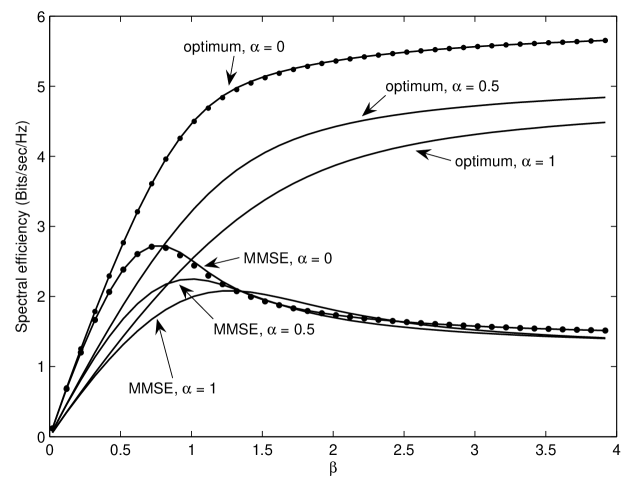
Figure 1: Large system spectral efficiencies of a chip-asynchronous CDMA system for $E_{b}/N_{0}=10$ dB and unfaded channel.

Fig. 1 shows the spectral efficiencies versus $\beta$ in a chip-asynchronous system for the optimum and the linear MMSE receivers, where $E_{b}/N_{0}$ is fixed as $10$ dB and an unfaded channel is assumed. Spectral efficiencies corresponding to SRRC pulses with different roll-off factors are depicted, and curves in the figure are obtained from (57) and (58) using a 10-point quadrature rule. The black dots on the figure are obtained from the analytical results

$${\cal C}^{\textsf{opt}}(\alpha=0,\beta,\textsf{\footnotesize SNR}) = \beta\log_{2}\left(1+\textsf{\footnotesize SNR}-\frac{1}{4}{\cal F}(\textsf{\footnotesize SNR},\beta)\right)+\log_{2}\left(1+\textsf{\footnotesize SNR}\beta-\frac{1}{4}{\cal F}(\textsf{\footnotesize SNR},\beta)\right)$$

$$-\frac{\log_{2}e}{4\textsf{\footnotesize SNR}}{\cal F}(\textsf{\footnotesize SNR},\beta)$$

and

$${\cal C}^{\textsf{mmse}}(\alpha=0,\beta,\textsf{\footnotesize SNR})=\beta\log_{2}\left(1+\textsf{\footnotesize SNR}-\frac{1}{4}{\cal F}(\textsf{\footnotesize SNR},\beta)\right)$$

when $\alpha=0$, where

$${\cal F}(x,z)=\left(\sqrt{x(1+\sqrt{z})^{2}+1}-\sqrt{x(1-\sqrt{z})^{2}+1}\right)^{2}.$$

These results are derived in [2] for a symbol-synchronous system. However, by Corollary 1, they are applicable to a chip-asynchronous system with $\alpha=0$ as well. It is seen that, when $\beta$ is around 1, there is visible discrepancy between results of the analytical formula and the Gauss quadrature method on the spectral efficiency of the MMSE receiver. This is because the Marc̆enko-Pastur distribution, i.e., the ASD corresponding to $\alpha=0$, tends to be infinite-interval when $\beta$ is close to 1, and the Gauss quadrature method is less accurate when the density function has an infinite interval.

The discussions in the following two paragraphs apply to chip-asynchronous systems. For the optimum receiver, given any $\beta$, the spectral efficiency corresponding to $\alpha=0$ is obviously greater than that of $\alpha=0.5$ and then of $\alpha=1$. The spectral efficiency grows as $\beta$ increases. When $\beta$ is small, the ratios of spectral efficiencies of $\alpha=0$, $0.5$ and $1$ are roughly equal to the ratios of inverses of their bandwidths, i.e., ratios of $(1+\alpha)^{-1}$, meaning the maximum bit rates that can be transmitted arbitrarily reliably are the same for various SRRC-$\alpha$ pulses, although the consumed bandwidths are different. As $\beta$ gradually increases, the ratios of spectral efficiencies ($\alpha=0$ to $0.5$ and to $1$) become smaller and smaller, suggesting that, when a chip waveform with a larger excess bandwidth is chosen, the the maximum reliable transmission rate can be increased.

For the linear MMSE receiver, the spectral efficiency is maximized by a certain $\beta$ depending on $\alpha$. When $\beta$ is small, it is obvious that chip waveforms with smaller values of $\alpha$ have larger MMSE spectral efficiencies. Nonetheless, as $\beta$ is greater than around $1.2$, the favor of smaller $\alpha$ in spectral efficiencies disappears. For low $\beta$, the linear MMSE receiver achieves near-optimum spectral efficiency. Otherwise, great gains in efficiency can be realized by nonlinear receivers. When $\beta$ is small, the MMSE receiver with $\alpha=0$ is superior to the optimum receiver having $\alpha=0.5$ in terms of spectral efficiency; so is the MMSE receiver with $\alpha=0.5$ to the optimum receiver having $\alpha=1$. Comparing curves of two receivers, we comment when more bandwidths are consumed due to the choice of an SRRC pulse with higher $\alpha$, the return in channel capacity (maximum reliable data rate) is larger in the linear MMSE receiver than in the optimum receiver. For example, when $\beta=2$, twice bandwidth of an SRRC pulse with $\alpha=1$ than with $\alpha=0$ results in approximately twice reliable data rate of $\alpha=1$ than $\alpha=0$ in the linear MMSE receiver. However, for the optimum receiver, the ratio of the data rates between $\alpha=1$ and $\alpha=0$ is around $1.5$ for the same $\beta$. Even for values of $\beta$ in a practical system, the higher return of the MMSE receiver in capacity is still true. Another interesting observation is that the MMSE spectral efficiency curve of SRRC pulse with $\alpha=1$ is above the curve of the sinc pulse in the region around $\beta\in[1.5,2]$. However, as the difference of the two curves is small, we should be careful in making comments. In that region, the curve of the sinc pulse is exact (matching with the analytical result); the curve of SRRC with $\alpha=1$ is an approximation with two opposite forces counter-acting on each other. On the one hand, (58) is a lower bound so the curve underestimates the true spectral efficiency; on the other hand, the numerical method tends to be optimistic, which yields an overestimate. We surmise that the first factor dominates; adding the result that the curve of sinc pulse is below the other, we conjecture: for some $\beta$, the sinc pulse is not optimal in terms of the MMSE spectral efficiency under the indicated environments.

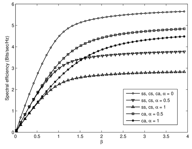
Figure 2: Large system optimum spectral efficiencies of symbol-synchronous, chip-synchronous, and chip-asynchronous CDMA systems when $E_{b}/N_{0}=10$ dB and the channel is unfaded, where ”ss”, ”cs” and ”ca” refer to symbol-synchronous, chip-synchronous, and chip-asynchronous, respectively.

Fig. 2 shows the optimum spectral efficiencies as a function of $\beta$ for symbol-synchronous, chip-synchronous and chip-asynchronous systems with various chip waveforms when $E_{b}/N_{0}=10$ dB and the channel is unfaded. The three curves marked by circles, squares and stars have appeared in Fig. 1; those two marked by triangles (down and up) are obtained from (57), where $\lambda_{{\boldsymbol{R}}_{\textrm{ca},\alpha}}$ in the equation is replaced with $\lambda_{{\boldsymbol{R}}_{\textrm{cs},\alpha}}$. In both symbol- and chip-synchronous systems, the spectral efficiency corresponding to a particular $\alpha^{*}$ is equal to the spectral efficiency corresponding to $\alpha=0$ divided by $1+\alpha^{*}$. This is because $\lambda_{{\boldsymbol{R}}_{\textrm{cs},\alpha}}$ has the same distribution regardless of $\alpha$.

When $\alpha=0$, three systems have the same optimum spectral efficiency. This is a direct consequence of Corollary 2. Given any $\alpha$, when $\beta$ is low, the differences of the three systems in optimum spectral efficiency are negligible; as $\beta$ increases, the chip-asynchronous system is superior to the other two for nonzero $\alpha$, and the optimum spectral efficiency differences are proportional to $\beta$. On the other hand, given any $\beta$, as $\alpha$ increases, the chip-asynchronous system has a larger spectral efficiency than the other two, and the difference grows with $\alpha$. Similar comments can be made from Fig. 1 for the MMSE spectral efficiencies of the three systems. We also observe, while choosing chip waveforms with larger bandwidths may result in the increase of channel capacity in a chip-asynchronous system, the statement is not true for symbol- and chip-synchronous systems. This can be interpreted as follows. It is the ASD that determines the performance measures of a system such as the channel capacity, the MMSE achievable by a linear receiver, and so on. Regretfully, the ASD of symbol- and chip-synchronous systems does not depend on the chosen chip waveform; hence the increase of bandwidth due to the replacement of a chip waveform merely decreases the spectral efficiency and does not help in boosting the capacity.

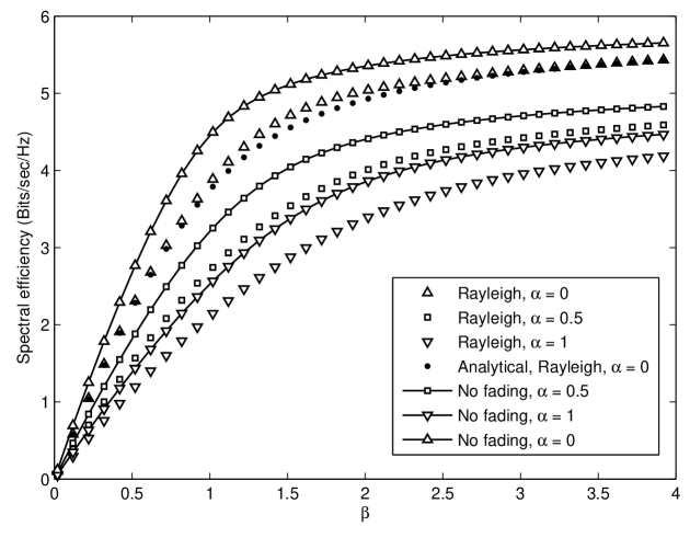
Figure 3: Large system optimum spectral efficiencies of a chip-asynchronous system for unfaded and Rayleigh fading channels when $E_{b}/N_{0}=10$ dB.

Consider a channel subject to frequency-flat fading. The square magnitude of the received signal $|A_{k}(m)|^{2}$ is governed by SNR common to all users and a normalized random variable $\overline{A}_{k}(m)$ having $\textrm{E}\{|\overline{A}_{k}(m)|^{2}\}=1$. Thus, the amplitude matrix ${\boldsymbol{A}}$ has ${\boldsymbol{A}}{\boldsymbol{A}}^{\dagger}=\textsf{\footnotesize SNR}\overline{{\boldsymbol{A}}}\overline{{\boldsymbol{A}}}^{\dagger}$, where $\overline{{\boldsymbol{A}}}$ has the same structure as the diagonal amplitude matrix ${\boldsymbol{A}}$, and $\overline{A}_{k}(m)$ is located at the $(k,k)$-th entry in the $(m,m)$-th block of $\overline{{\boldsymbol{A}}}$. The spectral efficiencies of the optimum receiver is given by (57) with $\lambda_{{\boldsymbol{R}}_{\textrm{ca},\alpha}}$ replaced as $\lambda_{\overline{{\boldsymbol{A}}}^{\dagger}{\boldsymbol{R}}_{\textrm{ca},\alpha}\overline{{\boldsymbol{A}}}}$. Although we can also modify (58) to yield a lower bound for the MMSE spectral efficiency under fading; however, according to our experiments, the bound is loose. Fig. 3 compares optimum spectral efficiencies in a chip-asynchronous system with and without fading for a fixed $E_{b}/N_{0}$ equal to $10$ dB. The fading channel is assumed to be Rayleigh. To generate curves of the fading channel, a 15-point quadrature rule is used. The black dots shown in the figure correspond to the analytical result obtained in [45] for $\alpha=0$ and a Rayleigh fading channel. Perceptible discrepancy between analytical and numerical results appear in the region of $\beta\in[1,2]$. We comment that fading in a chip-asynchronous system leads to a degradation in optimum spectral efficiency, which is consistent with a mathematical result demonstrated in [45].

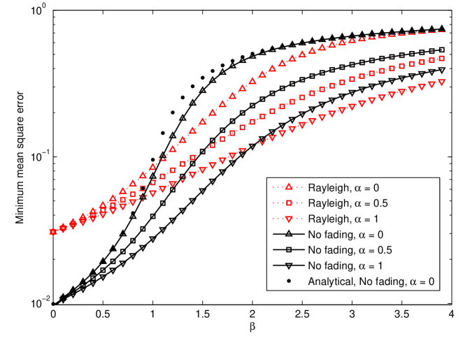
Figure 4: Large system MMSE versus $\beta$ of a chip-asynchronous system for unfaded and Rayleigh fading channels when $\textsf{\footnotesize SNR}=20$ dB.

In the presence of fading, the arithmetic mean over the users of the mean-square-error achieved by the linear MMSE receiver is given as [5]

$${\cal E}(\alpha,\beta,\textsf{\footnotesize SNR})=\textrm{E}\left\{\frac{1}{1+\textsf{\footnotesize SNR}\cdot\lambda_{\overline{{\boldsymbol{A}}}^{\dagger}{\boldsymbol{R}}_{\textrm{ca},\alpha}\overline{{\boldsymbol{A}}}}}\right\}.$$ (59)

For the unfaded case, ${\cal E}(\alpha,\beta,\textsf{\footnotesize SNR})$ is obtained by setting $\overline{{\boldsymbol{A}}}$ in (59) as the identity matrix. Fig. 4 compares the MMSE achievable by a linear receiver for unfaded and Rayleigh fading channels when $\textsf{\footnotesize SNR}=20$ dB. We use 10- and 15-point quadrature rules for unfaded and fading channels, respectively. Black dots on the figure correspond to the analytical result of

$$1-\frac{{\cal F}(\textsf{\footnotesize SNR},\beta)}{4\beta\textsf{\footnotesize SNR}}$$

for $\alpha=0$ in the absence of fading [2]. According to our tests, the discrepancy between the analytical and numerical results grows with SNR. The difference becomes almost unnoticeable when $\textsf{\footnotesize SNR}<15$ dB. For low $\beta$, the MMSE in an unfaded channel is lower than in a Rayleigh fading channel. In the latter case, as $\beta\to 0$, the analytical result is equal to $\textrm{E}\{(1+\textsf{\footnotesize SNR}\cdot X)^{-1}\}=0.04079$, where $X$ has the exponential density $e^{-x}$, $x\geq 0$; the numerical result is equal to $0.03075$ at $\beta\to 0$.

We observe that, regardless of fading or not, the MMSE is inversely proportional to $\alpha$ in a chip-asynchronous system. This is consistent with the conclusion drawn previously that choosing chip waveforms with larger excess bandwidths leads to a higher capacity. Nevertheless, for symbol- and chip-synchronous systems, regardless of $\alpha$, the MMSE are unchanged and correspond to the curve of $\alpha=0$. Interestingly, we can see that fading decreases the MMSE in the region of high $\beta$. The explanation is similar to that for fading increasing the spectral efficiency at high $\beta$ made in [45]. That is, due to fading, a certain portion of interferers are low-powered; thus, the number of ”effective” interferers seen by the receiver is reduced. This interference population control of fading compensates for its harmful effect on the desired user. It is also observed, as $\alpha$ increases, the receiver needs a larger $\beta$ to have this phenomenon begin to operate, and this phenomenon is less obvious for larger $\alpha$.

VII Conclusion

In this paper, the ASD of crosscorrelation matrices in random spreading chip-synchronous and chip-asynchronous CDMA systems are investigated with a particular emphasis on the derivation of AEM. Noncrossing partition and the graphical representation of $K$-graph are the key tools in AEM computation. We assume an infinite observation window width, known spreading sequences and relative delays to the receiver, and an arbitrary chip waveform. We consider both unfaded and frequency-flat fading channels. The spreading sequences are only assumed to be independent across users. For a particular user, we do not assume that the sequence is independent across symbols. Thus, results shown in this paper are applicable for both short-code and long-code systems.

In the following, results of this paper are summarized. For chip-synchronous CDMA systems, the explicit expressions for AEM of the crosscorrelation matrix are given when the users’ relative delays are deterministic constants. We show that AEM do not depend on the realizations of asynchronous delays and the shape of chip waveform, as long as the zero ICI condition holds. It is also shown that the AEM formulas are identical to those of symbol-synchronous CDMA. In an unfaded channel, as the AEM satisfy the Carleman’s criterion and the a.s. convergence test, it is concluded that the ASD in a chip-synchronous system converges a.s. to Marc̆enko-Pastur law with ratio index $\beta$. In the case of flat fading, the a.s. convergence of ESD to a nonrandom ASD is established provided that a constraint on the empirical moments of the fading coefficients is satisfied.

For chip-asynchronous CDMA systems, the convergence of ESD to an ASD in a.s. sense is proved for general constraints on the chip waveform and, for a fading channel, the empirical moments of the signal received power. It is shown that, in contrast to chip-synchronous CDMA, AEM in a chip-asynchronous system are dependent on the shape of chip waveform. On the other hand, the relation of AEM and users’ relative delays depends on the bandwidth of the chosen chip waveform. Specifically, it is mentioned that, for the zero ICI property to hold, the chip waveform has a bandwidth at least equal to $1/(2T_{c})$, which corresponds to the sinc pulse. When the bandwidth of the chip waveform is $1/(2T_{c})$, AEM do not depend on the realizations of relative delays. On the contrary, if the bandwidth is wider than the threshold, AEM do depend on the asynchronous delays; nonetheless, different relative delays realizations may result in the same AEM. Suppose that relative delays are modeled as i.i.d. random variables $\tau_{k}$’s. Let $G_{1}$ and $G_{2}$ be two distinct distributions of relative delays, and both of them possess the symmetry property of $\textrm{E}\left\{\cos(2\pi n\tau_{k}/T_{c})\right\}=0$ for nonzero integer $n$. Then, for the same chip waveform, AEM’s averaged over realizations of relative delays with distributions $G_{1}$ and $G_{2}$ are equal. The distribution symmetry condition given above encompasses the symbol quasi-synchronous but chip-asynchronous system considered in [18]. By moment convergence theorem, the equivalence of AEM leads to an equivalence of ASD provided that the uniqueness of limiting distribution is true. It follows that our result proves the conjecture given there that relative delays ranging uniformly within the chip duration and within the symbol duration yield the same performance. When the sinc chip waveform is adopted, no matter fading or not, the AEM of chip-asynchronous CDMA are shown to be equal to those of chip-synchronous CDMA and hence those of a symbol-synchronous system. This explains the equivalence result of [16] that the output SIR of the linear MMSE receiver converges to those of chip- and symbol-synchronous systems when $M$ is large. Since every receiver in the family constructed in [39] can be arbitrarily well approximated by a polynomial receiver, and both the polynomial coefficients and the polynomial receiver’s output SIR are determined by AEM, we can also prove the conjecture in [16] that the equivalence result in the output SIR of the three systems holds for all receivers in that family. We also study the situation that the chip waveform bandwidth is less than $1/(2T_{c})$ such that zero ICI condition is lost. It is shown that, without the zero ICI property, the AEM formulas in symbol- and chip-synchronous systems bear the same forms as those in a chip-asynchronous system. Thus, when systems of three synchronism levels have the same parameters except for the delays of the users, their AEM’s are all the same; consequently, these three systems have the same ASD.

With the help of free probability theory, free cumulants of crosscorrelation matrices are also derived for both chip-synchronous and chip-asynchronous systems. It is also proved that the crosscorrelation matrix is asymptotically free with a random diagonal matrix having a general constraint. Based on the asymptotic freeness property, AEM’s for the sum and the product of the crosscorrelation matrix and a random diagonal matrix are derived accordingly.

Mathematical results obtained in this paper are connected to those that are widely used by researchers who apply random matrix theory to communication problems.

At last, some application cases are provided. The Gauss quadrature rule method is adopted to depict the spectral efficiencies of the optimum and linear MMSE detectors and the MMSE achievable by a linear receiver in asynchronous CDMA. Performance in the measures of the spectral efficiency, channel capacity, and MMSE are compared for various chip waveforms, two types of receivers, and different asynchronism levels.

Appendix A Noncrossing Partition

The proofs of Lemmas 1 and 5 require results from noncrossing partition of set partition theory. Our treatment here for noncrossing partition is very brief; for more details, please consult [46].

Definition 2

(Noncrossing Partition [29,46]) Let $S$ be a finite totally ordered set.

1. We call $\varpi=\{B_{1},\cdots,B_{j}\}$ a partition of the set $S$ if and only if $B_{1},\cdots,B_{j}$ are pairwise disjoint, non-empty subsets of $S$ such that $B_{1}\cup\cdots\cup B_{j}=S$. We call $B_{1},\cdots,B_{j}$ the classes of $\varpi$. The classes $B_{1},\cdots,B_{j}$ are ordered according to the minimum element in each block. That is, the minimum element in $B_{k}$ is smaller than that of $B_{l}$ if $k<l$.

2. The collection of all partitions of $S$ can be viewed as a partially ordered set (poset) in which the partitions are ordered by refinement: if $\varpi,\sigma$ are two partitions of $S$, we have $\varpi\leq\sigma$ if each block of $\varpi$ is contained in a block of $\sigma$. For example, when $S=\{1,2,3,4,5,6,7\}$, we have $\{\{1\},\{2,5\},\{3,4\},\{6\},\{7\}\}<\{\{1,3,4\},\{2,5\},\{6,7\}\}$.

3. A partition of the set $S$ is called crossing if there exist $p_{1}<q_{1}<p_{2}<q_{2}$ in $S$ such that $p_{1}$ and $p_{2}$ belong to one class and $q_{1}$ and $q_{2}$ to another. If a partition is not crossing, then it is called noncrossing. $\blacksquare$

The set of all noncrossing partitions of $S$ is denoted by $\mathit{NC}(S)$. In the special case $S=\{1,\cdots,n\}$, we denote this by $\mathit{NC}(n)$.

Definition 3

(Kreweras Complementation Map [29,46]) Consider elements $\overline{1},\overline{2},\cdots,\overline{n}$ and interlace them with $1,2,\cdots,n$ in the alternating way of $1,\overline{1},2,\overline{2},\cdots,n,\overline{n}$. Let $\varpi\in\mathit{NC}(n)$. Then its Kreweras complementation map $\mathit{KC}(\varpi):\mathit{NC}(n)\rightarrow\mathit{NC}(n)\in\mathit{NC}(\{\overline{1},\overline{2},\cdots,\overline{n}\})$ is defined as the biggest element among those $\sigma\in\mathit{NC}(\{\overline{1},\overline{2},\cdots,\overline{n}\})$ such that the union $\varpi\cup\sigma$ of the two noncrossing partitions belongs to $\mathit{NC}(\{1,\overline{1},2,\overline{2},\cdots,n,\overline{n}\})$. $\hfill{\small\blacksquare}$

It can be shown that, if $\varpi$ contains $j$ classes, then the number of classes in $\mathit{KC}(\varpi)$ is $n-j+1$.

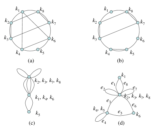
Figure 5: (a) The partition $\{\{k_{1},k_{4},k_{6}\}\{k_{2},k_{3},k_{7},k_{8}\}\{k_{5}\}\}$ of the totally ordered set $\{k_{1},k_{2},\cdots,k_{8}\}$, (b) the partition $\{\{k_{1}\}\{k_{2},k_{3},k_{7},k_{8}\}\{k_{4},k_{5}\}\{k_{6}\}\}$, (c) the $K$-graph for the partition represented in (a), and (d) the $K$-graph for the partition represented in (b).

A partition can be represented graphically. For example, Figs. 5(a) and 5(b) show two partitions of $\{k_{1},k_{2},\cdots,k_{8}\}$, where elements in the same class are joined successively by chords. A noncrossing partition is such that the chords intersect only at elements $k_{1},\cdots,k_{n}$. For instance, Fig. 5(b) is a noncrossing partition, while Fig. 5(a) is not. In the following, we define a representation, called $K$-graph, for any partition of a totally ordered set. The $K$-graph defined below is similar to the $W$-graph of [33] used to establish the convergence of moments of a Wigner matrix. We discover several pleasant properties of $K$-graphs that will be useful in proving the lemmas. They are enumerated right after the definition of $K$-graph.

Definition 4

($K$-graph) The $K$-graph corresponding to a partition $\varpi=\{B_{1},\cdots,B_{j}\}$ of a totally ordered set $\{k_{1},k_{2},\cdots,k_{n}\}$ is denoted by a graph $G=({\cal V},{\cal E})$. The vertex set is ${\cal V}=\{v_{1},v_{2},\cdots,v_{j}\}$, and the edge set is ${\cal E}=\{e_{1},e_{2},\cdots,e_{n}\}$, where the edge $e_{r}$ connects vertices $v_{s}$ and $v_{t}$ if $k_{r}$ and $k_{r+1}$ are partitioned into classes $B_{s}$ and $B_{t}$, respectively (with $n+1:=1$). $\hfill{\small\blacksquare}$

Remark: The $K$-graph for a partition $\varpi$ of $\{k_{1},k_{2},\cdots,k_{n}\}$ can be interpreted in a more visually convenient way as follows. Let $k_{i}$’s be arranged orderly (either clockwise or counter-clockwise) as vertices of an $n$-vertex cycle, and let edge $e_{r}$ connect vertices $k_{r}$ and $k_{r+1}$. The $K$-graph of $\varpi$ can be obtained by merging vertices that are partitioned in the same class of $\varpi$ into one. When vertices are merged, edges originally incident on these vertices become incident on the merged one. Mergence of two adjacent vertices results in a self-loop cycle. $\blacksquare$

For example, Figs. 5(c) and 5(d) present the $K$-graphs for the partitions of Figs. 5(a) and 5(b), respectively.

Properties of $K$-graphs: Given a partition $\varpi$ of a totally ordered $n$-element set ${\cal K}$ and its corresponding $K$-graph $G=({\cal V},{\cal E})$. We have the following properties.

1. There is a bijective correspondence between classes of $\varpi$ and vertices of $G$.

2. $G$ is connected. If and only if $\varpi$ is noncrossing, $G$ is a concatenation of cycles with any two of them connected by at most one vertex. Moreover, if $\varpi$ is noncrossing and has $j$ classes, then there are $n-j+1$ cycles in $G$. For example, Fig. 5(d) is composed of $8-4+1=5$ cycles. Any pair of these five cycles are connected by at most one of the two vertices labelled with $k_{2},k_{3},k_{7},k_{8}$ and $k_{4},k_{5}$.

3. Consider a partition $\sigma$ of the ordered edge set ${\cal E}=\{e_{1},e_{2},\cdots,e_{n}\}$ of $G$ by letting edges in the same cycle of $G$ being in the same class. If $\varpi$ is noncrossing, then $\sigma$ is noncrossing as well. Moreover, $\varpi$ and $\sigma$ are Kreweras complementation maps of each other. For example, Fig. 5(d) corresponds to $\sigma=\{\{e_{1},e_{8}\},\{e_{2}\},\{e_{3},e_{5},e_{6}\},$ $\{e_{4}\},\{e_{7}\}\}$, which is a noncrossing partition of $\{e_{1},e_{2},\cdots,e_{8}\}$. It is seen that $\{\{1,8\},\{2\},\{3,5,6\},\{4\},\{7\}\}$ is the Kreweras complementation map of $\{\{1\},\{2,3,7,8\},$ $\{4,5\},\{6\}\}$, and vice versa. $\blacksquare$

From properties 1) and 3), if $\varpi$ is noncrossing, then the corresponding $K$-graph can represent both $\varpi$ and its Kreweras complementation map simultaneously. That is, $\varpi$ and $\mathit{KC}(\varpi)$ can be identified by the vertex set and edge set of the $K$-graph, respectively.

Some results about noncrossing partition are in order. The number of noncrossing partitions that partition $n$ elements into $j$ classes is the Narayana number, given by

$$\dfrac{1}{n}{n\choose j}{n\choose j-1}.$$ (60)

Moreover, if the $j$ classes have sizes $c_{1},c_{2},\cdots,c_{j}$ with $c_{1}\geq c_{2}\geq\cdots\geq c_{j}\geq 1$ (but not specifying which class gets which size), the number of noncrossing partitions is [29]

$$\dfrac{n(n-1)\cdots(n-j+2)}{f(c_{1},c_{2},\cdots,c_{j})},$$ (61)

where

$$f(c_{1},c_{2},\cdots,c_{j})=\prod_{k\geq 1}n_{k}!$$ (62)

with $n_{k}$ being the number of elements in $(c_{1},c_{2},\cdots,c_{j})$ that are equal to $k$. It is clear to see

$$\mathop{\sum_{c_{1}+c_{2}+\cdots+c_{j}=n}}_{c_{1}\geq c_{2}\geq\cdots\geq c_{j}\geq 1}\dfrac{n(n-1)\cdots(n-j+2)}{f(c_{1},c_{2},\cdots,c_{j})}=\dfrac{1}{n}{n\choose j}{n\choose j-1}.$$ (63)

The number of noncrossing partitions $\varpi$ of an $n$-element set meeting conditions of

1. $\varpi$ has $j$ classes with sizes in non-ascending order of $(c_{1},c_{2},\cdots,c_{j})$, and

2. the classes of $\mathit{KC}(\varpi)$ have sizes in non-ascending order of $(b_{1},b_{2},\cdots,b_{n-j+1})$,

is equal to [47,12]

$$\dfrac{n(n-j)!(j-1)!}{f(b_{1},b_{2},\cdots,b_{n-j+1})f(c_{1},c_{2},\cdots,c_{j})}.$$ (64)

Appendix B Proofs of Lemma 1 and Lemma 5

With the results of noncrossing partition in Appendix A, we now proceed to prove Lemma 1 and Lemma 5. Consider $\mu({\boldsymbol{R}}_{\textrm{cs}}^{n})$ in (24) and $\mu({\boldsymbol{R}}_{\textrm{ca}}^{n})$ by replacing ${\boldsymbol{R}}_{\textrm{cs}}$ in the equation with ${\boldsymbol{R}}_{\textrm{ca}}$. They can be rewritten as

$$\mu({\boldsymbol{R}}_{\textrm{x}}^{n})=\mathop{\lim_{K,N\rightarrow\infty}}_{K/N\rightarrow\beta}K^{-1}\left[\lim_{M\rightarrow\infty}(2M+1)^{-1}\textrm{E}\left\{\operatorname{tr}(({\boldsymbol{R}}_{\textrm{x}}^{(K)})^{n})\right\}\right],\quad\textrm{x}\in\{\textrm{cs},\textrm{ca}\}.$$ (65)

For notational convenience, the superscript ^(K) of ${\boldsymbol{R}}_{\textrm{x}}^{(K)}$ will be omitted below when no ambiguity occurs. By (7) and (13), we have

$$[{\boldsymbol{R}}_{\textrm{cs}}]_{m_{r}m_{r+1},k_{r}k_{r+1}}\hskip 5.69054pt=\hskip 5.69054pt\rho_{\textrm{cs}}(m_{r},m_{r+1};k_{r},k_{r+1})$$

$$= \sum_{p_{r}=m_{r}N}^{(m_{r}+1)N-1}\sum_{q_{r+1}=m_{r+1}N}^{(m_{r+1}+1)N-1}c_{k_{r}}^{(p_{r})}c_{k_{r+1}}^{(q_{r+1})}\delta(p_{r}T_{c}+\tau_{k_{r}},q_{r+1}T_{c}+\tau_{k_{r+1}}),$$

and

$$[{\boldsymbol{R}}_{\textrm{ca}}]_{m_{r}m_{r+1},k_{r}k_{r+1}}\hskip 5.69054pt=\hskip 5.69054pt\rho_{\textrm{ca}}(m_{r},m_{r+1};k_{r},k_{r+1})$$

$$= \sum_{p_{r}=m_{r}N}^{(m_{r}+1)N-1}\sum_{q_{r+1}=m_{r+1}N}^{(m_{r+1}+1)N-1}c_{k_{r}}^{(p_{r})}c_{k_{r+1}}^{(q_{r+1})}R_{\psi}((p_{r}-q_{r+1})T_{c}+\tau_{k_{r}}-\tau_{k_{r+1}}),$$

for $1\leq r\leq n$ with $m_{n+1}:=m_{1}$ and $k_{n+1}:=k_{1}$. By expanding matrix multiplications of ${\boldsymbol{R}}_{\textrm{x}}^{n}$, the term inside of square brackets of (65) can be expressed as

$$\lim_{M\rightarrow\infty}(2M+1)^{-1}\textrm{E}\left\{\operatorname{tr}(\boldsymbol{R}_{\textrm{x}}^{n})\right\}$$ (66)

$$= \lim_{M\rightarrow\infty}(2M+1)^{-1}\sum_{{\cal K}\in{\cal X}}\sum_{{\cal M}\in{\cal Y}}\textrm{E}\{[\boldsymbol{R}_{\textrm{x}}]_{m_{1}m_{2},k_{1}k_{2}}[\boldsymbol{R}_{\textrm{x}}]_{m_{2}m_{3},k_{2}k_{3}}\cdots[\boldsymbol{R}_{\textrm{x}}]_{m_{n}m_{1},k_{n}k_{1}}\},$$

where ${\cal K}=\{k_{1},\cdots,k_{n}\}$, ${\cal X}=\underbrace{[1,K]\times\cdots\times[1,K]}_{n\textrm{ times}}=[1,K]^{n}$, ${\cal M}=\{m_{1},\cdots,m_{n}\}$ and ${\cal Y}=[-M,M]^{n}$. Equation (66) is equal to

$$\lim_{M\rightarrow\infty}(2M+1)^{-1}\sum_{{\cal K}\in{\cal X}}\sum_{{\cal M}\in{\cal Y}}\sum_{{\cal P}_{1}\in{\cal Z}_{1}}\cdots\sum_{{\cal P}_{n}\in{\cal Z}_{n}}\textrm{E}\left\{\left(c_{k_{1}}^{(p_{1})}c_{k_{2}}^{(q_{2})}\right)\left(c_{k_{2}}^{(p_{2})}c_{k_{3}}^{(q_{3})}\right)\cdots\left(c_{k_{n}}^{(p_{n})}c_{k_{1}}^{(q_{1})}\right)\right\}$$

$$\times\delta(p_{1}T_{c}+\tau_{k_{1}},q_{2}T_{c}+\tau_{k_{2}})\delta(p_{2}T_{c}+\tau_{k_{2}},q_{3}T_{c}+\tau_{k_{3}})\cdots\delta(p_{n}T_{c}+\tau_{k_{n}},q_{1}T_{c}+\tau_{k_{1}}),$$ (67)

when $\textrm{x}=\textrm{cs}$, and

$$\lim_{M\rightarrow\infty}(2M+1)^{-1}\sum_{{\cal K}\in{\cal X}}\sum_{{\cal M}\in{\cal Y}}\sum_{{\cal P}_{1}\in{\cal Z}_{1}}\cdots\sum_{{\cal P}_{n}\in{\cal Z}_{n}}\textrm{E}\left\{\left(c_{k_{1}}^{(p_{1})}c_{k_{2}}^{(q_{2})}\right)\left(c_{k_{2}}^{(p_{2})}c_{k_{3}}^{(q_{3})}\right)\cdots\left(c_{k_{n}}^{(p_{n})}c_{k_{1}}^{(q_{1})}\right)\right\}$$ (68)

$$\times\textrm{E}\{R_{\psi}((p_{1}-q_{2})T_{c}+\tau_{k_{1}}-\tau_{k_{2}})R_{\psi}((p_{2}-q_{3})T_{c}+\tau_{k_{2}}-\tau_{k_{3}})\cdots R_{\psi}((p_{n}-q_{1})T_{c}+\tau_{k_{n}}-\tau_{k_{1}})\},$$

when $\textrm{x}=\textrm{ca}$, where ${\cal P}_{r}=\{p_{r},q_{r}\}$ and ${\cal Z}_{r}=[m_{r}N,(m_{r}+1)N-1]^{2}$ for $1\leq r\leq n$. Owing to the tri-diagonal structure of $\boldsymbol{R}_{\textrm{cs}}$ shown in (10), there are constraints $|m_{r}-m_{r+1}|\leq 1$ for $1\leq r\leq n$ when (67) is considered. Moreover, as stated in the beginning of Section III-B, the relative delays $\tau_{k}$’s are viewed as deterministic when the chip waveform is the ideal sinc pulse and viewed as random when otherwise, the expectation in the second line of (68) can be discarded when the sinc pulse is adopted.

Computations of (67) and (68) can be executed by considering the equivalence patterns of elements in ${\cal K}=\{k_{1},k_{2},\cdots,k_{n}\}$. As equivalence relation and partition are essentially equivalent, the computations of (67) and (68) can be carried out with the aid of set partition theory, where $\cal K$ is a totally ordered set with ordering $k_{1}\succ k_{2}\succ\cdots\succ k_{n}$, and $k_{r}$ and $k_{s}$ are partitioned in the same class if and only if they take the same integer in $[1,K]$. Note that the ordering $k_{1}\succ k_{2}\succ\cdots\succ k_{n}$ is just an arrangement of objects $k_{i}$’s as an ordered set. It is different from the ordering of the values taken by summation variables $k_{1},k_{2},\cdots,k_{n}$ in $[1,K]$.

In the following, the summation $\sum_{{\cal K}\in{\cal X}}$ in (67) and (68) is decomposed into several ones using properties stated in Appendix A. Let ${\cal X}_{j}\subseteq{\cal X}=[1,K]^{n}$ such that each element $x_{j}=(x_{j}(1),\cdots,x_{j}(n))$ in ${\cal X}_{j}$ corresponds to a $j$-class noncrossing partition of an $n$-element ordered set. We mean $x_{j}$ corresponds to a partition by that $x_{j}(s)=x_{j}(t)$ if and only if the $s$- and $t$-th elements are partitioned in the same class in that partition. Moreover, let ${\cal X}_{j}(b_{1},b_{2},\cdots,b_{n-j+1})$, with $b_{1}\geq b_{2}\geq\cdots\geq b_{n-j+1}\geq 1$, stand for the union of $x_{j}$’s whose corresponding noncrossing partitions have Kreweras complementation maps with class sizes $(b_{1},b_{2},\cdots,b_{n-j+1})$ (but not specifying which class gets which size). Since the Kreweras complementation map of a noncrossing partition is noncrossing as well, by (61), the number of elements in ${\cal X}_{j}(b_{1},b_{2},\cdots,b_{n-j+1})$ is given by

$$\#{\cal X}_{j}(b_{1},b_{2},\cdots,b_{n-j+1})=\dfrac{n(n-1)\cdots(j+1)}{f(b_{1},b_{2},\cdots,b_{n-j+1})}\cdot K(K-1)\cdots(K-j+1).$$

The above equation is interpreted as follows. The number of noncrossing partitions associated with ${\cal X}_{j}(b_{1},b_{2},\cdots,b_{n-j+1})$ is $n(n-1)\cdots(j+1)/f(b_{1},b_{2},\cdots,b_{n-j+1})$, and each of these noncrossing partitions has $j$ classes, with each class specified by a distinct integer in $[1,K]$. Moreover, let ${\cal X}_{cro}\subseteq{\cal X}$, where each element in ${\cal X}_{cro}$ corresponds to a crossing partition of an $n$-element ordered set. With these settings, the summation $\sum_{{\cal K}\in{\cal X}}$ in (67) and (68) can be decomposed as

$$\sum_{{\cal K}\in{\cal X}}\hskip 8.53581pt\equiv\hskip 8.53581pt\sum_{j=1}^{n}\hskip 5.69054pt\mathop{\sum_{b_{1}+b_{2}+\cdots+b_{n-j+1}=n}}_{b_{1}\geq b_{2}\geq\cdots\geq b_{n-j+1}\geq 1}\hskip 5.69054pt\sum_{{\cal K}\in{\cal X}_{j}(b_{1},b_{2},\cdots,b_{n-j+1})}+\sum_{{\cal K}\in{\cal X}_{cro}}.$$ (69)

Now, we consider $K$-graphs corresponding to elements of ${\cal X}_{j}(b_{1},b_{2},\cdots,b_{n-j+1})$ and of ${\cal X}_{cro}$ in (69). To embed the summation variables $p_{r}$’s and $q_{r}$’s of (67) and (68) into a $K$-graph, in the $n$-vertex cycle composed of vertices $k_{1},k_{2},\cdots,k_{n}$, two ends of the edge connecting $k_{r}$ and $k_{r+1}$ are labelled with $p_{r}$ and $q_{r+1}$, with the former and latter touching $k_{r}$ and $k_{r+1}$, respectively. We call these $p_{r}$’s and $q_{r}$’s as edge variables. Fig. 6(a) shows the graph with edge variables labelled. The edge connecting vertices $k_{r}$ and $k_{r+1}$ stands for

$$c_{k_{r}}^{(p_{r})}c_{k_{r+1}}^{(q_{r+1})}\cdot\delta(p_{r}T_{c}+\tau_{k_{r}},q_{r+1}T_{c}+\tau_{k_{r+1}})$$

and

$$c_{k_{r}}^{(p_{r})}c_{k_{r+1}}^{(q_{r+1})}\cdot R_{\psi}((p_{r}-q_{r+1})T_{c}+\tau_{k_{r}}-\tau_{k_{r+1}})$$

in (67) and (68), respectively, and the summands in the equations are yielded by multiplying terms associated with all of the edges together. Vertices $k_{r}$’s and edge variables $p_{r}$’s, $q_{r}$’s in Fig. 6(a) are all summation variables of (67) and (68). Another set of summation variables $m_{r}$’s are implicitly embedded in $p_{r}$’s and $q_{r}$’s by that the ranges of $p_{r}$ and $q_{r}$ are both $[m_{r}N,(m_{r}+1)N-1]$. We would like to inspect under what equivalence relation of $p_{r}$’s and $q_{r}$’s would the contributions to (67) and (68) become nonvanishing in the large-system limit.

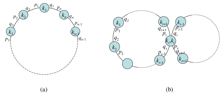
Figure 6: The $K$-graphs of (a) $n$-class partition $\{\{k_{1}\},\{k_{2}\},\cdots,\{k_{n}\}\}$, and (b) $(n-1)$-class partition $\{\{k_{1}\},\{k_{2}\},\cdots,\{k_{s},k_{t}\},\cdots,\{k_{n}\}\}$ with $s<t$.

B-A Contributions of Noncrossing Partitions to $\mu({\boldsymbol{R}}_{\textrm{cs}}^{n})$ and $\mu({\boldsymbol{R}}_{\textrm{ca}}^{n})$

To compute the contribution of noncrossing partitions of ${\cal K}=\{k_{1},k_{2},\cdots,k_{n}\}$ to $\mu({\boldsymbol{R}}_{\textrm{cs}}^{n})$ and $\mu({\boldsymbol{R}}_{\textrm{ca}}^{n})$, we replace $\sum_{{\cal K}\in{\cal X}}$ in (67) and (68) with the first term at the right-hand-side of (69) and then use (65). Given non-ascending ordered natural numbers $(b_{1},b_{2},\cdots,b_{n-j+1})$ such that $b_{1}+b_{2}+\cdots+b_{n-j+1}=n$. The contribution of each element of ${\cal X}_{j}(b_{1},b_{2},\cdots,b_{n-j+1})$ to (67) and (68) is to be evaluated. First, we consider $j=n$. There is only one $K$-graph, shown in Fig. 6(a). Since all of $k_{1},k_{2},\cdots,k_{n}$ are distinct, the expectations of spreading sequences in (67) and (68) are nonzero (equal to $N^{-n}$) if and only if $p_{r}=q_{r}$ for $1\leq r\leq n$. Note that, since $c_{k_{r}}^{(p_{r})}$ and $c_{k_{r}}^{(q_{r})}$ are chips in the same transmitted symbol, i.e., $m_{r}N\leq p_{r},q_{r}\leq(m_{r}+1)N-1$, the necessary and sufficient condition $p_{r}=q_{r}$ stated above holds for both short-code and long-code systems. The contribution of each element of ${\cal X}_{n}(n)$ to (67) becomes

$$N^{-n}\lim_{M\rightarrow\infty}(2M+1)^{-1}\sum_{{\cal M}\in{\cal Y}}\sum_{p_{1}\in{\cal Z}^{\prime}_{1}}\sum_{p_{2}\in{\cal Z}^{\prime}_{2}}\cdots\sum_{p_{n}\in{\cal Z}^{\prime}_{n}}\delta(p_{1}T_{c}+\tau_{k_{1}},p_{2}T_{c}+\tau_{k_{2}})$$

$$\times\delta(p_{2}T_{c}+\tau_{k_{2}},p_{3}T_{c}+\tau_{k_{3}})\cdots\delta(p_{n}T_{c}+\tau_{k_{n}},p_{1}T_{c}+\tau_{k_{1}}),$$ (70)

where ${\cal Z}^{\prime}_{r}=[m_{r},(m_{r}+1)N-1]$ and $|m_{r}-m_{r+1}|\leq 1$. The product of $\delta(\cdot,\cdot)$’s is nonzero and equal to one if and only if all $p_{r}T_{c}+\tau_{k_{r}}$, $1\leq r\leq n$, are equal. Since we have $p_{1}\in[m_{1}N,(m_{1}+1)N-1]$ for each $m_{1}\in[-M,M]$, it is not difficult to see, in (B-A), the term behind $N^{-n}$ is equal to $N$. Consequently, (B-A) is equal to $N^{-n}\cdot N=N^{-n+1}$. On the other hand, the contribution of each element of ${\cal X}_{n}(n)$ to (68) is

$$N^{-n}\lim_{M\rightarrow\infty}(2M+1)^{-1}\sum_{{\cal M}\in{\cal Y}}\sum_{p_{1}\in{\cal Z}^{\prime}_{1}}\sum_{p_{2}\in{\cal Z}^{\prime}_{2}}\cdots\sum_{p_{n}\in{\cal Z}^{\prime}_{n}}\textrm{E}\left\{R_{\psi}((p_{1}-p_{2})T_{c}+\tau_{k_{1}}-\tau_{k_{2}})\right.$$

$$\times\left.R_{\psi}((p_{2}-p_{3})T_{c}+\tau_{k_{2}}-\tau_{k_{3}})\cdots R_{\psi}((p_{n}-p_{1})T_{c}+\tau_{k_{n}}-\tau_{k_{1}})\right\}.$$ (71)

By Lemma 4, it is readily seen that, in (B-A), the term behind $N^{-n}$ is equal to $N{\cal W}_{\psi}^{(n)}$. Consequently, (B-A) is equal to $N^{-n}\cdot N{\cal W}_{\psi}^{(n)}=N^{-n+1}{\cal W}_{\psi}^{(n)}$. Note that the equivalence condition of $p_{r}=q_{r}$ for $1\leq r\leq n$ makes edge variables touching the same vertex in the K-graph, i.e., Fig. 6(a), to be equal.

Next, we consider $j=n-1$. Following the statement in the remark of Definition 4, we understand that any $K$-graph corresponding to ${\cal X}_{n-1}(b_{1},b_{2})$ can be obtained from the $K$-graph of ${\cal X}_{n}(n)$ (denoted by $G_{n}$) by merging two vertices of $G_{n}$ into one. Suppose that vertices $k_{s}$ and $k_{t}$ of $G_{n}$ are merged and $s<t$, meaning that $k_{s}=k_{t}$ in (67) and (68). Then, the original $n$-vertex cycle is decomposed into two cycles with numbers of edges equal to $t-s$ and $n-t+s$ as shown in Fig. 6(b). This $K$-graph corresponds to elements of ${\cal X}_{n-1}(\max(t-s,n-t+s),\min(t-s,n-t+s))$. With a slight abuse of notational simplification, we let $e=t-s$ and write ${\cal X}_{n-1}(\max(t-s,n-t+s),\min(t-s,n-t+s))$ as ${\cal X}_{n-1}(e,n-e)$ afterwards, although $e$ may be smaller than $n-e$.

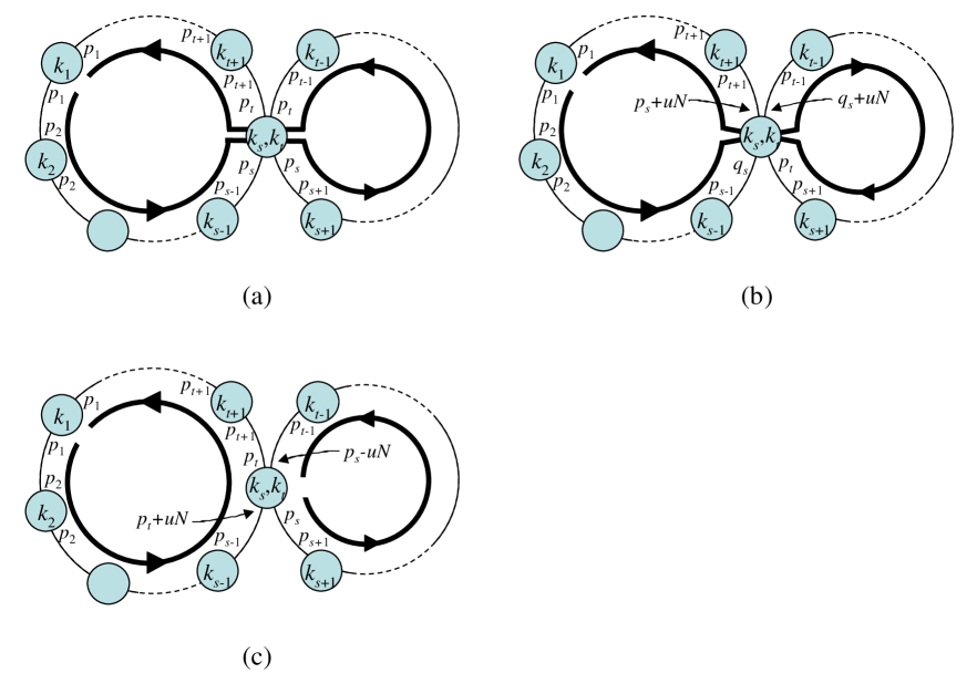
Figure 7: The directed flows represented by thick lines in (a), (b) and (c) denote the product of $\delta$ functions corresponding to the equivalence patterns of i) $q_{s}=p_{s}$ and $q_{t}=p_{t}$, ii) $p_{t}=p_{s}+uN$ and $q_{t}=q_{s}+uN$ and iii) $q_{s}=p_{t}+uN$ and $q_{t}=p_{s}-uN$, respectively.

We are going to demonstrate that, concerned with the four edge variables $p_{s},q_{s},p_{t},q_{t}$ of the merged vertex in Fig. 6(b), it is sufficient to consider $p_{t}=q_{s}$ and $p_{s}=q_{t}$. Since $k_{i}$’s are all distinct except for $k_{s}=k_{t}$, to yield a nonzero expectation of $\prod_{r=1}^{n}c_{k_{r}}^{(q_{r})}c_{k_{r}}^{(p_{r})}$ in (67) and (68), it is required that $p_{r}=q_{r}$ for $r\in\{1,2,\cdots,n\}\setminus\{s,t\}$ and $c_{k_{s}}^{(p_{s})},c_{k_{s}}^{(q_{s})},c_{k_{s}}^{(p_{t})},c_{k_{s}}^{(q_{t})}$ are in pairs, i.e., anyone of the following three conditions

1. $q_{s}=p_{s}$ and $q_{t}=p_{t}$,

2. $p_{t}=p_{s}+uN$ and $q_{t}=q_{s}+uN$ with any integer $u$,

3. $q_{s}=p_{t}+uN$ and $q_{t}=p_{s}-uN$ with any integer $u$,

for a short-code system, and

1. $q_{s}=p_{s}$ and $q_{t}=p_{t}$,

2. $p_{t}=p_{s}$ and $q_{t}=q_{s}$,

3. $q_{s}=p_{t}$ and $q_{t}=p_{s}$,

for a long-code system. The reasons for same sign of two $uN$ in condition ii) and opposite signs in condition iii) is because $m_{s}N\leq p_{s},q_{s}\leq(m_{s}+1)N-1$ and $m_{t}N\leq p_{t},q_{t}\leq(m_{t}+1)N-1$. As conditions iv)–vi) are special cases of i)–iii) with $u=0$, we will use the latter to demonstrate our goal, i.e., it is sufficient to consider only the equivalence relation of case vi).

With conditions i)–iii) and $p_{r}=q_{r}$ for $r\in\{1,2,\cdots,n\}\setminus\{s,t\}$, the contribution of each element of ${\cal X}_{n-1}(e,n-e)$ to (67) and (68) becomes

$$N^{-n+2}\lim_{M\rightarrow\infty}(2M+1)^{-1}\sum_{{\cal M}\in{\cal Y}}\sum_{p_{1}\in{\cal Z}^{\prime}_{1}}\sum_{p_{2}\in{\cal Z}^{\prime}_{2}}\cdots\sum_{p_{n}\in{\cal Z}^{\prime}_{n}}\textrm{E}\left\{c_{k_{s}}^{(p_{s})}c_{k_{s}}^{(q_{s})}c_{k_{s}}^{(p_{t})}c_{k_{s}}^{(q_{t})}\right\}$$

$$\times\delta(p_{1}T_{c}+\tau_{k_{1}},p_{2}T_{c}+\tau_{k_{2}})\delta(p_{2}T_{c}+\tau_{k_{2}},p_{3}T_{c}+\tau_{k_{3}})\cdots\delta(p_{n}T_{c}+\tau_{k_{n}},p_{1}T_{c}+\tau_{k_{1}})|_{k_{s}=k_{t}},$$ (72)

and

$$N^{-n+2}\lim_{M\rightarrow\infty}(2M+1)^{-1}\sum_{{\cal M}\in{\cal Y}}\sum_{p_{1}\in{\cal Z}^{\prime}_{1}}\sum_{p_{2}\in{\cal Z}^{\prime}_{2}}\cdots\sum_{p_{n}\in{\cal Z}^{\prime}_{n}}\textrm{E}\left\{c_{k_{s}}^{(p_{s})}c_{k_{s}}^{(q_{s})}c_{k_{s}}^{(p_{t})}c_{k_{s}}^{(q_{t})}\right\}$$

$$\times\textrm{E}\left\{R_{\psi}((p_{1}-p_{2})T_{c}+\tau_{k_{1}}-\tau_{k_{2}})R_{\psi}((p_{2}-p_{3})T_{c}+\tau_{k_{2}}-\tau_{k_{3}})\cdots\right.$$

$$\left.\hskip 28.45274ptR_{\psi}((p_{n}-p_{1})T_{c}+\tau_{k_{n}}-\tau_{k_{1}})\right\}|_{k_{s}=k_{t}},$$ (73)

respectively. A careful inspection reveals that the product of $\delta$ functions in (72) becomes

$$\mathop{\prod_{(\gamma,\epsilon)\in{\cal I}_{1}}}_{k_{t}=k_{s}}\delta(p_{\gamma}T_{c}+\tau_{k_{\gamma}},p_{\epsilon}T_{c}+\tau_{k_{\epsilon}}),\quad{\cal I}_{1}=\{(1,2),(2,3),\cdots,(n-1,n),(n,1)\}$$ (74)

for condition i), where we let $q_{s}:=p_{s}$ and $q_{t}:=p_{t}$,

$$\delta(p_{s-1}T_{c}+\tau_{k_{s-1}},q_{s}T_{c}+\tau_{k_{s}})\delta((q_{s}+uN)T_{c}+\tau_{k_{s}},p_{t-1}T_{c}+\tau_{k_{t-1}})$$

$$\hskip 28.45274pt\times\delta((p_{s}+uN)T_{c}+\tau_{k_{s}},p_{t+1}T_{c}+\tau_{k_{t+1}})\prod_{(\gamma,\epsilon)\in{\cal I}_{2}}\delta(p_{\gamma}T_{c}+\tau_{k_{\gamma}},p_{\epsilon}T_{c}+\tau_{k_{\epsilon}}),$$

$${\cal I}_{2}=\{(1,2),\cdots,(s-2,s-1),(t+1,t+2),\cdots,(n,1)\}$$

$$\hskip 56.9055pt\cup\{(s,s+1),(s+1,s+2),\cdots,(t-2,t-1)\}$$ (75)

for condition ii), where we let $p_{t}:=p_{s}+uN$ and $q_{t}:=q_{s}+uN$, and

$$\delta(p_{s-1}T_{c}+\tau_{k_{s-1}},(p_{t}+uN)T_{c}+\tau_{k_{s}})\delta(p_{t-1}T_{c}+\tau_{k_{t-1}},(p_{s}-uN)T_{c}+\tau_{k_{s}})$$

$$\hskip 28.45274pt\times\mathop{\prod_{(\gamma,\epsilon)\in{\cal I}_{3}}}_{k_{t}=k_{s}}\delta(p_{\gamma}T_{c}+\tau_{k_{\gamma}},p_{\epsilon}T_{c}+\tau_{k_{\epsilon}})\prod_{(\eta,\zeta)\in{\cal I}_{4}}\delta(p_{\eta}T_{c}+\tau_{k_{\eta}},p_{\zeta}T_{c}+\tau_{k_{\zeta}}),$$

$${\cal I}_{3}=\{(1,2),\cdots,(s-2,s-1),(t,t+1),\cdots,(n,1)\},$$

$${\cal I}_{4}=\{(s,s+1),\cdots,(t-2,t-1)\}$$ (76)

for condition iii), where $q_{s}:=p_{t}+uN$ and $q_{t}:=p_{s}-uN$. The product of $R_{\psi}$ functions in (73) can be obtained from the above equations by replacing each $\delta(a,b)$ with $R_{\psi}(a-b)$. According to (74)–(76), conditions i)–iii) are graphically represented by Figs. 7(a)–(c), respectively. For instance, in Fig. 7(a), except for the merged vertex, two edge variables touching the same vertex are the same. This is because $p_{r}=q_{r}$ for $r\in\{1,2,\cdots,n\}\setminus\{s,t\}$, so we replace $q_{r},r\in\{1,2,\cdots,n\}\setminus\{s,t\}$ in Fig. 6(b) with $p_{r}$. Moreover, $q_{s}$ and $q_{t}$ in Fig. 6(b) are replaced with $p_{s}$ and $p_{t}$, respectively, indicating that $q_{s}:=p_{s}$ and $q_{t}:=p_{t}$. In each of Figs. 7(a)–(c), the product of $\delta$ and $R_{\psi}$ functions in (72) and (73), respectively, are depicted in the form of directed flow(s), indicated by thick lines traversing edges. The thick line passing through an edge with variables $p_{\gamma}$ and $p_{\epsilon}$ (or $q_{\epsilon}$) represents $\delta(p_{\gamma}T_{c}+\tau_{k_{\gamma}},p_{\epsilon}T_{c}+\tau_{k_{\epsilon}})$ (or $\delta(p_{\gamma}T_{c}+\tau_{k_{\gamma}},q_{\epsilon}T_{c}+\tau_{k_{\epsilon}})$) for (72) and $R_{\psi}((p_{\gamma}-p_{\epsilon})T_{c}+\tau_{k_{\gamma}}-\tau_{k_{\epsilon}})$ (or $R_{\psi}((p_{\gamma}-q_{\epsilon})T_{c}+\tau_{k_{\gamma}}-\tau_{k_{\epsilon}})$) for (73). For an edge with variables $p_{\gamma}+uN$ and $p_{\epsilon}$, it corresponds to $\delta((p_{\gamma}+uN)T_{c}+\tau_{k_{\gamma}},p_{\epsilon}T_{c}+\tau_{k_{\epsilon}})$ for (72). Conditions i)–iii) are taken into account below.

• Condition i): Consider the chip-synchronous case. The product of $\delta$ functions in (74) is zero if $p_{s}\neq p_{t}$. Thus, we consider $p_{s}=p_{t}$, resulting in $p_{s}=q_{s}=p_{t}=q_{t}$, and the expectation in the first line of (72) is $O(N^{-2})$ because the fourth moment of $c_{k}^{(p)}$ is $O(N^{-2})$. It can be taken out from multi-dimensional summation, yielding

  $$O(N^{-n})\lim_{M\rightarrow\infty}(2M+1)^{-1}\sum_{{\cal M}\in{\cal Y}}\sum_{p_{1}\in{\cal Z}^{\prime}_{1}}\sum_{p_{2}\in{\cal Z}^{\prime}_{2}}\cdots\sum_{p_{n}\in{\cal Z}^{\prime}_{n}}\delta(p_{1}T_{c}+\tau_{k_{1}},p_{2}T_{c}+\tau_{k_{2}})$$

  $$\times\delta(p_{2}T_{c}+\tau_{k_{2}},p_{3}T_{c}+\tau_{k_{3}})\cdots\delta(p_{n}T_{c}+\tau_{k_{n}},p_{1}T_{c}+\tau_{k_{1}})|_{k_{s}=k_{t}}.$$ (77)

  It is readily seen that, in (77), the term behind $O(N^{-n})$ is equal to $N$. Thus, in this condition, the contribution of each element in ${\cal X}_{n-1}(e,n-e)$ to (67) is $O(N^{-n+1})$.

  Consider the case of chip-asynchronous. Assume $p_{s}\neq p_{t}$. We replace each $\delta(a,b)$ in (74) with $R_{\psi}(a-b)$ and plug the resulting product of $R_{\psi}$ functions back into (73). The expectation of chips in (73) is $N^{-2}$, and it can be taken out from the multi-sum, resulting in

  $$N^{-n}\lim_{M\rightarrow\infty}(2M+1)^{-1}\sum_{{\cal M}\in{\cal Y}}\sum_{p_{1}\in{\cal Z}^{\prime}_{1}}\sum_{p_{2}\in{\cal Z}^{\prime}_{2}}\cdots\sum_{p_{n}\in{\cal Z}^{\prime}_{n}}\textrm{E}\left\{R_{\psi}((p_{1}-p_{2})T_{c}+\tau_{k_{1}}-\tau_{k_{2}})\right.$$

  $$\hskip 28.45274pt\times\left.R_{\psi}((p_{2}-p_{3})T_{c}+\tau_{k_{2}}-\tau_{k_{3}})\cdots R_{\psi}((p_{n}-p_{1})T_{c}+\tau_{k_{n}}-\tau_{k_{1}})\right\}|_{k_{s}=k_{t}}.$$ (78)

  By Lemma 4, the term behind $N^{-n}$ is equal to $N{\cal W}_{\psi}^{(n)}$ for bandwidth of $\psi(t)$ either smaller or wider than $1/(2T_{c})$. Thus, (78) is equal to $N^{-n+1}{\cal W}_{\psi}^{(n)}$. When $p_{s}=p_{t}$, the expectation of chips in (73) is $O(N^{-2})$, and (78) is revised by changing $N^{-n}$ to $O(N^{-n})$ and imposing a constraint of $p_{s}=p_{t}$. Under these circumstances, the revised equation is equal to $O(N^{-n+1})$. Thus, with both $p_{s}=p_{t}$ and $p_{s}\neq p_{t}$, the contribution of each element of ${\cal X}_{n-1}(e,n-e)$ to (68) is $O(N^{-n+1})$.

• Condition ii): Consider the chip-synchronous case. The product of $\delta$ functions is given by (75). It can be checked that the product is zero if either $u\neq 0$ or $p_{s}\neq q_{s}$ not satisfied. Thus, we let $u=0$ and $p_{s}=q_{s}$, which yields $p_{s}=q_{s}=p_{t}=q_{t}$. By similar arguments as in condition i), the contribution of each element of ${\cal X}_{n-1}(e,n-e)$ to (67) is $O(N^{-n+1})$.

  In the case of chip-asynchronous, we replace each $\delta(a,b)$ in (75) with $R_{\psi}(a-b)$ and plug the resulting product of $R_{\psi}$ functions back into (73). For either $p_{s}=q_{s}$ or $p_{s}\neq q_{s}$, the expectation of chips in (73) is $O(N^{-2})$, and we take it out from the multi-sum. Thus the leading term in (73) becomes $O(N^{-n})$. Tracing the proof of Lemma 4, we can find that the limiting normalized infinite sum of products of $R_{\psi}$ functions in (73), i.e., the term behind the leading term, is equal to

  $$\frac{N}{2\pi T_{c}^{n-1}}\int e^{-j2uNT_{c}\Omega}\left|\Psi(\Omega)\right|^{2n}\textrm{d}\Omega.$$

  When $N$ is large, the integral is nonzero (equal to $2\pi T_{c}^{n-1}{\cal W}_{\psi}^{(n)}$) only if $u=0$. Thus, the contribution of each element of ${\cal X}_{n-1}(e,n-e)$ to (68) is $O(N^{-n+1})$.

• Condition iii): In chip-synchronous case, the product of $\delta$ functions is given by (76). This product is zero if $u\neq 0$. Thus, we consider $u=0$ and $q_{s}=p_{t}\neq q_{t}=p_{s}$, which implies $m_{s}=m_{t}$, and (72) becomes

  $$N^{-n}\lim_{M\rightarrow\infty}(2M+1)^{-1}\mathop{\sum_{m_{1},\cdots,m_{s-1},m_{t},m_{t+1},\cdots,m_{n}}}_{p_{1},\cdots,p_{s-1},p_{t},p_{t+1},\cdots,p_{n}}\mathop{\prod_{(\gamma,\epsilon)\in{\cal I}_{3}}}_{k_{t}=k_{s}}\delta(p_{\gamma}T_{c}+\tau_{k_{\gamma}},p_{\epsilon}T_{c}+\tau_{k_{\epsilon}})$$

  $$\times\mathop{\mathop{\sum_{m_{s},m_{s+1},\cdots,m_{t-1}}}_{p_{s},p_{s+1},\cdots,p_{t-1}}}_{m_{s}=m_{t}}\prod_{(\eta,\zeta)\in{\cal I}_{4}}\delta(p_{\eta}T_{c}+\tau_{k_{\eta}},p_{\zeta}T_{c}+\tau_{k_{\zeta}}).$$ (79)

  Note that, for any particular $m_{t}$, the constraint of $m_{s}=m_{t}$ results in only $N$ choices for $p_{s}\in[m_{t}N,(m_{t}+1)N-1]$ in the second line of (79). It follows that (79) is equal to $N^{-n+2}$.

  In the case of chip-asynchronous, (73) now becomes

  $$N^{-n}\lim_{M\rightarrow\infty}(2M+1)^{-1}\textrm{E}\Biggl{\{}$$

  $$\mathop{\sum_{m_{1},\cdots,m_{s-1},m_{t},m_{t+1},\cdots,m_{n}}}_{p_{1},\cdots,p_{s-1},p_{t},p_{t+1},\cdots,p_{n}}R_{\psi}((p_{s-1}-p_{t}-uN)T_{c}+\tau_{k_{s-1}}-\tau_{k_{s}})\mathop{\prod_{(\gamma,\epsilon)\in{\cal I}_{3}}}_{k_{t}=k_{s}}R_{\psi}((p_{\gamma}-p_{\epsilon})T_{c}+\tau_{k_{\gamma}}-\tau_{k_{\epsilon}})$$

  $$\mathop{\mathop{\sum_{m_{s},m_{s+1},\cdots,m_{t-1}}}_{p_{s},p_{s+1},\cdots,p_{t-1}}}_{m_{s}=m_{t}}R_{\psi}((p_{t-1}-p_{s}+uN)T_{c}+\tau_{k_{t-1}}-\tau_{k_{s}})\prod_{(\eta,\zeta)\in{\cal I}_{4}}R_{\psi}((p_{\eta}-p_{\zeta})T_{c}+\tau_{k_{\eta}}-\tau_{k_{\zeta}})\Biggr{\}}.$$ (80)

  If the sinc chip waveform is employed, the expectation of (80) can be removed. By similar arguments as in condition ii), the infinite sums in the second and third lines of (80) are zero if $u\neq 0$. By part 1) of Lemma 4, when $u=0$, (80) is equal to $N^{-n}\cdot N{\cal W}_{\psi}^{(e)}\cdot N{\cal W}_{\psi}^{(n-e)}=N^{-n+2}{\cal W}_{\psi}^{(e)}{\cal W}_{\psi}^{(n-e)}$. When the bandwidth of $\psi(t)$ is wider than $1/(2T_{c})$, the calculation is more involved. We also let $u=0$. Note that, in (80), both the product of $R_{\psi}$ functions in the second and third lines contain $\tau_{k_{s}}$. We can rewrite the equation by

  $$N^{-n}\lim_{M\rightarrow\infty}(2M+1)^{-1}$$

  $$\times\textrm{E}_{\tau_{k_{s}}}\Biggl{\{}\mathop{\sum_{m_{1},\cdots,m_{s-1},m_{t},m_{t+1},\cdots,m_{n}}}_{p_{1},\cdots,p_{s-1},p_{t},p_{t+1},\cdots,p_{n}}\textrm{E}\Biggl{\{}\mathop{\prod_{(\gamma,\epsilon)\in{\cal I}^{\prime}_{3}}}_{k_{t}=k_{s}}R_{\psi}((p_{\gamma}-p_{\epsilon})T_{c}+\tau_{k_{\gamma}}-\tau_{k_{\epsilon}})\Bigr{|}\tau_{k_{s}}\Biggr{\}}$$

  $$\hskip 42.67912pt\times\mathop{\mathop{\sum_{m_{s},m_{s+1},\cdots,m_{t-1}}}_{p_{s},p_{s+1},\cdots,p_{t-1}}}_{m_{s}=m_{t}}\textrm{E}\Biggl{\{}\Biggl{.}\prod_{(\eta,\zeta)\in{\cal I}^{\prime}_{4}}R_{\psi}((p_{\eta}-p_{\zeta})T_{c}+\tau_{k_{\eta}}-\tau_{k_{\zeta}})\Bigr{|}\tau_{k_{s}}\Biggr{\}}\Biggr{\}},$$ (81)

  where ${\cal I}^{\prime}_{3}={\cal I}_{3}\cup\{(s-1,t)\}$, ${\cal I}^{\prime}_{4}={\cal I}_{4}\cup\{(t-1,s)\}$, the first expectation at the second line is w.r.t. $\tau_{k_{s}}$, and the remaining two are w.r.t. $\{\tau_{k_{i}}\}_{i=1}^{n}$ conditioned on $\tau_{k_{s}}$. By part 2) of Lemma 4, the two inner conditional expectations in the second and third lines of (81) are equal to $N{\cal W}_{\psi}^{(e)}$ and $N{\cal W}_{\psi}^{(n-e)}$, respectively. Thus, identical to the situation when $\psi(t)$ is the sinc, the contribution of each element in ${\cal X}_{n-1}(e,n-e)$ to (68) is equal to $N^{-n+2}{\cal W}_{\psi}^{(e)}{\cal W}_{\psi}^{(n-e)}$.

To sum up, when $j=n-1$, the contributions of each element in ${\cal X}_{j}(e,n-e)$ to (67) are $O(N^{-n+1})$, $O(N^{-n+1})$, and $N^{-n+2}$ for conditions i)–iii), respectively. Regarding the contributions to (68), conditions i)–iii) have $O(N^{-n+1})$, $O(N^{-n+1})$, and $N^{-n+2}{\cal W}_{\psi}^{(e)}{\cal W}_{\psi}^{(n-e)}$, respectively. Thus, as $N\rightarrow\infty$, it is sufficient to consider condition iii) since the corresponding contribution has the highest order of $N$. Note that we require $u=0$ to get the result.

We reach the conclusion that, when $j=n-1$ with $k_{s}$ and $k_{t}$ partitioned in the same class, the equivalence conditions of edge variables $\{p_{r},q_{r}\}$ are that $p_{r}=q_{r}$ for $r\in\{1,2,\cdots,n\}\setminus\{s,t\}$, $q_{s}=p_{t}$, and $p_{s}=q_{t}$. Observing Fig. 6(b), we find that the equivalence relation can be stated as: within each of the two cycles in the $K$-graph, two edge variables touching the same vertex are equal.

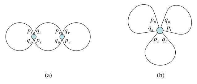
Figure 8: The $K$-graphs of $(n-2)$-class noncrossing partitions of the totally ordered set ${\cal K}=\{k_{1},k_{2},\cdots,k_{n}\}$: (a) $k_{s},k_{t}$ and $k_{u},k_{v}$ ($1\leq s<u<v<t\leq n$) are respectively in the same class and all other elements in $\cal K$ are singletons, and (b) $k_{s},k_{t},k_{u}$ are in the same class and all others are singletons.

We consider $j=n-2$ below. Two cases are possible. One is that $k_{s},k_{t}$ and $k_{u},k_{v}$ are respectively in the same class ($1\leq s<u<v<t\leq n$) and all others are singletons, whose corresponding $K$-graph is shown in Fig. 8(a). The other is that, except that $k_{s},k_{t}$ and $k_{u}$ ($s<t<u$) are partitioned in the same class, all others are singletons, whose $K$-graph is given in Fig. 8(b). In Fig. 8(a), the edge variables $p_{s},q_{s},p_{t},q_{t}$ should be paired, and so do $p_{u},q_{u},p_{v},q_{v}$. By similar arguments demonstrated above for the case of $j=n-1$, we can see the equivalence relations of $p_{t}=q_{s}$, $p_{s}=q_{t}$, $p_{v}=q_{u}$ and $p_{u}=q_{v}$ yield a contribution to (67) and (68) with the highest order of $N$. On the other hand, in Fig. 8(b), the six edge variables $p_{s},q_{s},p_{t},q_{t},p_{u},q_{v}$ should be in pairs, and the equivalence relations of $p_{s}=q_{t}$, $p_{t}=q_{u}$ and $p_{u}=q_{s}$ yield a highest order of $N$ in contribution.

From the discussions about $n-2\leq j\leq n$, the following rule can be drawn. Let $\{G_{j}\}$ denote the set of all $K$-graphs corresponding to $j$-class noncrossing partitions of ${\cal K}=\{k_{1},k_{2},\cdots,k_{n}\}$. From the noncrossing condition, it is immediate that, for any particular $\bar{G}_{j}$ in $\{G_{j}\}$, we can always find a member $\bar{G}_{j+1}$ in $\{G_{j+1}\}$ such that $\bar{G}_{j}$ is obtained from $\bar{G}_{j+1}$ by merging two vertices in the same cycle of $\bar{G}_{j+1}$. When the two vertices are merged, the cycle where these two vertices originally locate is torn into two. Within each of the two newly formed cycles, to yield a highest order of $N$ in the contribution to (67) and (68), edge variables touching the same vertex should be set to equal. This observation leads to the following lemma.

Lemma 6

Given non-ascending ordered natural numbers $b_{1},b_{2},\cdots,b_{n-j+1}$ such that $b_{1}+b_{2}+\cdots+b_{n-j+1}=n$. Suppose that $x\in{\cal X}_{j}(b_{1},b_{2},\cdots,b_{n-j+1})$. Let $G(x)$ denote the corresponding $K$-graph of $x$, and $c_{1}(x)$ and $c_{2}(x)$ stand for the contributions of $x$ to (67) and (68), respectively. To yield a highest order of $N$ in $c_{1}(x)$ and $c_{2}(x)$, in every cycle of $G(x)$, edge variables touching the same vertex should take the same value in $[1,N]$. Moreover, we have

$$c_{1}(x)=N^{-j+1}+O(N^{-j})\qquad\mbox{and}\qquad c_{2}(x)=N^{-j+1}\prod_{r=1}^{n-j+1}{\cal W}_{\psi}^{(b_{r})}+O(N^{-j}).$$

Proof:

The first part of the lemma can be proved by mathematical induction on $j$ using the observation stated in the paragraph preceding this lemma. To prove the highest-order term in $c_{1}(x)$ is $N^{-j+1}$, we note that the expectation of $\prod_{r=1}^{n}c_{k_{r}}^{(q_{r})}c_{k_{r}}^{(p_{r})}$ in (67) and (68) is equal to $N^{-n}$ when the equivalence relations of edge variables are satisfied. We take this $N^{-n}$out from the infinite sum. The limiting infinite sum of products of $\delta$ functions in (67) can be decomposed into a product of smaller limiting infinite sum of products with each corresponding to a cycle in $G(x)$ (see (79) as an example), and each decomposed limiting sum of products has a contribution of $N$ to (67). Since the number of cycles in $G(x)$ is $n-j+1$, the term with the highest order of $N$ in $c_{1}(x)$ is $N^{-n}\prod_{r=1}^{n-j+1}N=N^{-j+1}$. The proof that the highest-order term in $c_{2}(x)$ is $N^{-j+1}\prod_{r=1}^{n-j+1}{\cal W}_{\psi}^{(b_{r})}$ follows trivially from that for $c_{1}(x)$. ∎

By Lemma 6, each element of ${\cal X}_{j}(b_{1},b_{2},\cdots,b_{n-j+1})$ has the same contribution of $N^{-j+1}+O(N^{-j})$ to (67). Thus, the total contribution of ${\cal X}_{j}(b_{1},b_{2},\cdots,b_{n-j+1})$ is equal to

$$\#{\cal X}_{j}(b_{1},b_{2},\cdots,b_{n-j+1})\cdot(N^{-j+1}+O(N^{-j}))$$

$$= \frac{n(n-1)\cdots(j+1)}{f(b_{1},b_{2},\cdots,b_{n-j+1})}\prod_{r=0}^{j-1}(K-r)\cdot(N^{-j+1}+O(N^{-j})).$$

Hence, by (65), the total contribution of noncrossing partitions of $\cal K$ to $\mu({\boldsymbol{R}}_{\textrm{cs}}^{n})$ is

$$\mathop{\lim_{K,N\rightarrow\infty}}_{K/N\rightarrow\beta}K^{-1}\sum_{j=1}^{n}\hskip 5.69054pt\mathop{\sum_{b_{1}+b_{2}+\cdots+b_{n-j+1}=n}}_{b_{1}\geq b_{2}\geq\cdots\geq b_{n-j+1}\geq 1}\frac{n(n-1)\cdots(j+1)}{f(b_{1},b_{2},\cdots,b_{n-j+1})}\prod_{r=0}^{j-1}(K-r)\cdot(N^{-j+1}+O(N^{-j}))$$ (82)

$$= \dfrac{1}{n}\sum_{j=1}^{n}{n\choose j}{n\choose j-1}\beta^{j-1},$$

where the equality holds by applying change of variables to (63). Similarly, the contribution of noncrossing partitions of $\cal K$ to $\mu({\boldsymbol{R}}_{\textrm{ca}}^{n})$ is given by

$$\mathop{\lim_{K,N\rightarrow\infty}}_{K/N\rightarrow\beta}K^{-1}\sum_{j=1}^{n}\hskip 5.69054pt\mathop{\sum_{b_{1}+b_{2}+\cdots+b_{n-j+1}=n}}_{b_{1}\geq b_{2}\geq\cdots\geq b_{n-j+1}\geq 1}\frac{n(n-1)\cdots(j+1)}{f(b_{1},b_{2},\cdots,b_{n-j+1})}\prod_{r=0}^{j-1}(K-r)\cdot N^{-j+1}\prod_{s=1}^{n-j+1}{\cal W}_{\psi}^{(b_{s})}$$ (83)

$$= \sum_{j=1}^{n}\beta^{j-1}\mathop{\sum_{b_{1}+b_{2}+\cdots+b_{n-j+1}=n}}_{b_{1}\geq b_{2}\geq\cdots\geq b_{n-j+1}\geq 1}\frac{n(n-1)\cdots(j+1)}{f(b_{1},b_{2},\cdots,b_{n-j+1})}\prod_{r=1}^{n-j+1}{\cal W}_{\psi}^{(b_{r})}.$$

B-B Contributions of Crossing Partitions to $\mu({\boldsymbol{R}}_{\textrm{cs}}^{n})$ and $\mu({\boldsymbol{R}}_{\textrm{ca}}^{n})$

Let $G$ be a $K$-graph resulting from a crossing partition of $\cal K$ into $j$ classes. The graph $G$ can be decomposed into at most $n-j$ cycles. For example, Fig. 5(c) can be decomposed into at most five cycles. Thus, the contribution of $G$ to (67) is $O(N^{-n}\cdot N^{n-j})\prod_{r=0}^{j-1}(K-r)=O(1)$. By (65), the contribution of crossing partitions of $\cal K$ to $\mu({\boldsymbol{R}}_{\textrm{cs}}^{n})$ is

$$\mathop{\lim_{K,N\rightarrow\infty}}_{K/N\rightarrow\beta}K^{-1}\sum_{j=1}^{n}\#{\cal X}_{cro}(j)\cdot O(1)=0,$$ (84)

where $\#{\cal X}_{cro}(j)$ denote the number of $j$-class crossing partitions. By (82) and (84), we complete the proof of Lemma 1. Similarly, it can be shown that the contribution of crossing partitions of $\cal K$ to $\mu({\boldsymbol{R}}_{\textrm{ca}}^{n})$ vanishes in the large system limit. Thus, we have shown $\mu({\boldsymbol{R}}_{\textrm{ca}}^{n})$ is given by (83), which completes the proof for Lemma 5.

Appendix C Proof of Lemma 2

By (19), the $n$-th moment of the ESD of ${\boldsymbol{R}}_{\textrm{cs}}^{(K)}$ when $M\rightarrow\infty$ can be represented by a normalized trace operator, given as

$$\overline{\textrm{tr}}((\boldsymbol{R}_{\textrm{cs}}^{(K)})^{n})=\lim_{M\rightarrow\infty}(2M+1)^{-1}K^{-1}\operatorname{tr}((\boldsymbol{R}_{\textrm{cs}}^{(K)})^{n}).$$

Define

$$v_{K}=\overline{\textrm{tr}}((\boldsymbol{R}_{\textrm{cs}}^{(K)})^{n})-\mu({\boldsymbol{R}}_{\textrm{cs}}^{n}).$$

By Borell-Cantelli lemma [48], if

$$\sum_{K=1}^{\infty}\textrm{Prob}(|v_{K}|>\epsilon)<\infty,\qquad\forall\epsilon>0,$$

then $v_{K}\rightarrow 0$ in a.s. sense. Using Markov inequality that

$$\textrm{Prob}(|v_{K}|>\epsilon)=\textrm{Prob}(v_{K}^{2}>\epsilon^{2})\leq\textrm{E}\{v_{K}^{2}\}/\epsilon^{2},\qquad\forall\epsilon>0,$$

we can show the a.s. convergence of $v_{K}$ to 0 by proving $\sum_{K=1}^{\infty}\textrm{E}\left\{v_{K}^{2}\right\}<\infty$. In the following, we will show that

$$\sum_{K=1}^{\infty}\textrm{E}\left\{\left[\overline{\textrm{tr}}((\boldsymbol{R}_{\textrm{cs}}^{(K)})^{n})-\mu(\boldsymbol{R}_{\textrm{cs}}^{n})\right]^{2}\right\}<\infty$$ (85)

for all $n\in\mathbb{N}$, and the superscript of ${\boldsymbol{R}}_{\textrm{cs}}^{(K)}$ will be omitted for simplicity. In the proof, for simplicity, we suppose that the spreading sequences are independent from users to users, and for a particular user, the sequence is independent across symbols. That is, a long-code system is assumed. However, by following similar arguments of the proofs in Appendix B, it is straightforward to extend the proof here to a short-code system.

We have

$$\textrm{E}\left\{\left[\overline{\textrm{tr}}(\boldsymbol{R}_{\textrm{cs}}^{n})-\mu(\boldsymbol{R}_{\textrm{cs}}^{n})\right]^{2}\right\}$$ (86)

$$= \textrm{E}\left\{\left[\overline{\textrm{tr}}(\boldsymbol{R}_{\textrm{cs}}^{n})\right]^{2}\right\}-[\mu(\boldsymbol{R}_{\textrm{cs}}^{n})]^{2}$$

$$= \lim_{M\rightarrow\infty}(2M+1)^{-2}K^{-2}\sum Q(m_{1},\cdots,m_{n},m_{n+1},\cdots,m_{2n};k_{1},\cdots,k_{n},k_{n+1},\cdots,k_{2n}),$$

where

$$Q(m_{1},\cdots,m_{n},m_{n+1},\cdots,m_{2n};k_{1},\cdots,k_{n},k_{n+1},\cdots,k_{2n})$$ (88)

$$= \textrm{E}\{[\boldsymbol{R}_{\textrm{cs}}]_{m_{1}m_{2},k_{1}k_{2}}[\boldsymbol{R}_{\textrm{cs}}]_{m_{2}m_{3},k_{2}k_{3}}\cdots[\boldsymbol{R}_{\textrm{cs}}]_{m_{n}m_{1},k_{n}k_{1}}$$

$$\times[\boldsymbol{R}_{\textrm{cs}}]_{m_{n+1}m_{n+2},k_{n+1}k_{n+2}}[\boldsymbol{R}_{\textrm{cs}}]_{m_{n+2}m_{n+3},k_{n+2}k_{n+3}}\cdots[\boldsymbol{R}_{\textrm{cs}}]_{m_{2n}m_{n+1},k_{2n}k_{n+1}}\}$$

$$-\textrm{E}\{[\boldsymbol{R}_{\textrm{cs}}]_{m_{1}m_{2},k_{1}k_{2}}[\boldsymbol{R}_{\textrm{cs}}]_{m_{2}m_{3},k_{2}k_{3}}\cdots[\boldsymbol{R}_{\textrm{cs}}]_{m_{n}m_{1},k_{n}k_{1}}\}$$

$$\times\textrm{E}\{[\boldsymbol{R}_{\textrm{cs}}]_{m_{n+1}m_{n+2},k_{n+1}k_{n+2}}[\boldsymbol{R}_{\textrm{cs}}]_{m_{n+2}m_{n+3},k_{n+2}k_{n+3}}\cdots[\boldsymbol{R}_{\textrm{cs}}]_{m_{2n}m_{n+1},k_{2n}k_{n+1}}\},$$

and the summation is over all $-M\leq m_{1},\cdots,m_{2n}\leq M$ and $1\leq k_{1},\cdots,k_{2n}\leq K$. Moreover, we have $|m_{j}-m_{j+1}|\leq 1$ for $\{m_{j}\}_{j=1}^{n}$, and so do $\{m_{j}\}_{j=n+1}^{2n}$.

We consider two $n$-element noncrossing partitions. One is for $\{k_{1},\cdots,k_{n}\}$, and the other is for $\{k_{n+1},\cdots,k_{2n}\}$. Suppose that there are $j$ and $l$ classes in the former and latter partitions, respectively. Assume $j$ classes of noncrossing partitions of $\{k_{1},\cdots,k_{n}\}$ take distinct values $\{u_{1},\cdots,u_{j}\}$ in $[1,K]$, and they have sizes $(a_{1},\cdots,a_{j})$, respectively. Similarly, $\{k_{n+1},\cdots,k_{2n}\}$ take values $\{v_{1},\cdots,v_{l}\}$, which have sizes $(b_{1},\cdots,b_{l})$, respectively.

First, consider the case that $\{u_{1},\cdots,u_{j}\}$ and $\{v_{1},\cdots,v_{l}\}$ have no common element, i.e., all of $u_{1},\cdots,u_{j},v_{1},\cdots,v_{l}$ are distinct. Due to independence of spreading codes $c_{k}^{(p)}$’s, the first term of (88) (expectation of a product of $2n$ elements) is equal to the second term. Thus, $Q(m_{1},\cdots,m_{n},$ $m_{n+1},\cdots,m_{2n};k_{1},\cdots,k_{n},k_{n+1},\cdots,k_{2n})$ is equal to zero, and (85) follows trivially.

Secondly, consider the situation that $\{u_{1},\cdots,u_{j}\}$ and $\{v_{1},\cdots,v_{l}\}$ have only one element in common. Without loss of generality, we let $u_{1}=v_{1}=w$. In this case, (88) is equal to

$$\sum\left\{\textrm{E}\left(\prod_{\alpha(1)=1}^{a_{1}}c_{w}^{(p_{1,\alpha(1)})}c_{w}^{(q_{1,\alpha(1)})}\prod_{\gamma(1)=1}^{b_{1}}c_{w}^{(r_{1,\gamma(1)})}c_{w}^{(s_{1,\gamma(1)})}\right)\right.$$ (89)

$$\hskip 28.45274pt-\left.\textrm{E}\left(\prod_{\alpha(1)=1}^{a_{1}}c_{w}^{(p_{1,\alpha(1)})}c_{w}^{(q_{1,\alpha(1)})}\right)\textrm{E}\left(\prod_{\gamma(1)=1}^{b_{1}}c_{w}^{(r_{1,\gamma(1)})}c_{w}^{(s_{1,\gamma(1)})}\right)\right\}$$

$$\times\prod_{i=2}^{j}\textrm{E}\left(\prod_{\alpha(i)=1}^{a_{i}}c_{u_{i}}^{(p_{i,\alpha(i)})}c_{u_{i}}^{(q_{i,\alpha(i)})}\right)\cdot\prod_{i=2}^{l}\textrm{E}\left(\prod_{\gamma(i)=1}^{b_{i}}c_{v_{i}}^{(r_{i,\gamma(i)})}c_{v_{i}}^{(s_{i,\gamma(i)})}\right)\times\mbox{product of $\delta$ functions},$$

where, for given $i$ and $\alpha(i)$, $p_{i,\alpha(i)}$ and $q_{i,\alpha(i)}$ are edge variables touching the same vertex within a cycle of the $K$-graph, and so do $r_{i,\gamma(i)}$ and $s_{i,\gamma(i)}$ with given $i$ and $\gamma(i)$. The summation in (89) is over all $p_{i,\alpha(i)}$, $q_{i,\alpha(i)}$, $i=1,\cdots,j$, $\alpha(i)=1,\cdots,a_{i}$ and $r_{i,\gamma(i)}$, $s_{i,\gamma(i)}$, $i=1,\cdots,l$, $\gamma(i)=1,\cdots,b_{i}$. Equation (89) is nonzero if and only if all the following conditions are met:

• for each $2\leq i\leq j$, elements in $\{p_{i,1},\cdots,p_{i,a_{i}},q_{i,1},\cdots,q_{i,a_{i}}\}$ are in pairs,

• for each $2\leq i\leq l$, elements in $\{r_{i,1},\cdots,r_{i,b_{i}},s_{i,1},\cdots,s_{i,b_{i}}\}$ are in pairs,

• elements of $\{p_{1,1},\cdots,p_{1,a_{1}},q_{1,1},\cdots,q_{1,a_{1}},r_{1,1},\cdots,r_{1,b_{1}},s_{1,1},\cdots,s_{1,b_{1}}\}$ are in pair, and some of $p_{1,1},$ $\cdots,p_{1,a_{1}},$ $q_{1,1},\cdots,q_{1,a_{1}}$ are in pair with elements of $r_{1,1},\cdots,r_{1,b_{1}},s_{1,1},\cdots,s_{1,b_{1}}$,

where we say members of a set are in pairs, if each element of the set can find odd number of other elements that take the same value. To have the largest cardinality of summation variables $m_{1},\cdots,m_{2n}$, $p_{i,\alpha(i)}$’s, $q_{i,\alpha(i)}$’s, $r_{i,\gamma(i)}$’s and $s_{i,\gamma(i)}$’s in (89), the pairing constraints listed in conditions 1)–3) above should be as least as possible, which yields

• for each $2\leq i\leq j$, $\{p_{i,1},\cdots,p_{i,a_{i}},q_{i,1},\cdots,q_{i,a_{i}}\}$ is paired by, for each $1\leq\alpha(i)\leq a_{i}$, $p_{i,\alpha(i)}$ is only paired with $q_{i,\alpha(i)}$,

• for each $2\leq i\leq l$, $\{r_{i,1},\cdots,r_{i,b_{i}},s_{i,1},\cdots,s_{i,b_{i}}\}$ is paired by, for each $1\leq\gamma(i)\leq b_{i}$, $r_{i,\gamma(i)}$ is only paired with $s_{i,\gamma(i)}$,

• there exists a unique $(\theta,\nu)\in[1,a_{1}]\times[1,b_{1}]$, denoted by $(\theta_{0},\nu_{0})$, such that $p_{1,\theta_{0}}$ is paired with $r_{1,\nu_{0}}$, and $q_{1,\theta_{0}}$ is paired with $s_{1,\nu_{0}}$ (or $p_{1,\theta_{0}}$ paired with $s_{1,\nu_{0}}$ and $q_{1,\theta_{0}}$ paired with $r_{1,\nu_{0}}$),

• for $\{p_{1,1},\cdots,p_{1,a_{1}},q_{1,1},\cdots,q_{1,a_{1}}\}$, $p_{1,\alpha(1)}$ is only paired with $q_{1,\alpha(1)}$ when $\alpha(1)\neq\theta_{0}$,

• for $\{r_{1,1},\cdots,r_{1,b_{1}},s_{1,1},\cdots,s_{1,b_{1}}\}$, $r_{1,\gamma(1)}$ is only paired with $s_{1,\gamma(1)}$ when $\gamma(1)\neq\nu_{0}$.

Under these circumstances, the summand of (89) without the product of $\delta$ functions is $O(N^{-2n})$. On the other hand, for each $m_{1}$ and $m_{n+1}$, the product of $\delta$ functions in (89) summed over dummy variables $m_{1},\cdots,m_{n},$ $m_{n+1},\cdots,m_{2n}$, $p_{i,\alpha(i)}$’s, $q_{i,\alpha(i)}$’s, $r_{i,\gamma(i)}$’s and $s_{i,\gamma(i)}$’s is

$$O(N^{n-j+1}\cdot N^{n-l+1}\cdot N^{-1})=O(N^{2n-j-l+1}),$$

where $N^{n-j+1}$ and $N^{n-l+1}$ are because $\{k_{1},\cdots,k_{n}\}$ and $\{k_{n+1},\cdots,k_{2n}\}$ form $j$- and $l$-class noncrossing partitions, respectively, and $N^{-1}$ is because conditions 6)–8) causes the cardinality reduced by one. Thus, (86) is qual to

$$K^{-2}\cdot O(N^{-2n})\cdot O(K^{j+l-1})\cdot O(N^{2n-j-l+1})=O(K^{-2}),$$ (90)

where $O(K^{j+l-1})$ is because $u_{1},\cdots,u_{j},v_{1},\cdots,v_{l}$ are all distinct except for $u_{1}=v_{1}$. Consider the infinite sum over $K$ of (85). It is finite when (90) is summed over $K$ from $1$ to $\infty$.

Next, we consider the situation that $\{u_{1},\cdots,u_{j}\}$ and $\{v_{1},\cdots,v_{l}\}$ have $t$ elements in common, where $2\leq t\leq\min(j,l)$. Without loss of generality, we assume $u_{i}=v_{i}=w_{i}$, $1\leq i\leq t$. In this case, (88) is equal to

$$\sum\left\{\prod_{i=1}^{t}\textrm{E}\left(\prod_{\alpha(i)=1}^{a_{i}}c_{w_{i}}^{(p_{i,\alpha(i)})}c_{w_{i}}^{(q_{i,\alpha(i)})}\prod_{\gamma(i)=1}^{b_{i}}c_{w_{i}}^{(r_{i,\gamma(i)})}c_{w_{i}}^{(s_{i,\gamma(i)})}\right)\right.$$ (91)

$$\left.\hskip 28.45274pt-\prod_{i=1}^{t}\textrm{E}\left(\prod_{\alpha(i)=1}^{a_{i}}c_{w_{i}}^{(p_{i,\alpha(i)})}c_{w_{i}}^{(q_{i,\alpha(i)})}\right)\textrm{E}\left(\prod_{\gamma(i)=1}^{b_{i}}c_{w_{i}}^{(r_{i,\gamma(i)})}c_{w_{i}}^{(s_{i,\gamma(i)})}\right)\right\}$$

$$\times\prod_{i=t+1}^{j}\textrm{E}\left(\prod_{\alpha(i)=1}^{a_{i}}c_{u_{i}}^{(p_{i,\alpha(i)})}c_{u_{i}}^{(q_{i,\alpha(i)})}\right)\cdot\prod_{i=t+1}^{l}\textrm{E}\left(\prod_{\gamma(i)=1}^{b_{i}}c_{v_{i}}^{(r_{i,\gamma(i)})}c_{v_{i}}^{(s_{i,\gamma(i)})}\right)\times\mbox{product of $\delta$ functions}.$$

The pairing constraints listed in 4)–8) is one of the conditions that yield (91) nonzero and have the largest cardinality of summation variables. Thus, the contribution of the sum of products of $\delta$ functions is the same as that of when $\{u_{1},\cdots,u_{j}\}$ and $\{v_{1},\cdots,v_{l}\}$ have only one common element. That is, it is equal to $O(N^{2n-j-l+1})$. It is not difficult to see, when $\{u_{1},\cdots,u_{j}\}$ and $\{v_{1},\cdots,v_{l}\}$ have $t$ common elements, the contribution to (86) is

$$K^{-2}\cdot O(N^{-2n})\cdot O(K^{j+l-t})\cdot O(N^{2n-j-l+1})=O(K^{-t-1}).$$ (92)

When (92) is summed over $K$ from 1 to $\infty$, it is finite.

Thus, we have proved

$$\sum_{K=1}^{\infty}\textrm{E}\left\{\left[\overline{\textrm{tr}}(\boldsymbol{R}_{\textrm{cs}}^{n})-\mu(\boldsymbol{R}_{\textrm{cs}}^{n})\right]^{2}\right\}<\infty$$

for all natural numbers $n$, meaning that $\overline{\textrm{tr}}(\boldsymbol{R}_{\textrm{cs}}^{n})$ converges a.s. to $\mu(\boldsymbol{R}_{\textrm{cs}}^{n})$ when $K\rightarrow\infty$. Moreover, it is seen $\mu({\boldsymbol{R}}_{\textrm{cs}}^{n})$ given in (25) is equal to the $n$-th moment of the Marc̆enko-Pastur distribution. It has been proved in [26] that the moment sequence of the distribution satisfies the Carleman’s criterion.

Appendix D Proof of Lemma 3

Let $\boldsymbol{P}=\boldsymbol{A}\boldsymbol{A}^{\dagger}$. Matrix $\boldsymbol{P}$ has the same structure as $\boldsymbol{A}$. The $k$-th diagonal entry in the $m$-th block diagonal component of $\boldsymbol{P}$ is $P_{k}(m)=|A_{k}(m)|^{2}$. We have

$$\operatorname{tr}\{(\boldsymbol{A}^{\dagger}\boldsymbol{R}_{\textrm{cs}}\boldsymbol{A})^{n}\}=\operatorname{tr}\{(\boldsymbol{R}_{\textrm{cs}}\boldsymbol{P})^{n}\},$$

and

$$\mathop{\lim_{K,N,M\rightarrow\infty}}_{K/N\rightarrow\beta}(2M+1)^{-1}K^{-1}\textrm{E}\{\operatorname{tr}((\boldsymbol{R}_{\textrm{cs}}\boldsymbol{P})^{n})\}$$ (93)

$$= \mathop{\lim_{K,N,M\rightarrow\infty}}_{K/N\rightarrow\beta}(2M+1)^{-1}K^{-1}\sum_{j=1}^{n}\mathop{\sum_{b_{1}+b_{2}+\cdots+b_{n-j+1}=n}}_{b_{1}\geq b_{2}\geq\cdots b_{n-j+1}\geq 1}\sum_{{\cal K}\in{\cal X}_{j}(b_{1},b_{2},\cdots,b_{n-j+1})}\sum_{{\cal M}\in{\cal Y}}\sum_{{\cal P}_{1}\in{\cal Z}_{1}}\cdots\sum_{{\cal P}_{n}\in{\cal Z}_{n}}$$

$$\textrm{E}\left\{\left(c_{k_{1}}^{(p_{1})}c_{k_{2}}^{(q_{2})}\right)\left(c_{k_{2}}^{(p_{2})}c_{k_{3}}^{(q_{3})}\right)\cdots\left(c_{k_{n}}^{(p_{n})}c_{k_{1}}^{(q_{1})}\right)\right\}\textrm{E}\{P_{k_{1}}(m_{1})P_{k_{2}}(m_{2})\cdots P_{k_{n}}(m_{n})\}$$

$$\times\delta(p_{1}T_{c}+\tau_{k_{1}},q_{2}T_{c}+\tau_{k_{2}})\delta(p_{2}T_{c}+\tau_{k_{2}},q_{3}T_{c}+\tau_{k_{3}})\cdots\delta(p_{n}T_{c}+\tau_{k_{n}},q_{1}T_{c}+\tau_{k_{1}}),$$

with $|m_{j}-m_{j+1}|\leq 1$. Consider the contribution of an element $x$ in ${\cal X}_{j}(b_{1},b_{2},\cdots,b_{n-j+1})$, which has a $K$-graph composed of $n-j+1$ concatenated cycles with the number of edges $b_{1},b_{2},\cdots,b_{n-j+1}$ in a non-ascending order. Suppose that this $K$-graph is yielded by a $j$-class noncrossing partition of $\cal K$ with non-ascending class sizes $(c_{1},c_{2},\cdots,c_{j})$. As shown in (64), the number of elements in ${\cal X}_{j}(b_{1},b_{2},\cdots,b_{n-j+1})$ satisfying these conditions is equal to

$$\dfrac{n(n-j)!(j-1)!}{f(b_{1},b_{2},\cdots,b_{n-j+1})f(c_{1},c_{2},\cdots,c_{j})}.$$

For $x$, the limit of the corresponding $\textrm{E}\{P_{k_{1}}(m_{1})P_{k_{2}}(m_{2})\cdots P_{k_{n}}(m_{n})\}$ in (93) becomes $\prod_{r=1}^{j}{\cal P}^{(c_{r})}$, where note that if $k_{s}$ and $k_{t}$ of $\cal K$ are partitioned in the same class, $m_{s}$ is equal to $m_{t}$. Thus, for either short-code or long-code system, (93) can be expressed as

$$\mathop{\lim_{K,N,M\rightarrow\infty}}_{K/N\rightarrow\beta}K^{-1}\sum_{j=1}^{n}\mathop{\sum_{b_{1}+b_{2}+\cdots+b_{n-j+1}=n}}_{b_{1}\geq b_{2}\geq\cdots b_{n-j+1}\geq 1}\mathop{\sum_{c_{1}+c_{2}+\cdots+c_{j}=n}}_{c_{1}\geq c_{2}\geq\cdots c_{j}\geq 1}\dfrac{n(n-j)!(j-1)!}{f(b_{1},b_{2},\cdots,b_{n-j+1})f(c_{1},c_{2},\cdots,c_{j})}$$

$$\times\prod_{s=0}^{j-1}(K-s)\cdot N^{-j+1}\cdot\prod_{r=1}^{j}{\cal P}^{(c_{r})},$$ (94)

$$=\sum_{j=1}^{n}\beta^{j-1}\mathop{\sum_{c_{1}+c_{2}+\cdots+c_{j}=n}}_{c_{1}\geq c_{2}\geq\cdots\geq c_{j}\geq 1}\dfrac{n(n-1)\cdots(n-j+2)}{f(c_{1},c_{2},\cdots,c_{j})}\prod_{r=1}^{j}{\cal P}^{(c_{r})},$$ (95)

where we make use of the equality

$$\mathop{\sum_{b_{1}+b_{2}+\cdots+b_{n-j+1}=n}}_{b_{1}\geq b_{2}\geq\cdots b_{n-j+1}\geq 1}\dfrac{n(n-j)!(j-1)!}{f(b_{1},b_{2},\cdots,b_{n-j+1})}=n(n-1)\cdots(n-j+2).$$ (96)

Appendix E Proof of Lemma 4

We prove parts 1) and 2) of this lemma in Appendices E-A and E-B, respectively.

E-A Bandwidth of $\psi(t)$ Less Than $1/(2T_{c})$

Define $\theta_{1}=n_{0}T_{c}+\eta_{0}-\eta_{1}$, $\theta_{2}=n_{2}T_{c}+\eta_{2}-\eta_{1}$, $\tilde{R}_{\psi,1}(x)=R_{\psi}(-x+\theta_{1})$, and $\tilde{R}_{\psi,2}(x)=R_{\psi}(x-\theta_{2})$. Then $R_{\psi}((n_{0}-n_{1})T_{c}+\eta_{0}-\eta_{1})$ is the sample of $\tilde{R}_{\psi,1}(x)$ at $x=n_{1}T_{c}$. The discrete-time signal $\tilde{R}_{\psi,1}(n)$ obtained from the continuous-time $\tilde{R}_{\psi,1}(x)$ by a sampling period of $T_{c}$ is denoted by the same notation, but the argument is an integer indicating the sample index.

By Parseval’s theorem, a partial sum w.r.t. $n_{1}$ in (29) can be given as

$$\sum_{n_{1}=-\infty}^{\infty}R_{\psi}((n_{0}-n_{1})T_{c}+\eta_{0}-\eta_{1})R_{\psi}((n_{1}-n_{2})T_{c}+\eta_{1}-\eta_{2})$$

$$= \sum_{n_{1}=-\infty}^{\infty}\tilde{R}_{\psi,1}(n_{1})\tilde{R}_{\psi,2}(n_{1})$$

$$= \frac{1}{2\pi}\int_{-\pi}^{\pi}\textrm{DTFT}\{\tilde{R}_{\psi,1}(n_{1})\}\textrm{DFTF}^{*}\{\tilde{R}_{\psi,2}(n_{1})\}\textrm{d}\omega,$$ (98)

where $\textrm{DTFT}\{\cdot\}$ is the operator of discrete-time Fourier transform (DTFT) with

$$\textrm{DTFT}\{x(n)\}=\sum_{n=-\infty}^{\infty}x(n)e^{-j\omega n}.$$

As $\tilde{R}_{\psi,1}(n_{1})$ is the sample of $R_{\psi}(-x+\theta_{1})$ at time $x=n_{1}T_{c}$, and the Fourier transform of $R_{\psi}(x)=\psi(x)\ast\psi(-x)$ is $|\Psi(\Omega)|^{2}$, we have

$$\textrm{DFTF}\{\tilde{R}_{\psi,1}(n_{1})\}=\dfrac{1}{T_{c}}\sum_{k=-\infty}^{\infty}e^{-j\frac{\omega-2\pi k}{T_{c}}\theta_{1}}\left|\Psi\left(\dfrac{\omega-2\pi k}{T_{c}}\right)\right|^{2},$$

where $\omega=\Omega T_{c}$. Consequently, (98) is equal to

$$\frac{1}{2\pi T_{c}^{2}}\sum_{k,l=-\infty}^{\infty}\int_{-\pi}^{\pi}e^{-j\frac{\omega-2\pi k}{T_{c}}\theta_{1}+j\frac{\omega-2\pi l}{T_{c}}\theta_{2}}\left|\Psi\left(\frac{\omega-2\pi k}{T_{c}}\right)\right|^{2}\left|\Psi\left(\frac{\omega-2\pi l}{T_{c}}\right)\right|^{2}\textrm{d}\omega,$$ (99)

where, since $\Psi(\Omega)$ is bandlimited to $\pi/T_{c}$, only $k=l=0$ has nonzero integral. Thus, (E-A) is equal to

$$\frac{1}{2\pi T_{c}^{2}}\int_{-\pi}^{\pi}e^{-j\frac{\omega}{T_{c}}((n_{0}-n_{2})T_{c}+\eta_{0}-\eta_{2})}\left|\Psi\left(\frac{\omega}{T_{c}}\right)\right|^{4}\textrm{d}\omega.$$ (100)

We consider the summation w.r.t. $n_{2}$ in (29). Define $\theta_{3}=n_{3}T_{c}+\eta_{3}-\eta_{2}$ and $\tilde{R}_{\psi,3}(x)=R_{\psi}(x-\theta_{3})$. We have

$$\sum_{n_{2}=-\infty}^{\infty}\left(\frac{1}{2\pi T_{c}^{2}}\int_{-\pi}^{\pi}e^{-j\frac{\omega}{T_{c}}((n_{0}-n_{2})T_{c}+\eta_{0}-\eta_{2})}\left|\Psi\left(\frac{\omega}{T_{c}}\right)\right|^{4}\textrm{d}\omega\right)R_{\psi}((n_{2}-n_{3})T_{c}+\eta_{2}-\eta_{3})$$ (101)

$$= \frac{1}{2\pi T_{c}^{2}}\int_{-\pi}^{\pi}e^{-j\frac{\omega}{T_{c}}(n_{0}T_{c}+\eta_{0}-\eta_{2})}\left|\Psi\left(\frac{\omega}{T_{c}}\right)\right|^{4}\left(\sum_{n_{2}=-\infty}^{\infty}e^{j\omega n_{2}}\tilde{R}_{\psi,3}(n_{2})\right)\textrm{d}\omega,$$

where the summation inside the brackets of (101) is the complex conjugate of the DTFT of $\tilde{R}_{\psi,3}(n_{2})$, given by

$$\frac{1}{T_{c}}\sum_{k=-\infty}^{\infty}e^{j\frac{\omega-2\pi k}{T_{c}}\theta_{3}}\left|\Psi\left(\frac{\omega-2\pi k}{T_{c}}\right)\right|^{2}.$$ (102)

Plugging (102) back to (101), we can see that the integral is nonzero only when $k=0$, which results in

$$\frac{1}{2\pi T_{c}^{3}}\int_{-\pi}^{\pi}e^{-j\frac{\omega}{T_{c}}((n_{0}-n_{3})T_{c}+\eta_{0}-\eta_{3})}\left|\Psi\left(\frac{\omega}{T_{c}}\right)\right|^{6}\textrm{d}\omega.$$ (103)

In consequence, when the summations w.r.t. $n_{1}$ and $n_{2}$ are taken into account, the result is given in (103). Continuing this process, we obtain the final result as

$$\frac{1}{2\pi T_{c}^{m}}\int_{-\pi}^{\pi}\left|\Psi\left(\frac{\omega}{T_{c}}\right)\right|^{2m}\textrm{d}\omega,$$

which is equal to (30) by setting $\Omega=\omega/T_{c}$.

E-B Bandwidth of $\psi(t)$ Greater Than $1/(2T_{c})$

Suppose that the bandwidth of $\psi(t)$ is greater than $\alpha/(2T_{c})$ but less than $(\alpha+1)/(2T_{c})$ for $\alpha\in\mathbb{N}$. Using the equality $\textrm{E}_{u,v}\{g(u,v)\}=\textrm{E}_{v}\{\textrm{E}_{u}\{g(u,v)|v\}\}$ with $\textrm{E}_{u}\{\cdot|\cdot\}$ denoting the conditional expectation w.r.t. $u$, we can see that

$$\sum_{n_{1}=-\infty}^{\infty}\textrm{E}_{\eta_{1}}\{R_{\psi}((n_{0}-n_{1})T_{c}+\eta_{0}-\eta_{1})R_{\psi}((n_{1}-n_{2})T_{c}+\eta_{1}-\eta_{2})|\eta_{2}\}$$ (104)

is nested in the multi-dimensional summation of (31), where note that $\eta_{0}$ is deterministic. By employing the same procedures of getting (99), it is immediate (104) becomes

$$\frac{1}{2\pi T_{c}^{2}}\sum_{k,l=-\infty}^{\infty}\int_{-\pi}^{\pi}\textrm{E}_{\eta_{1}}\left\{\left.e^{-j\frac{\omega-2\pi k}{T_{c}}\theta_{1}+j\frac{\omega-2\pi l}{T_{c}}\theta_{2}}\right|\eta_{2}\right\}\left|\Psi\left(\frac{\omega-2\pi k}{T_{c}}\right)\right|^{2}\left|\Psi\left(\frac{\omega-2\pi l}{T_{c}}\right)\right|^{2}\textrm{d}\omega,$$

whose imaginary part is definitely zero. Since $\textrm{E}_{\eta_{1}}\left\{\cos(2\pi k\eta_{1}/T_{c})\right\}=0$ for any nonzero integer $k$, it is readily seen that we only need to consider $k=l$ in the above equation, which is given by

$$\frac{1}{2\pi T_{c}^{2}}\sum_{k=-\lceil\alpha/2\rceil}^{\lceil\alpha/2\rceil}\int_{-\pi}^{\pi}e^{-j\frac{\omega-2\pi k}{T_{c}}((n_{0}-n_{2})T_{c}+\eta_{0}-\eta_{2})}\left|\Psi\left(\frac{\omega-2\pi k}{T_{c}}\right)\right|^{4}\textrm{d}\omega.$$ (105)

Consider one more layer of summations in (31), i.e., w.r.t. $n_{2}$, which yields

$$\frac{1}{2\pi T_{c}^{2}}\sum_{k=-\lceil\alpha/2\rceil}^{\lceil\alpha/2\rceil}\int_{-\pi}^{\pi}\left|\Psi\left(\frac{\omega-2\pi k}{T_{c}}\right)\right|^{4}\left(\sum_{n_{2}=-\infty}^{\infty}\textrm{E}_{\eta_{2}}\left\{\left.e^{-j\frac{\omega-2\pi k}{T_{c}}((n_{0}-n_{2})T_{c}+\eta_{0}-\eta_{2})}\tilde{R}_{\psi,3}(n_{2})\right|\eta_{3}\right\}\right)\textrm{d}\omega,$$ (106)

where the term inside the brackets can be written as

$$\textrm{E}_{\eta_{2}}\left\{\left.e^{-j\frac{\omega-2\pi k}{T_{c}}(n_{0}T_{c}+\eta_{0}-\eta_{2})}\sum_{n_{2}=-\infty}^{\infty}e^{j\omega n_{2}}\tilde{R}_{\psi,3}(n_{2})\right|\eta_{3}\right\}$$ (107)

$$= \frac{1}{T_{c}}\sum_{l=-\infty}^{\infty}\textrm{E}_{\eta_{2}}\left\{\left.e^{-j\frac{\omega-2\pi k}{T_{c}}(n_{0}T_{c}+\eta_{0}-\eta_{2})}e^{j\frac{\omega-2\pi l}{T_{c}}(n_{3}T_{c}+\eta_{3}-\eta_{2})}\right|\eta_{3}\right\}\left|\Psi\left(\frac{\omega-2\pi l}{T_{c}}\right)\right|^{2}$$

with the expectation in (107) being nonzero only when $l=k$. Thus, the summations w.r.t. $n_{1}$ and $n_{2}$ of (31), i.e., (106), become

$$\frac{1}{2\pi T_{c}^{3}}\sum_{k=-\lceil\alpha/2\rceil}^{\lceil\alpha/2\rceil}\int_{-\pi}^{\pi}e^{-j\frac{\omega-2\pi k}{T_{c}}((n_{0}-n_{3})T_{c}+\eta_{0}-\eta_{3})}\left|\Psi\left(\frac{\omega-2\pi k}{T_{c}}\right)\right|^{6}\textrm{d}\omega.$$

Continuing this process, we obtain the final result as

$$\frac{1}{2\pi T_{c}^{m}}\sum_{k=-\lceil\alpha/2\rceil}^{\lceil\alpha/2\rceil}\int_{-\pi}^{\pi}\left|\Psi\left(\frac{\omega-2\pi k}{T_{c}}\right)\right|^{2m}\textrm{d}\omega=\frac{1}{2\pi T_{c}^{m}}\int_{-(2\lceil\alpha/2\rceil+1)\pi}^{(2\lceil\alpha/2\rceil+1)\pi}\left|\Psi\left(\frac{\omega}{T_{c}}\right)\right|^{2m}\textrm{d}\omega,$$

which is equal to (32) by changing variable from $\omega$ to $\Omega=\omega/T_{c}$.

Appendix F Proof of Theorem 6

The following two lemmas are helpful to prove Theorem 6.

Lemma 7

Suppose that $\varpi$ is a noncrossing partition of a finite totally ordered set $S$, where every class in $\varpi$ has at least two elements. Then, there exist some classes in $\varpi$ that contain adjacent elements of $S$, where the adjacency is cyclic ordering, i.e., the first and last elements of $S$ are adjacent.

Proof:

Denote the $K$-graph corresponding to $\varpi$ by $G(\varpi)$. From the properties of a $K$-graph given in Appendix B, there is a bijective correspondence between the class set of $\varpi$ and the vertex set of $G(\varpi)$. We have the following three observations. First, the size of the $r$-th class of $\varpi$ is equal to $d(v_{r})/2$, where $v_{r}$ is the vertex in $G(\varpi)$ that corresponds to the $r$-th class, and $d(v_{r})$ is the degree of $v_{r}$. Secondly, whenever two adjacent elements of $S$ locate in the same class of $\varpi$, there is a self-loop in $G(\varpi)$. Thirdly, for all noncrossing partitions $\varpi$ of $S$, we cannot find any $G(\varpi)$ that contains no self-loops and whose every vertex has the degree equal to or greater than four. Based on the first two observations, the third one can be interpreted as the statement of the lemma. Thus, we have completed the proof. ∎

Lemma 8

Let ${\boldsymbol{D}}$ be the diagonal random matrix described in Theorem 6. We have, for $\textrm{x}\in\{\textrm{cs,ca}\}$,

$$\mathop{\lim_{K,N,M\rightarrow\infty}}_{K/N\rightarrow\beta}(2M+1)^{-1}K^{-1}\mathop{\sum_{{\cal K}\in{\cal X}}}_{k_{t}=k_{t+1}}\sum_{{\cal M}\in{\cal Y}}\textrm{E}\{[\boldsymbol{R}_{\textrm{x}}^{r_{1}}]_{m_{1}m_{2},k_{1}k_{2}}[\boldsymbol{D}^{s_{1}}]_{m_{2}m_{2},k_{2}k_{2}}$$ (109)

$$\hskip 28.45274pt[\boldsymbol{R}_{\textrm{x}}^{r_{2}}]_{m_{2}m_{3},k_{2}k_{3}}[\boldsymbol{D}^{s_{2}}]_{m_{3}m_{3},k_{3}k_{3}}\cdots[\boldsymbol{R}_{\textrm{x}}^{r_{n}}]_{m_{n}m_{1},k_{n}k_{1}}[\boldsymbol{D}^{s_{n}}]_{m_{1}m_{1},k_{1}k_{1}}\},$$

$$= \mu(\boldsymbol{R}_{\textrm{x}}^{r_{t}})\mathop{\lim_{K,N,M\rightarrow\infty}}_{K/N\rightarrow\beta}(2M+1)^{-1}K^{-1}\sum_{{\cal K}\setminus\{k_{t+1}\}}\sum_{{\cal M}\setminus\{m_{t+1}\}}$$

$$\hskip 14.22636pt\textrm{E}\{(d_{k_{2}}(m_{2}))^{s_{1}}\cdots(d_{k_{t-1}}(m_{t-1}))^{s_{t-2}}(d_{k_{t}}(m_{t}))^{s_{t-1}+s_{t}}(d_{k_{t+2}}(m_{t+2}))^{s_{t+1}}\cdots(d_{k_{1}}(m_{1}))^{s_{n}}\}$$

$$\hskip 14.22636pt\textrm{E}\{[\boldsymbol{R}_{\textrm{x}}^{r_{1}}]_{m_{1}m_{2},k_{1}k_{2}}\cdots[\boldsymbol{R}_{\textrm{x}}^{r_{t-1}}]_{m_{t-1}m_{t},k_{t-1}k_{t}}[\boldsymbol{R}_{\textrm{x}}^{r_{t+1}}]_{m_{t}m_{t+2},k_{t}k_{t+2}}\cdots[\boldsymbol{R}_{\textrm{x}}^{r_{n}}]_{m_{n}m_{1},k_{n}k_{1}}\},$$

where $r_{i}$’s and $s_{i}$’s are non-negative integers, notations $\cal K$, $\cal X$, $\cal M$ and $\cal Y$ have the same definitions as in (67) and (68). When ${\boldsymbol{D}}$ is set as the identity matrix and the constraint $k_{t}=k_{t+1}$ in (109) is replaced with $k_{t}=k_{u}$ for any $t<u\leq n$, (109) is equal to $\mu({\boldsymbol{R}}_{\textrm{x}}^{r_{t}+\cdots+r_{u-1}})\mu({\boldsymbol{R}}_{\textrm{x}}^{r_{1}+\cdots+r_{t-1}+r_{u}+\cdots+r_{n}})$.

Proof:

We expand the multi-sum of matrix product in (109) as

$$\mathop{\mathop{\sum_{1\leq u_{j,l(j)}\leq K,-M\leq v_{j,l(j)}\leq M}}_{1\leq j\leq n,1\leq l(j)\leq r_{j}}}_{u_{t,1}=u_{t+1}}\textrm{E}\{(d_{u_{2,1}}(v_{2,1}))^{s_{1}}(d_{u_{3,1}}(v_{3,1}))^{s_{2}}\cdots(d_{u_{1,1}}(v_{1,1}))^{s_{n}}\}$$

$$\times\textrm{E}\{\underbrace{[\boldsymbol{R}_{\textrm{x}}]_{v_{1,1}v_{1,2},u_{1,1}u_{1,2}}[\boldsymbol{R}_{\textrm{x}}]_{v_{1,2}v_{1,3},u_{1,2}u_{1,3}}\cdots[\boldsymbol{R}_{\textrm{x}}]_{v_{1,r_{1}}v_{2,1},u_{1,r_{1}}u_{2,1}}}_{[\boldsymbol{R}_{\textrm{x}}^{r_{1}}]_{m_{1}m_{2},k_{1}k_{2}}}\cdots$$

$$\cdot\underbrace{[\boldsymbol{R}_{\textrm{x}}]_{v_{n,1}v_{n,2},u_{n,1}u_{n,2}}[\boldsymbol{R}_{\textrm{x}}]_{v_{n,2}v_{n,3},u_{n,2}u_{n,3}}\cdots[\boldsymbol{R}_{\textrm{x}}]_{v_{n,r_{n}}v_{1,1},u_{n,r_{n}}u_{1,1}}}_{[\boldsymbol{R}_{\textrm{x}}^{r_{n}}]_{m_{n}m_{1},k_{n}k_{1}}}\},$$ (110)

where we let $u_{j,1}:=k_{j}$ and $v_{j,1}:=m_{j}$ for $1\leq j\leq n$. To compute (110), we consider noncrossing partitions of the ordered set $\{u_{j,l(j)}:1\leq j\leq n,1\leq l(j)\leq r_{j}\}$ with a constraint that $u_{t,1}$ and $u_{t+1,1}$ are in the same class. The ordering of the set is clear from the equation. The $K$-graphs corresponding to these noncrossing partitions can be generated by vertex mergence of a $K$-graph, called original $K$-graph, similar to the one in Fig. 6(b). In specific, consider a cycle with $r_{1}+\cdots+r_{n}$ vertices. In a counter-clockwise direction, the vertices on this cycle are ${\cal U}=\{u_{1,1},\cdots,u_{1,r_{1}},u_{2,1},\cdots,u_{2,r_{2}},\cdots,u_{n,1},\cdots,u_{n,r_{n}}\}$. The original $K$-graph is obtained by merging vertices $u_{t,1}$ and $u_{{t+1},1}$ into one vertex. Let us call the cycles at the left- and right-hand-side as $L$-cycle and $R$-cycle, respectively.

By the property of noncrossing, it is sufficient to consider only $K$-graphs obtained by executing vertex mergence individually on $L$- and $R$-cycles. That is, noncrossing partitions are performed respectively on the two ordered sets $\{u_{t,1},\cdots,u_{t,r_{t}}\}$ and ${\cal U}\setminus\{u_{t,2},\cdots,u_{t,r_{t}},u_{t+1,1}\}$. Note that the two sets have a common element $u_{t,1}$. The $K$-graphs yielded in this way give non-vanishing contributions to (109) in the large-system regime. It follows that (110) can be written as

$$\mathop{\sum_{{\cal U}\setminus\{u_{t,2},\cdots,u_{t,r_{t}},u_{t+1,1}\}}}_{{\cal V}\setminus\{v_{t,2},\cdots,v_{t,r_{t}},v_{t+1,1}\}}\textrm{E}\{(d_{u_{2,1}}(v_{2,1}))^{s_{1}}\cdots(d_{u_{{t-1},1}}(v_{{t-1},1}))^{s_{t-2}}(d_{u_{t,1}}(v_{t,1}))^{s_{t-1}+s_{t}}(d_{u_{{t+2},1}}(v_{{t+2},1}))^{s_{t+1}}$$

$$\cdots(d_{u_{1,1}}(v_{1,1}))^{s_{n}}\}\textrm{E}\{[{\boldsymbol{R}}_{\textrm{x}}^{r_{1}}]_{v_{1,1}v_{2,1},u_{1,1}u_{2,1}}\cdots[{\boldsymbol{R}}_{\textrm{x}}^{r_{t-1}}]_{v_{{t-1},1}v_{t,1},u_{{t-1},1}u_{t,1}}[{\boldsymbol{R}}_{\textrm{x}}^{r_{t+1}}]_{v_{{t},1}v_{t+2,1},u_{{t},1}u_{t+2,1}}$$

$$\cdots[{\boldsymbol{R}}_{\textrm{x}}^{r_{n}}]_{v_{n,1}v_{1,1},u_{n,1}u_{1,1}}\}\mathop{\sum_{u_{t,2},\cdots,u_{t,r_{t}}}}_{v_{t,2},\cdots,v_{t,r_{t}}}\textrm{E}\{[{\boldsymbol{R}}_{\textrm{x}}]_{v_{t,1}v_{t,2},u_{t,1}u_{t,2}}\cdots[{\boldsymbol{R}}_{\textrm{x}}]_{v_{t,r_{t}}v_{t,1},u_{t,r_{t}}u_{t,1}}\},$$ (111)

where ${\cal V}=\{v_{1,1},\cdots,v_{1,r_{1}},v_{2,1},\cdots,v_{2,r_{2}},\cdots,v_{n,1},\cdots,v_{n,r_{n}}\}$, each $[{\boldsymbol{R}}_{\textrm{x}}^{r_{i}}]_{v_{i,1}v_{i+1,1},u_{i,1}u_{i+1,1}}$ in the second and third lines is expanded as the product $[{\boldsymbol{R}}_{\textrm{x}}]_{v_{i,1}v_{i,2},u_{i,1}u_{i,2}}[{\boldsymbol{R}}_{\textrm{x}}]_{v_{i,2}v_{i,3},u_{i,2}u_{i,3}}\cdots[{\boldsymbol{R}}_{\textrm{x}}]_{v_{i,r_{i}}v_{i+1,1},u_{i,r_{1}}u_{i+1,1}}$. The integers in $[1,K]$ chosen by elements in ${\cal U}\setminus\{u_{t,1},u_{t,2},\cdots,u_{t,r_{t}},u_{t+1,1}\}$ are all distinct from those chosen by elements of $u_{t,2},\cdots,u_{t,r_{t}}$. That is, besides $u_{t,1}$, elements in sets $\{u_{t,1},\cdots,u_{t,r_{t}}\}$ and ${\cal U}\setminus\{u_{t,2},\cdots,u_{t,r_{t}},u_{t+1,1}\}$ choose no common integers. So do sets ${\cal V}\setminus\{v_{t,1},v_{t,2},\cdots,v_{t,r_{t}},v_{t+1,1}\}$ and $v_{t,2},\cdots,v_{t,r_{t}}$. Note that, although the second and third expectations of (111) are both concerned with common summation variables $u_{t,1}$ and $v_{t,1}$, the random variables indexed by $u_{t,1}$ and $v_{t,1}$ can still be put in two different expectations. For details, see the discussion of condition iii) in Appendix B-A. Since the limit of the multi-sum in the third line of (111) is equal to $\mu({\boldsymbol{R}}_{\textrm{x}}^{r_{t}})$ for any integers $u_{t,1}\in[1,K]$ and $v_{t,1}\in[-M,M]$, it can be factored out to the head of the equation, and we obtain (109).

When ${\boldsymbol{D}}$ is set as the identity matrix and the constraint $k_{t}=k_{t+1}$ is replaced with $k_{t}=k_{u}$, (109) can be revised accordingly. We can see the revised equation is equal to $\mu({\boldsymbol{R}}_{\textrm{x}}^{r_{t}+\cdots+r_{u-1}})\mu({\boldsymbol{R}}_{\textrm{x}}^{r_{1}+\cdots+r_{t-1}+r_{u}+\cdots+r_{n}})$.

∎

Proof:

[Theorem 6]

Suppose that, for $1\leq j\leq n$, polynomials

$$p_{j}(x)=\sum_{r_{j}\geq 0}a_{j,r_{j}}x^{r_{j}}\qquad\mbox{and}\qquad q_{j}(x)=\sum_{s_{j}\geq 0}b_{j,s_{j}}x^{s_{j}}$$

give

$$\sum_{r_{j}\geq 0}a_{j,r_{j}}\mu(\boldsymbol{R}_{\textrm{x}}^{r_{j}})=\sum_{s_{j}\geq 0}b_{j,s_{j}}\mu(\boldsymbol{D}^{s_{j}})=0.$$

We have

$$\mu(p_{1}(\boldsymbol{R}_{\textrm{x}})q_{1}(\boldsymbol{D})\cdots p_{n}(\boldsymbol{R}_{\textrm{x}})q_{n}(\boldsymbol{D}))$$ (112)

$$= \mathop{\sum_{r_{1},\cdots,r_{n}}}_{s_{1},\cdots,s_{n}}a_{1,r_{1}}b_{1,s_{1}}\cdots a_{n,r_{n}}b_{n,s_{n}}\mathop{\lim_{M,N,K\rightarrow\infty}}_{K/N\rightarrow\beta}(2M+1)^{-1}K^{-1}\textrm{E}\{\operatorname{tr}(\boldsymbol{R}_{\textrm{x}}^{r_{1}}\boldsymbol{D}^{s_{1}}\cdots\boldsymbol{R}_{\textrm{x}}^{r_{n}}\boldsymbol{D}^{s_{n}})\},$$

where

$$\textrm{E}\{\operatorname{tr}(\boldsymbol{R}_{\textrm{x}}^{r_{1}}\boldsymbol{D}^{s_{1}}\cdots\boldsymbol{R}_{\textrm{x}}^{r_{n}}\boldsymbol{D}^{s_{n}})\}$$ (115)

$$= \mathop{\sum_{m_{1},\cdots,m_{n}}}_{k_{1},\cdots,k_{n}}\textrm{E}\{[\boldsymbol{R}_{\textrm{x}}^{r_{1}}]_{m_{1}m_{2},k_{1}k_{2}}[\boldsymbol{D}^{s_{1}}]_{m_{2}m_{2},k_{2}k_{2}}\cdots[\boldsymbol{R}_{\textrm{x}}^{r_{n}}]_{m_{n}m_{1},k_{n}k_{1}}[\boldsymbol{D}^{s_{n}}]_{m_{1}m_{1},k_{1}k_{1}}\}$$

$$= \mathop{\sum_{m_{1},\cdots,m_{n}}}_{k_{1},\cdots,k_{n}}\textrm{E}\{(d_{k_{2}}(m_{2}))^{s_{1}}(d_{k_{3}}(m_{3}))^{s_{2}}\cdots(d_{k_{1}}(m_{1}))^{s_{n}}\}$$

$$\times\textrm{E}\{[\boldsymbol{R}_{\textrm{x}}^{r_{1}}]_{m_{1}m_{2},k_{1}k_{2}}[\boldsymbol{R}_{\textrm{x}}^{r_{2}}]_{m_{2}m_{3},k_{2}k_{3}}\cdots[\boldsymbol{R}_{\textrm{x}}^{r_{n}}]_{m_{n}m_{1},k_{n}k_{1}}\}$$

$$= \mathop{\sum_{1\leq u_{j,l(j)}\leq K,-M\leq v_{j,l(j)}\leq M}}_{1\leq j\leq n,1\leq l(j)\leq r_{j}}\textrm{E}\{(d_{u_{2,1}}(v_{2,1}))^{s_{1}}(d_{u_{3,1}}(v_{3,1}))^{s_{2}}\cdots(d_{u_{1,1}}(v_{1,1}))^{s_{n}}\}$$

$$\times\textrm{E}\{\underbrace{[\boldsymbol{R}_{\textrm{x}}]_{v_{1,1}v_{1,2},u_{1,1}u_{1,2}}[\boldsymbol{R}_{\textrm{x}}]_{v_{1,2}v_{1,3},u_{1,2}u_{1,3}}\cdots[\boldsymbol{R}_{\textrm{x}}]_{v_{1,r_{1}}v_{2,1},u_{1,r_{1}}u_{2,1}}}_{[\boldsymbol{R}_{\textrm{x}}^{r_{1}}]_{m_{1}m_{2},k_{1}k_{2}}}\cdots$$

$$\cdot\underbrace{[\boldsymbol{R}_{\textrm{x}}]_{v_{n,1}v_{n,2},u_{n,1}u_{n,2}}[\boldsymbol{R}_{\textrm{x}}]_{v_{n,2}v_{n,3},u_{n,2}u_{n,3}}\cdots[\boldsymbol{R}_{\textrm{x}}]_{v_{n,r_{n}}v_{1,1},u_{n,r_{n}}u_{1,1}}}_{[\boldsymbol{R}_{\textrm{x}}^{r_{n}}]_{m_{n}m_{1},k_{n}k_{1}}}\}.$$

In (115), we use $v_{j,1}:=m_{j}$ and $u_{j,1}:=k_{j}$ for $1\leq j\leq n$. Our goal is to show $\mu(p_{1}(\boldsymbol{R}_{\textrm{x}})q_{1}(\boldsymbol{D})\cdots$ $p_{n}(\boldsymbol{R}_{\textrm{x}})q_{n}(\boldsymbol{D}))=0$.

To compute (115), noncrossing partitions of the ordered set $\{u_{j,l(j)}:1\leq j\leq n,1\leq l(j)\leq r_{j}\}$ (the ordering is as shown in (115)) are considered. The partitioning can be decomposed into two stages. In the first stage, we perform noncrossing partitions on the ordered set $\{u_{j,1}:1\leq j\leq n\}$; in the second stage, elements in $\{u_{j,l(j)}:1\leq j\leq n,1\leq l(j)\leq r_{j}\}\setminus\{u_{j,1}:1\leq j\leq n\}$ are partitioned into classes of the noncrossing partitions performed in the first stage according to the noncrossing condition. We divide the noncrossing partitions performed in the first stage into two groups as follows.

Group 1: At least one of the classes contain only one element.

Group 2: Every class contains at least two elements.

For Group 1, without loss of generality, we suppose that $u_{1,1}$ is a singleton. Then, the expectation of $d_{u_{j,1}}(v_{j,1})$’s in (115) can be written as

$$\textrm{E}\{(d_{u_{1,1}}(v_{1,1}))^{s_{n}}\}\textrm{E}\{(d_{u_{2,1}}(v_{2,1}))^{s_{1}}(d_{u_{3,1}}(v_{3,1}))^{s_{2}}\cdots(d_{u_{n,1}}(v_{n,1}))^{s_{n-1}}\},$$ (116)

since $d_{k}(m_{1})$ and $d_{l}(m_{2})$ are independent if $k\neq l$. Then, (115) can be written as

$$\sum_{u_{1,1},v_{1,1}}\textrm{E}\{(d_{u_{1,1}}(v_{1,1}))^{s_{n}}\}\times$$

$$\mathop{\sum}_{\{u_{j,l(j)},v_{j,l(j)}:1\leq j\leq n,1\leq l(j)\leq r_{j}\}\setminus\{u_{1,1},v_{1,1}\}}\textrm{E}\{(d_{u_{2,1}}(v_{2,1}))^{s_{1}}(d_{u_{3,1}}(v_{3,1}))^{s_{2}}\cdots(d_{u_{n,1}}(v_{n,1}))^{s_{n-1}}\}$$

$$\hskip 28.45274pt\cdot\textrm{E}\{\underbrace{[\boldsymbol{R}_{\textrm{x}}]_{v_{1,1}v_{1,2},u_{1,1}u_{1,2}}[\boldsymbol{R}_{\textrm{x}}]_{v_{1,2}v_{1,3},u_{1,2}u_{1,3}}\cdots[\boldsymbol{R}_{\textrm{x}}]_{v_{1,r_{1}}v_{2,1},u_{1,r_{1}}u_{2,1}}}_{[\boldsymbol{R}_{\textrm{x}}^{r_{1}}]_{m_{1}m_{2},k_{1}k_{2}}}$$

$$\hskip 56.9055pt\cdots\underbrace{[\boldsymbol{R}_{\textrm{x}}]_{v_{n,1}v_{n,2},u_{n,1}u_{n,2}}[\boldsymbol{R}_{\textrm{x}}]_{v_{n,2}v_{n,3},u_{n,2}u_{n,3}}\cdots[\boldsymbol{R}_{\textrm{x}}]_{v_{n,r_{n}}v_{1,1},u_{n,r_{n}}u_{1,1}}}_{[\boldsymbol{R}_{\textrm{x}}^{r_{n}}]_{m_{n}m_{1},k_{n}k_{1}}}\}.$$ (117)

Denote the summation comprised of the second to fourth lines of (F) as ${\cal A}(u_{1,1},v_{1,1};\{s_{i}\}_{i=1}^{n-1};\{r_{i}\}_{i=1}^{n})$. We are going to show the limiting value of ${\cal A}(u_{1,1},v_{1,1};\{s_{i}\}_{i=1}^{n-1};\{r_{i}\}_{i=1}^{n})$ is $O(1)$. Let

$$B(\{u_{j,1},v_{j,1}\}_{j=2}^{n};\{s_{i}\}_{i=1}^{n-1})=\textrm{E}\{(d_{u_{2,1}}(v_{2,1}))^{s_{1}}(d_{u_{3,1}}(v_{3,1}))^{s_{2}}\cdots(d_{u_{n,1}}(v_{n,1}))^{s_{n-1}}\}$$

and

$$C(\{u_{j,l(j)},v_{j,l(j)}\}_{1\leq j\leq n,1\leq l(j)\leq r_{j}};\{r_{i}\}_{i=1}^{n})$$

$$= \textrm{E}\{[\boldsymbol{R}_{\textrm{x}}]_{v_{1,1}v_{1,2},u_{1,1}u_{1,2}}[\boldsymbol{R}_{\textrm{x}}]_{v_{1,2}v_{1,3},u_{1,2}u_{1,3}}\cdots[\boldsymbol{R}_{\textrm{x}}]_{v_{1,r_{1}}v_{2,1},u_{1,r_{1}}u_{2,1}}$$

$$\hskip 56.9055pt\cdots[\boldsymbol{R}_{\textrm{x}}]_{v_{n,1}v_{n,2},u_{n,1}u_{n,2}}[\boldsymbol{R}_{\textrm{x}}]_{v_{n,2}v_{n,3},u_{n,2}u_{n,3}}\cdots[\boldsymbol{R}_{\textrm{x}}]_{v_{n,r_{n}}v_{1,1},u_{n,r_{n}}u_{1,1}}\}.$$

That is, $B(\{u_{j,1},v_{j,1}\};\{s_{i}\})$ and $C(\{u_{j,l(j)},v_{j,l(j)}\};\{r_{i}\})$ stand for the first and second expectations in ${\cal A}(u_{1,1},v_{1,1};\{s_{i}\};\{r_{i}\})$, respectively. We have

$$\left|{\cal A}(u_{1,1},v_{1,1};\{s_{i}\};\{r_{i}\})\right|$$ (118)

$$\leq \mathop{\sum}_{\{u_{j,l(j)},v_{j,l(j)}:1\leq j\leq n,1\leq l(j)\leq r_{j}\}\setminus\{u_{1,1},v_{1,1}\}}\left|B(\{u_{j,1},v_{j,1}\};\{s_{i}\})\right|\cdot\left|C(\{u_{j,l(j)},v_{j,l(j)}\};\{r_{i}\})\right|.$$

Due to Hölder’s inequality and bounded moments of $d_{k}(m)$’s, we have

$$\left|B(\{u_{j,1},v_{j,1}\};\{s_{i}\})\right| \leq \textrm{E}\{|(d_{u_{2,1}}(v_{2,1}))|^{s_{1}(n-1)}\}^{1/(n-1)}\cdots\textrm{E}\{|(d_{u_{n,1}}(v_{n,1}))|^{s_{n-1}(n-1)}\}^{1/(n-1)}$$ (119)

$$= O(1).$$

When $\textrm{x}=\textrm{cs}$, suppose that $\left|B(\{u_{j,1},v_{j,1}\};\{s_{i}\})\right|$ is less than a constant $c_{1}$. Thus, by (118),

$$\left|{\cal A}(u_{1,1},v_{1,1};\{s_{i}\};\{r_{i}\})\right|\leq c_{1}\mathop{\sum}_{\{u_{j,l(j)},v_{j,l(j)}:1\leq j\leq n,1\leq l(j)\leq r_{j}\}\setminus\{u_{1,1},v_{1,1}\}}\left|C(\{u_{j,l(j)},v_{j,l(j)}\};\{r_{i}\})\right|.$$

Following the proof of Lemma 1 given in Appendix B, we have

$$\mathop{\sum}_{\{u_{j,l(j)},v_{j,l(j)}:1\leq j\leq n,1\leq l(j)\leq r_{j}\}\setminus\{u_{1,1},v_{1,1}\}}\left|C(\{u_{j,l(j)},v_{j,l(j)}\};\{r_{i}\})\right|=\textrm{E}\{[{\boldsymbol{R}}_{\textrm{cs}}^{r_{1}+\cdots+r_{n}}]_{v_{1,1}v_{1,1},u_{1,1}u_{1,1}}\},$$

which is equal to $\mu({\boldsymbol{R}}_{\textrm{cs}}^{r_{1}+\cdots+r_{n}})$ in the limit of $K,M,N\rightarrow\infty$ and $K/N\rightarrow\beta$ for any $v_{1,1}$ and $u_{1,1}$. Thus, we have shown the limiting value of ${\cal A}(u_{1,1},v_{1,1};\{s_{i}\};\{r_{i}\})$ is $O(1)$ when $\textrm{x}=\textrm{cs}$.

When $\textrm{x}=\textrm{ca}$ and condition 2) in Theorem 6 is true, we can show

$$\mathop{\sum}_{\{u_{j,l(j)},v_{j,l(j)}:1\leq j\leq n,1\leq l(j)\leq r_{j}\}\setminus\{u_{1,1},v_{1,1}\}}\left|C(\{u_{j,l(j)},v_{j,l(j)}\};\{r_{i}\})\right|=O(1).$$ (120)

Thus, we can use (119) and (120) to demonstrate that $\lim_{N,K=\beta N\rightarrow\infty}{\cal A}(u_{1,1},v_{1,1};\{s_{i}\};\{r_{i}\})=O(1)$. Consider the case that $\textrm{x}=\textrm{ca}$ and condition 1) of Theorem 6 holds. Since $d_{k}(m)$’s are non-negative random variables, $B(\{u_{j,1},v_{j,1}\};\{s_{i}\})$ is non-negative, and we suppose it is upper-bounded by constant $c_{2}$. Then

$${\cal A}(u_{1,1},v_{1,1};\{s_{i}\};\{r_{i}\}) \leq c_{2}\mathop{\sum}_{\{u_{j,l(j)},v_{j,l(j)}:1\leq j\leq n,1\leq l(j)\leq r_{j}\}\setminus\{u_{1,1},v_{1,1}\}}C(\{u_{j,l(j)},v_{j,l(j)}\};\{r_{i}\})$$

$$= c_{2}\textrm{E}\{[{\boldsymbol{R}}_{\textrm{ca}}^{r_{1}+\cdots+r_{n}}]_{v_{1,1}v_{1,1},u_{1,1}u_{1,1}}\},$$

which is equal to $c_{2}\mu({\boldsymbol{R}}_{\textrm{ca}}^{r_{1}+\cdots+r_{n}})$ asymptotically. Thus, ${\cal A}(u_{1,1},v_{1,1};\{s_{i}\};\{r_{i}\})$ is asymptotically equal to $O(1)$ as well.

It follows that, for Group 1 of noncrossing partitions of the ordered set $\{u_{j,1}:1\leq j\leq n\}$,

$$\mu(p_{1}(\boldsymbol{R}_{\textrm{x}})q_{1}(\boldsymbol{D})\cdots p_{n}(\boldsymbol{R}_{\textrm{x}})q_{n}(\boldsymbol{D}))$$ (121)

$$= \mathop{\lim_{M,N,K\rightarrow\infty}}_{K/N\rightarrow\beta}(2M+1)^{-1}K^{-1}\sum_{s_{n}}b_{n,s_{n}}\sum_{u_{1,1},v_{1,1}}\textrm{E}\{(d_{u_{1,1}}(v_{1,1}))^{s_{n}}\}$$

$$\times\mathop{\sum_{r_{1},\cdots,r_{n}}}_{s_{1},\cdots,s_{n-1}}a_{1,r_{1}}b_{1,s_{1}}\cdots a_{n,r_{n}}b_{n-1,s_{n-1}}{\cal A}(u_{1,1},v_{1,1};\{s_{i}\};\{r_{i}\})$$

$$= 0.$$

Note that the second line of (121) is equal to $\sum_{s_{n}}b_{n,s_{n}}\mu(\boldsymbol{D}^{s_{n}})=0$, while the third line is $O(1)$. Thus, in this case, $\mu(p_{1}(\boldsymbol{R}_{\textrm{x}})q_{1}(\boldsymbol{D})\cdots p_{n}(\boldsymbol{R}_{\textrm{x}})q_{n}(\boldsymbol{D}))=0$.

Now, we consider Group 2 of noncrossing partitions of the ordered set $\{u_{j,1}:1\leq j\leq n\}$. By Lemma 7, we can suppose that $u_{t,1}$ and $u_{t+1,1}$ are partitioned in the same class. Under this circumstance, we can use Lemma 8 to show $\mu(p_{1}(\boldsymbol{R}_{\textrm{x}})q_{1}(\boldsymbol{D})\cdots p_{n}(\boldsymbol{R}_{\textrm{x}})q_{n}(\boldsymbol{D}))$ given by (112) and (115) can be written as

$$\mu(p_{1}(\boldsymbol{R}_{\textrm{x}})q_{1}(\boldsymbol{D})\cdots p_{n}(\boldsymbol{R}_{\textrm{x}})q_{n}(\boldsymbol{D}))$$

$$= \sum_{r_{t}}a_{t,r_{t}}\mu({\boldsymbol{R}}_{\textrm{x}}^{r_{t}})\mathop{\lim_{K,N,M\rightarrow\infty}}_{K/N\rightarrow\beta}(2M+1)^{-1}K^{-1}\mathop{\sum_{r_{1},\cdots,r_{t-1},r_{t+1},\cdots,r_{n}}}_{s_{1},\cdots,s_{n}}\underbrace{a_{1,r_{1}}b_{1,s_{1}}\cdots a_{n,r_{n}}b_{n,s_{n}}}_{\textrm{without }a_{t,r_{t}}}\times$$

$$\sum_{{\cal K}\setminus\{k_{t+1}\}}\sum_{{\cal M}\setminus\{m_{t+1}\}}\textrm{E}\{(d_{k_{2}}(m_{2}))^{s_{1}}\cdots(d_{k_{t-1}}(m_{t-1}))^{s_{t-2}}(d_{k_{t}}(m_{t}))^{s_{t-1}+s_{t}}(d_{k_{t+2}}(m_{t+2}))^{s_{t+1}}\cdots$$

$$(d_{k_{1}}(m_{1}))^{s_{n}}\}\textrm{E}\{[\boldsymbol{R}_{\textrm{x}}^{r_{1}}]_{m_{1}m_{2},k_{1}k_{2}}\cdots[\boldsymbol{R}_{\textrm{x}}^{r_{t-1}}]_{m_{t-1}m_{t},k_{t-1}k_{t}}[\boldsymbol{R}_{\textrm{x}}^{r_{t+1}}]_{m_{t}m_{t+2},k_{t}k_{t+2}}\cdots[\boldsymbol{R}_{\textrm{x}}^{r_{n}}]_{m_{n}m_{1},k_{n}k_{1}}\}.$$

Using similar arguments as in the discussion of Group 1, we can show the limiting sum behind $\sum_{r_{t}}a_{t,r_{t}}\mu({\boldsymbol{R}}_{\textrm{x}}^{r_{t}})$ in (F) is $O(1)$ for $\textrm{x}\in\{\textrm{cs},\textrm{ca}\}$. Since $\sum_{r_{t}}a_{t,r_{t}}\mu({\boldsymbol{R}}_{\textrm{x}}^{r_{t}})=0$, for Group 2 of noncrossing partitions of the ordered set $\{u_{j,1}:1\leq j\leq n\}$, we have $\mu(p_{1}(\boldsymbol{R}_{\textrm{x}})q_{1}(\boldsymbol{D})\cdots p_{n}(\boldsymbol{R}_{\textrm{x}})q_{n}(\boldsymbol{D}))=0$.

As we have shown both Groups 1 and 2 have contributions to $\mu(p_{1}(\boldsymbol{R}_{\textrm{x}})q_{1}(\boldsymbol{D})\cdots p_{n}(\boldsymbol{R}_{\textrm{x}})q_{n}(\boldsymbol{D}))$ equal to zero, the proof is completed.

∎

References

- [1] A. J. Grant and P. D. Alexander, “Random sequence multisets for synchronous code-division multiple-access channels,” IEEE Trans. Inform. Theory, vol. 44, no. 7, pp. 2832–2836, Nov. 1998.
- [2] S. Verdú and S. Shamai, “Spectral efficiency of CDMA with random spreading,” IEEE Trans. Inform. Theory, vol. 45, no. 2, pp. 622–640, March 1999.
- [3] D. N. C. Tse and S. V. Hanly, “Linear multiuser receivers: effective interference, effective bandwidth and user capacity,” IEEE Trans. Inform. Theory, vol. 45, no. 2, pp. 641–657, March 1999.
- [4] A. M. Tulino and Sergio Verdú, Random Matrix Theory and Wireless Communications, vol. 1, issue 1, Foundations and Trends in Communications and Information Theory, Now Publishers Inc., 2004.
- [5] S. Verdú, Multiuser Detection, Cambridge, U.K.: Cambridge Univ. Press, 1998.
- [6] S. Moshavi, E. G. Kanterakis, and D. L. Schilling, “Multistage linear receivers for DS-CDMA systems,” Int. J. of Wireless Inf. Netw., vol. 3, no. 1, pp. 1–17, Jan. 1996.
- [7] R. R. Müller and S. Verdú, “Design and analysis of low-complexity interference mitigation on vector channels,” IEEE J. Select. Areas Commun., vol. 19, no. 8, pp. 1429–1441, Aug. 2001.
- [8] A. M. Tulino and S. Verdú, “Asymptotic analysis of improved linear receivers for BPSK-CDMA subject to fading,” IEEE J. Select. Areas Commun., vol. 19, no. 8, pp. 1544–1555, Aug. 2001.
- [9] M. L. Honig and W. Xiao, “Performance of reduced-rank linear interference suppression for DS-CDMA,” IEEE Trans. Inform. Theory, vol. 47, no. 5, pp. 1928–1946, July 2001.
- [10] D. V. Voiculescu, K. J. Dykema, and A. Nica, Free Random Variables, ser. CRM Monograph Series. Providence, R.I., Amer. Math. Soc., 1992.
- [11] L. Li, A. M. Tulino, and S. Verdú, “Asymptotic eigenvalue moments for linear multiuser detection,” Communications in Information and Systems, vol. 1, no. 3, pp. 273–304, Sept. 2001.
- [12] L. Li, A. M. Tulino, and S. Verdú, “Design of reduced-rank MMSE multiuser detectors using random matrix methods,” IEEE Trans. Inform. Theory, vol. 50, pp. 986–1008, June 2004.
- [13] Kiran and N. C. Tse, “Effective interference and effective bandwidth of linear multiuser receivers in asynchronous CDMA systems,” IEEE Trans. Inform. Theory, vol. 46, no. 4, pp. 1426–1447, July 2000.
- [14] J. Zhang, E. Chong, and D. Tse, “Output MAI distributions of linear MMSE multiuser receivers in CDMA systems,” IEEE Trans. Inform. Theory, vol. 47, no. 3, pp. 1128–1144, Mar. 2001.
- [15] L. Cottatellucci, M. Debbah, and R. R. Müller, “Asymptotic analysis of linear detectors for asynchronous CDMA systems,” in Proc. IEEE Int. Symposium on Inform. Theory (ISIT), Chicago, Illinois, June/July, 2004.
- [16] A. Mantravadi and V. V. Veeravalli, “MMSE detection in asynchronous CDMA systems: An equivalence result,” IEEE Trans. Inform. Theory, vol. 48, no. 12, pp. 3128–3137, Dec. 2002.
- [17] C.-H. Hwang, “Equivalence of large chip-synchronous and symbol-synchronous CDMA systems,” in Proc. IEEE Int. Symposium on Inform. Theory (ISIT), Adelaide, Australia, Sep. 2005.
- [18] L. Cottatellucci, M. Debbah, and R. R. Müller, “Linear multiuser detection for asynchronous CDMA systems: chip pulse design and time delay distribution,” in Proc. IEEE Inform. Theory Workshop (ITW), Punta del Este, Uruguay, 2006.
- [19] C.-H. Hwang, “Eigenvalue distribution of correlation matrix in asynchronous CDMA with infinite observation window width,” in Proc. IEEE Int. Symposium on Inform. Theory (ISIT), Nice, France, June 2007.
- [20] J. G. Proakis, Digital Communications, McGraw-Hill, 4th edition, 2000.
- [21] S. Verdú, “Minimum probability of error for asynchronous Gaussian multiple-access channels,” IEEE Trans. Inform. Theory, vol. 32, pp. 85–96, Jan. 1986.
- [22] R. Lupas and S. Verdú, “Near-far resistance of multiuser detectors in asynchronous channels,” vol. 38, no. 4, pp. 496–508, 1990.
- [23] M. Rupf, F. Tarkoy, and J. L. Massey, “User-separating demodulation for code-division multiple-access systems,” IEEE J. Select. Areas Commun., vol. 12, no. 5, pp. 786–795, 1994.
- [24] W. Xiao and M. L. Honig, “Convergence analysis of adaptive full-rank and multi-stage reduced-rank interference suppression,” in Proc. Conf. Information Sciences and Systems, March, 2000.
- [25] W. Xiao and M. L. Honig, “Large system transient analysis of adaptive least squares filtering,” IEEE Trans. Inform. Theory, vol. 51, no. 7, pp. 2447–2474, July 2005.
- [26] D. Jonsson, “Some limit theorems for the eigenvalues of a sample covariance matrix,” J. Multivar. Anal., vol. 12, pp. 1–38, Dec. 1982.
- [27] Y. Q. Yin and P. R. Krishnaiah, “A limit theorem for the eigenvalues of product of two random matrices,” J. Multivar. Anal., vol. 13, pp. 489–507, 1983.
- [28] Y. Q. Yin, “Limiting spectral distribution for a class of random matrices,” J. Multivar. Anal., vol. 20, pp. 50–68, 1986.
- [29] G. Kreweras, “Sur les partitions noncroisées d’un cycle,” Discrete Math., vol. 1, pp. 333–350, 1972.
- [30] G. H. Golub and J. H. Welsh, “Calculation of Gauss quadrature rules,” Math. Comput., vol. 23, no. 106, pp. 221–230, Apr. 1969.
- [31] P. Schramm and R. R. Müller, “Spectral efficiency of CDMA systems with linear MMSE interference suppression,” IEEE Trans. Commun., vol. 47, no. 5, pp. 722–731, May 1999.
- [32] A. Mantravadi and V. V. Veeravalli, “On chip-mathched filtering and discrete sufficient statistics for asynchronous band-limited CDMA systems,” IEEE Trans. Commun., vol. 49, no. 8, pp. 1457–1467, Aug. 2001.
- [33] Z. D. Bai, “Methodologies in spectral analysis of large dimensional random matrices, A review,” Statistica Sinica, vol. 9, no. 3, pp. 611–677, 1999.
- [34] M. Fréchet and J. Shohat, “A proof of the generalized second-limit theorem in the theory of probability,” Transactions of the American Mathematical Society, vol. 33, pp. 533–543, 1931.
- [35] L. Takacs, “A moment convergence theorem,” The American Mathematical Monthly, vol. 98, no. 8, pp. 742–746, Oct. 1991.
- [36] T. Carleman, “Sur les séries asymptotiques,” Comptes Rendus Acad. Sci., Paris 174, pp. 1527–1530, 1922.
- [37] V. A. Marc̆enko and L. A. Pastur, “The distribution of eigenvalues in certain sets of random matrices,” MATH USSR SB, vol. 1, no. 4, pp. 457–483, 1967.
- [38] H. Finner, “A generalization of Holder’s inequality and some probability inequalities,” The Annals of Probability, vol. 20, no. 4, pp. 1893–1901, Oct. 1992.
- [39] D. Guo, S. Verdú, and L. K. Rasmussen, “Asymptotic normality of linear multiuser receiver outputs,” IEEE Trans. Inform. Theory, vol. 48, no. 12, pp. 3080–3095, Dec. 2002.
- [40] D. Voiculescu, “Asymptotically commuting finite rank unitary operators without commuting approximants,” Acta Aci. Math., vol. 45, pp. 429–431, 1983.
- [41] D. Voiculescu, “Limit laws for random matrices and free products,” Inventiones Mathematicae, vol. 104, no. 2, pp. 201–220, 1991.
- [42] F. Hiai and D. Petz, The Semicircle Law, Free Random Variables and Entropy, Amer. Math. Soc., Mathematical Surveys and Monographs, vol. 77, 2000.
- [43] R. A. Sack and A. F. Donovan, “An algorithm for Gaussian quadrature given modified moments,” Numer. Math., vol. 18, pp. 465–478, 1971/1972.
- [44] W. H. Press, B. P. Flannery, S. A. Teukolsky, and W. T. Vetterling, Numerical Recipes in C: The Art of Scientific Computing, Cambridge University Press, 2nd edition, 1992.
- [45] S. Shamai and S. Verdú, “The impact of frequency-flat fading on the spectral efficiency of CDMA,” IEEE Trans. Inform. Theory, vol. 47, no. 4, pp. 1302–1327, May 2001.
- [46] A. Nica and R. Speicher, Lectures on the Combinatorics of Free Probability, London Mathematical Society Lecture Note Series: 335, Cambridge University Press, 2006.
- [47] P. Biane, “Minimal factorizations of cycle and central multiplicative functions on the infinite symmetric group,” J. Combin. Theory, Ser. A, vol. 76, no. 2, pp. 197–212, 1996.
- [48] W. Feller, An Introduction to Probability Theory and Its Applications, vol. 1, New York: Wiley, 3rd edition, 1968.