On Performance of Event-to-Sink Transport in Transmit-Only Sensor Networks

Abstract

We consider a hybrid wireless sensor network with regular and transmit-only sensors. The transmit-only sensors do not have receiver circuit, hence are cheaper and less energy consuming, but their transmissions cannot be coordinated. Regular sensors, also called cluster-heads, are responsible for receiving information from transmit-only sensors and forwarding it to sinks. The main goal of such a hybrid network is to reduce the cost of deployment while achieving some performance constraints (minimum coverage, sensing rate, etc).

In this paper we are interested in the communication between transmit-only sensors and cluster-heads. We develop a detailed analytical model of the physical and MAC layer using tools from queuing theory and stochastic geometry. (The MAC model, that we call Erlang’s loss model with interference, might be of independent interest as adequate for any non-slotted; i.e., unsynchronized, wireless communication channel.) We give an explicit formula for the frequency of successful packet reception by a cluster-head, given sensors’ locations. We further define packet admission policies at a cluster-head, and we calculate the optimal policies for different performance criteria. Finally we show that the proposed hybrid network, using the optimal policies, can achieve substantial cost savings as compared to conventional architectures.

I Introduction

In this paper we analyze performance of a hybrid sensor network architecture, proposed in [1]. The goal of this architecture is to reduce the cost of deployment while achieving some performance constraints. These constraints concern the event-to-sink performance of the network [2], and thus require a sufficient density of deployment to correctly monitor the sensing domain, and efficient transport solutions in order to provide the detected information to the central unit.

The idea proposed in [1] assure some fraction of sensing capabilities by the transmit-only sensors, who do not have receiver circuit, hence are less energy consuming, and cheaper [Rabaey, ODonnell, Sheng]. The remaining part of the sensing and the totality of the information transport task is assured by regular sensors, also called here cluster-heads. In particular, they are responsible for receiving information from transmit-only sensors, who send it blindly, and forwarding it to sinks.

An immediate consequence of the assumption on the transmit-only sensors is that the transmission traffic generated by them is completely random, and thus, we have to admit that some part of the detected information will be lost because of the collisions generated at the receiver of the cluster heads. Note that arbitrarily increasing the density of the transmit-only sensors and/or their traffic intensity we may saturate the transport layer and thus make the situation even worse.

In [1] the authors propose a simple heuristic of a packet admission policy at a cluster-head in order to maximize the total number of captured packet. In this paper, we define a detail mathematical model of the hybrid network. Using this model we prove that the heuristic from [1] is indeed optimal. We also derive the optimal policy that maximizes the coverage region of a hybrid network, which was previously unknown. Finally, using our model, we are able to quantify the substantial savings obtained with the hybrid architecture.

In addition, the MAC model that we develop and call Erlang’s loss model with interference, might be of independent interest as adequate for any non-slotted; i.e., unsynchronized, wireless communication channel.

Related work

The only work on transmit-only sensor networks we are aware of is [1]. An analysis of the event-to-sink performance of standard network is given in e.g. [2]. Several works show a significantly lower complexity and power consumption of transmiter over receiver circuit [3, 4, 5].

Note that we are not interested in this paper how to obtain the sensor deployment that satisfies a correct monitoring of the domain. Several results on this subject were already published; e.g. using the explicit formula for the volume fraction of the stochastic geometry Boolean model (see eg. [6, 7]) or asymptotic formula, which can be applied when the density of nodes is large while the sensing ranges are small; see [8, 9].

The remaining part of this paper is organized as follows. In Section II we describe the system assumptions. Next, in Section III we evaluate and optimize its performance. Numerical examples are presented in Section IV. In Appendix we develop some details of the mathematical model used to analyze the system.

II System assumptions

Let us consider a network of sensors and cluster-heads. Sensors are simple sensing devices that are equipped only with a single transmitter. They are supposed to sense and periodically send information to the cluster-heads. Cluster-heads are more powerful (and more expensive) sensors. They are equipped with a receiver and a transmitter, and their special role is to collect information from transmit-only sensors and forward it to a central server. The network consists of a large number of sensors and a much smaller number of cluster-heads. We want to analyze and optimize the performance of the information transport from sensors to cluster-heads.

II-A Events and traffic

We assume that some events trigger transmissions at the sensors randomly and independently of each other, with intensity ${\lambda_{e}}$. Two scenarios are possible. In the first one, event is a time instants at which a sensor decides to transmit information about the actual state of the sensed environment. There, ${\lambda_{e}}$ is a system variable controlled by the designer. In the second scenario, event is a time instant at which a sensor senses some random excitation in its proximity and transmits a report on it. A local character of random excitations justifies the assumption of independence between transmissions of different sensors. In this case, ${\lambda_{e}}$ is an external parameter depending on type of events we measure.

Our analysis applies also to a situation when the excitation of the medium is not local and persists for some time (like in an intrusion detection problem). Then, the time and space scale of our spatial throughput analysis corresponds to the duration of the excitation and the region from which the sensors report about this excitation. A random, Aloha-type, back-off mechanism has to be implemented at sensors, in order to avoid systematic packet collisions from other sensors sensing the same excitation. The vent is a time instant at which the back-off mechanism of a sensor makes it transmit; thus, we find the first scenario in this interpretation. When the excitation is over, the sensors may go to a sleep mode, or sense at some smaller rate.

A canonical example, considered in this paper, is this of a channel with the throughput of 1 MB/s at the physical layer, which is shared by sensors homogeneously distributed with the density of $\lambda_{s}=10$ sensors/m². We consider the periods when the channel is actively used by all the sensors which emit with the temporal intensity $\lambda_{e}=1$ kbps. Such a relatively high intensity may be reasonable to perform correctly during some periods of persistent excitations.

II-B Reception

Since sensors are transmit-only, they cannot sense collisions, and send packets blindly. The goal of cluster-heads is to receive these packets. We suppose that a packet is correctly received if the SINR, empirically averaged over the reception duration, is higher than some threshold. Otherwise, the packet is lost. We consider a slow fading Gaussian channel channel model with repetition coding with interleaving. Repetition coding corresponds to CDMA or UWB spreading. Interleaving means, that each bit is sent through many symbols uniformly distributed over the duration of the packet size. Suppose that the receive is equipped with a matched filter (coherent maximal ratio combiner). Then, the standard analysis (see e.g. [10, Section 3.2.1]) says, that there is a threshold $\gamma$ on the SINR that should be respected in order to maintain the link quality;

$$\frac{|h|^{2}P_{rec}}{W+1/M\sum_{j=1}^{M}I_{j}}\geq\gamma\,,$$ (2.1)

where $W$ and $I_{j}$ is, respectively, the noise power and the power received from interferers during the $j\,$ symbol, $P_{rec}$ is the received power averaged over fading effects that is supposed to depend only on the emitted power and the distance between the emitter and the receiver. Remark, that interleaving allows for the empirical averaging of the interference $I$ in (2.1) over the packet duration. We will interpret (2.1) as the SINR condition identifying the successful reception of the packet at the MAC layer, given the link fading value $h$ and the received interference power process $\{I_{j}\}$.

Commonly used fading model is Rayleigh fading where link fading $h$ is represented with a circular complex Gaussian random variable. In this case $|h|^{2}$ can be seen as a realization of some exponential random variable (see e.g. [10, p. 50 and 501]).

Cluster-head communication

We also assume that cluster-heads have a reliable communication of a higher rate to a central server, which does not interfere with the sensor channel (e.g. can be wired, but not necessary).

II-C Synchronization and decoding

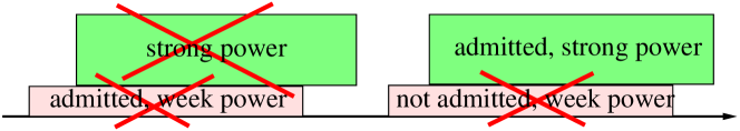
Figure 1: Gain due to admission policy.

A cluster-head needs to synchronize to a packet sent by a sensor before receiving it. In order to synchronize to a packet, the cluster-head has to receive it with some minimum reception power . If the packet reception power is higher than this, cluster-head starts receiving and it continues receiving until the end of the transmission. If the transmission is lost because of the collision with another packet emission (interference), the error will be detected only at the end of the reception. Moreover, this interfering packet will be lost as well since the cluster head was not idle at its arrival epoch; cf. Figure 1.

In order to improve the efficiency, we introduce a packet admission policy. Once the cluster-head is synchronized to a packet, it may decide to receive or ignore the detected packet according to some packet admission policy based, for example, on the value of the received power. This policy allows to ignore some weak packets so that the cluster-head is more often available for stronger packets. The choice of a particular policy depends on system design goals, described in Section II-E.

II-D Sensor placement

Sensors in a given network realization are fixed. We show how to evaluate the performance of a given fixed configuration of sensors served by one cluster head applying some admission policy. For performance optimization, we adopt a stochastic approach. Namely, we optimize the system parameters with respect to the average performance, taken over all possible spatio-temporal configurations of packet emissions, which are driven by some spatio-temporal Poisson point process. We call this model a Poisson-rain process of events. We argue in Appendix A-B1 that this model — which corresponds to the situation where each event is associated with one sensor that activates only once, when the event occurs, and leaves the system afterward — is a reasonable approximation of the packet traffic generated be an arbitrary (also deterministic) repartition of sensors on the plane, provided the density is large. However, it is important to keep in mind that this model is just an approximation, that in reality the sensors are persistent, and that we can collect and keep some information about each one.

II-E Design goals and performance metrics

We consider several design goals, related to the transport of the information from sensors to cluster-heads. Our principal performance metric is the spatio-temporal density $\rho(x)$ of the received information. We define it as the mean number of packets received from sensors, per second, from the surface area $\text{\rm d}x$.

In order to obtain some desired density $\rho(\cdot)$ the system designer can influence the placement of nodes (at least the density), transmission power, and frequency of transmissions. However, while the density of nodes can depend on the location, the transmission power and frequency is the same for all the sensors as we suppose we cannot reconfigure each sensor separately once it is placed. The main parameter that can be tuned in order to shape the information transport from sensors to the cluster-heads is the packet admission policy applied by cluster heads.

In general, the network designer may be interested in maximizing the coverage of some sensing domain or in increasing the total throughput. These contradictory goals are realized by the policies respectively called max-min and globally optimal, which are defined in Sections III-B and III-C;

Finally, the goal of this paper is to propose a hybrid network that will minimize the cost of the network deployment. We thus want to show how much money can a designer save by combining wireless tranceiver sensors with the cheap transmit-only ones. To that respect we study the economic optimization problem in Section III-D, which finds the right proportion of the two types of devices that minimizes the cost of a network, under the constraint of some desired level transport-aware effective coverage.

III Analysis

In this section we will analyze and optimize the performance of the sensors-to-cluster-heads information transport in transmit only sensor network, whose system assumptions are described in Section II. We assume that the density of sensors $\lambda_{s}$ is large enough and the sensing regions are small so as to guarantee a good sensing-coverage of the domain with a sufficient resolution.

III-A Density of information

First, we study the density of information received by a single cluster head $\rho(x)$. Remind that we define it as as the mean number of packets received by the cluster-head per unit of time from the area $\text{\rm d}x$. We will model the traffic described in Section II-A by a spatio-temporal Poisson point process of events (packet transmissions) with intensity $\Lambda_{s}(\text{\rm d}x)\times\lambda_{e}\text{\rm d}t$, where $\Lambda_{s}(\text{\rm d}x)=\lambda_{s}(x)\text{\rm d}x$ and $\lambda_{e}$ are, respectively, the mean number of sensors placed at $\text{\rm d}x$, and the temporal intensity of packet traffic sent by each sensor. This Poisson rain of events (packets) is supposed to be received by one cluster-head, whose behavior is described in Sections II-B–II-C. Specifically, the cluster head applies some admission policy $d(x)$, which is the probability that it tries, given it is idle, to receive a given packet emitted from $\text{\rm d}x$ . We assume that the admission decisions are taken independently of each other and of anything else, and thus the spatio-temporal process of admissible packets is the Poisson process with intensity $d(x)\lambda_{s}(x)\text{\rm d}x\times\lambda_{e}\text{\rm d}t$.

Inspired be the channel description of Section II-B, we assume that a given admissible packet, arriving when the cluster-head is idle, is correctly received if some SINR, empirically averaged over the reception period $B$, is higher than some threshold $\gamma$; cf. (2.1). The interference is created by all other emissions taking place at this time period and by some external noise $W$. A detailed mathematical analysis of the performance of the cluster-head modeled by some Erlang’s loss system with interference and SINR condition (A.1) is done in Section A-B under the assumption of Rayleigh fading. In what follows we summarize the results of this analysis. First, we remind a general fact that follows from the Campbell formula.

Proposition III.1

The density of received information is equal to $\rho(x)=\lambda_{e}\lambda_{s}(x)d(x)p_{free}\,p_{rec}(x)$, where $p_{free}$ is the probability that a typical admissible packet finds the cluster head idle when it arrives and $p_{rec}(x)$ is the conditional probability that the typical admissible packet arriving from $\text{\rm d}x$ can be correctly received, given the cluster head stars receiving it.

Suppose that the cluster-head is located at the origin. Denote by $\bar{P}$ is the emission power used be all sensors, by $L(x)$ the power attenuation function (path-loss) of the distance from $x$ to 0, and by $\mathcal{L}_{W}$ the Laplace transform of the power $W$ of the external (white) noise; $\mathcal{L}_{W}(\xi)=e^{-\xi W}$ if this power is constant.

For a given admissible packet received by the cluster-head, let $\mathcal{L}_{1},\mathcal{L}_{2},\mathcal{L}_{J_{B}}$ be the Laplace transforms of the interference averaged over the reception period, generated respectively, by: admissible packets arriving when it is being received, admissible packets that are being sent at its arrival epoch, all non-admissible packets; cf. Figure 2. These Laplace transforms are explicitly given by formulas (A.11), (A.12), (A.13) with $\lambda=\lambda_{e}\int d(r)\,\lambda_{s}(x)\text{\,\rm d}x$ begin the total intensity of the admissible packets (the integral is taken over the whole domain of the network deployment). Denote $\gamma_{x}=\gamma/(\bar{P}L(x))$. By Corollary A.6, we have the following result.

Proposition III.2

The Erlang acceptance probability is equal to $p_{free}=1/(1+\lambda B)$ and the conditional reception probability is equal to $p_{rec}(x)=\mathcal{L}_{W}(\gamma_{x})\mathcal{L}_{1}(\gamma_{x})\mathcal{L}_{2}(\gamma_{x})\mathcal{L}_{J_{B}}(\gamma_{x})$.

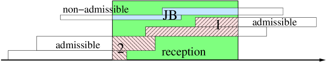
Figure 2: Three terms of interference $\mathcal{L}_{1},\mathcal{L}_{2},\mathcal{L}_{J_{B}}$.

Lets denote

$$\mathcal{L}(\xi)=\exp\biggl{(}\!\!\!-\lambda_{e}B\!\!\!\int\!\!\Bigl{(}1-\frac{1}{\xi\bar{P}L(x)}\log(1+\xi\bar{P}L(x))\,\Lambda_{s}(\text{\rm d}x)\Bigr{)}\!\!\biggr{)}\,.$$ (3.1)

Corollary A.7 gives two more explicit bounds on $p_{rec}(x)$.

Proposition III.3

We have $\underline{p}_{rec}(x)\!\leq\!p_{rec}(x)\!\leq\!\overline{p}_{rec}(x)$, where $\underline{p}_{rec}(x)=\mathcal{L}_{W}(\gamma_{x})\mathcal{L}^{2}(\gamma_{x})$, $\overline{p}_{rec}(x)=\mathcal{L}_{W}(\gamma_{x})\mathcal{L}(\gamma_{x})$ and $\mathcal{L}$ is given by (3.1).

Denote by $\underline{\rho}(x),\overline{\rho}(x)$, respectively, the lower and the upper bound of $\rho(x)$ obtained when $p_{rec}(x)$ in Proposition III.1 is replaced by, respectively, $\overline{p}_{rec}(x)$ and $\underline{p}_{rec}(x)$. Note that the both $\overline{p}_{rec}(x)$ and $\underline{p}_{rec}(x)$ do not depend on $d(\cdot)$ which makes the analysis of $\underline{\rho}(x),\overline{\rho}(x)$ easier (for the quality of the bounds see Figure 5, (left)).

Before describing some optimal policies, we define a naive policy $d_{naive}(x)=\mathbf{1}(x\in{\mathbb{D}}_{0})$, where the set ${\mathbb{D}}_{0}$ is fixed such that mean received power is large enough to receive correctly the packet, given only external noise $W$ (no interference) ; i.e., ${\mathbb{D}}_{0}=\{x:\bar{P}L(x)/W\geq\gamma\}$.

III-B Optimizing the transport-aware coverage

Knowing that the attenuation function $L(x)$ (and thus $p_{rec}(x)$) typically decreases with the distance $|x|$ to the cluster-head, one has to compensate it with an increasing density of sensors $\lambda_{s}(\cdot)$ and/or a spatial admission policy $d(x)$.

In this paper we suppose now that the sensors are already deployed   with some given with density $\lambda_{s}(x)>0$ on some sensing domain ${\mathbb{D}}$. We look for an admission policy $d(x)$, such that any increase of the ratio $\rho(x)/D(x)$ on some set $\text{\rm d}x$ of positive Lebesgue’s measure would be at the expense of decreasing of some already smaller ratio $\rho(y)/D(y)$ on some non-null set $\text{\rm d}y\in{\mathbb{D}}$. The policy ${d_{maxm}}(x,D)$ realizing the above principle is called weighted max-min fair policy, with weights $1/D(x)$. It is known that if ${d_{maxm}}(\cdot,D)$ exists then it is unique. For brevity we will denote by ${d_{maxm}}(x)$ the max-min policy with equal weights ($D(x)=D$) (the policy does not depend on the value of $D$).

We cannot exactly characterize the max-min fair policy for $\rho(x)$, however, we can do this for some bounds. Denote $\underline{I}=\int_{{\mathbb{D}}}D(x)/\underline{p}_{rec}(x)\text{\,\rm d}x$. Assume that the sensing domain ${\mathbb{D}}$ is compact, $D(x)$ continuous on ${\mathbb{D}}$ and denote $\underline{M}=\max_{x\in{\mathbb{D}}}D(x)/(\lambda_{s}(x)\overline{p}_{rec}(x))$. We define in the similar manner $\overline{I},\overline{M}$ replacing $\underline{p}_{rec}(x)$ in the above formulas by $\overline{p}_{rec}(x)$.

For a given policy $d(\cdot)$ denote by $||d||_{\lambda_{s}}=\int_{{\mathbb{D}}}d(x)\lambda_{s}(x)\text{\,\rm d}x$ the total spatial intensity of admissible packets under $d(\cdot)$.

Proposition III.4

• The max-min fair policy $\underline{d}_{maxm}(\cdot,D)$ for $\underline{\rho}(x)$ on ${\mathbb{D}}$ exists if and only if $\underline{M}<\infty$, it is equal to

  $$\underline{d}_{maxm}(x,D)=\frac{D(x)}{\underline{M}\lambda_{s}(x)\underline{p}_{rec}(x)}\,$$ (3.2)

  and realizes $\underline{\rho}_{maxm}(x,D)=D(x)/(B\underline{I}+\underline{M}/\lambda_{e})$. Moreover, under $\underline{d}_{maxm}(\cdot,D)$ we have $\rho(x)\geq\underline{\rho}_{maxm}(x,D)$.

• The max-min fair policy $\overline{d}_{maxm}(\cdot,D)$ for $\overline{\rho}(x)/D(x)$ on ${\mathbb{D}}$ exist if and only if $\overline{M}<\infty$, it is given by (3.2) with $\underline{M},\underline{p}_{rec}$ replaced, respectively, by $\overline{M},\overline{p}_{rec}$, and realizes $\overline{\rho}_{maxm}(x,D)=D(x)/(B\overline{I}+\overline{M}/\lambda_{e})$. Moreover, there is no policy $d(\cdot)$ for which $\rho(x)\geq\overline{\rho}_{maxm}(x,D)$, with the strict inequality on some non-null set $\text{\rm d}x$.

Proof:

We consider the lower bound. The proof for the upper bound is analogous. Suppose that $\underline{M}<\infty$. Note that the function given by the right-hand-side of (3.2) in positive and not larger than 1. Thus $\underline{d}_{maxm}(\cdot,D)$ is a policy. Note also that for $x_{0}=\mathop{\text{\rm arg~{}max}}_{x\in{\mathbb{D}}}D(x)/(\lambda_{s}(x)\underline{p}_{rec}(x))$ we have $\underline{d}_{maxm}(x_{0},D)=1$. Assume now that for some policy $d^{\prime}(x)$ the respective ratio $\underline{\rho}^{\prime}(x)\geq D(x)1/(B\underline{I}+M/\lambda_{e})$ and that the inequality is strict on some non-null set $\text{\rm d}x$. It easy to show that then $||d^{\prime}||_{\lambda_{s}}>||\underline{d}_{maxm}||_{\lambda_{s}}$ and thus $\underline{\rho}^{\prime}(x_{0})<\underline{\rho}(x_{0})$. This shows that $\underline{d}_{maxm}$ is max-min fair.

Suppose now that $M=\infty$. Take any policy $d(\cdot)$. Note that $\underline{\rho}(x)/D(x)$ cannot be constant under this policy (there is no such policy). Thus, there exist $x_{1},x_{2}$ such that $\underline{\rho}(x_{1})>\underline{\rho}(x_{2})$. Note that we can slightly increase $d(x_{1})$ and decrease $d(x_{2})$ is such a manner that $||d||_{\lambda_{s}}$ remains constant. This increases $\underline{\rho}(x_{2})$ without changing $\underline{\rho}(x)$ for $x\not=x_{1},x_{2}$. Thus, $d(\cdot)$ is not a max-min fair. The remaining part of the result follows from Proposition III.3. ∎

Remark: Suppose the cluster-head is to collect information sent by sensors in a given compact domain ${\mathbb{D}}$ with some minimal density $\rho(x)\geq D(x)$. The problem might be infeasible. However, if it is, policy ${d_{maxm}}(x,D)$ satisfies the constraint.

Example III.5

Consider a uniform coverage $D(x)=D\times\mathbf{1}(x\in{\mathbb{D}})$ witght function. We might be interested in maximizing the constant density $D$ given the domain ${\mathbb{D}}$. This is achieved using ${d_{maxm}}$. Alternatively, we might be interested in maximizing the area of domain ${\mathbb{D}}$ while providing some minimal density $D$. For example, for a homogeneous repartition of sensor $\lambda_{s}(x)=\lambda_{s}$ and distance-dependent path-loss $L(x)=L(|x|)$ model, we maximize the radius $R$ of the disk ${\mathbb{D}}=B(0,R)$ centered at 0, under the contranit $\rho(x)\geq D$ for $x\in{\mathbb{D}}$. Using Proposition III.4 one can find the solution $R=\underline{R}_{maxm}$ such that policy $\underline{d}_{maxm}$ on ${\mathbb{D}}=B(0,\underline{R}_{maxm})$ satisfies $\rho(x)\geq\underline{\rho}(x)=D$ for all $x\in{\mathbb{D}}$. We illustrate this problem in Section IV.

III-C Optimizing the total throughput

Consider now the problem of the maximization of the total weighted intensity of received information $U=\int_{{\mathbb{D}}}\rho(x)/D(x)\text{\,\rm d}x\,,$ where $D(x)>0$ are some arbitrary weights.

Denote by $\underline{U},\overline{U}$, respectively, the lower and the upper bound of the total weighted intensity of information obtained when $\rho(x)$ is replaced by $\underline{\rho}(x)$ and $\overline{\rho}(x)$. As previously, we can solve this global optimization problem for the bounds $\underline{\rho}(x)$ and $\overline{\rho}(x)$, and in this way approximate the solution of the original problem.

Denote the following water-filling region $\underline{{\mathbb{D}}}(\theta)=\{x\in{\mathbb{D}}:\lambda_{s}(x)\underline{p}_{rec}(x)/D(x)>\theta\}$ and the constant

$$\underline{\theta}^{*}=\mathop{\text{\rm arg~{}max}}_{\theta}\frac{\int_{\underline{{\mathbb{D}}}(\theta)}\lambda_{s}(x)\underline{p}_{rec}(x)/D(x)\text{\,\rm d}x}{1+\lambda_{e}B\int_{\underline{{\mathbb{D}}}(\theta)}\lambda_{s}(x)\text{\,\rm d}x}\,.$$

We define in the similar manner $\overline{\mathbb{D}},\overline{\theta}^{*}$ replacing $\underline{p}_{rec}(x)$ in the above formulas by $\overline{p}_{rec}(x)$.

Proposition III.6

• The policy $\underline{d}^{*}(x)=\mathbf{1}(x\in\underline{{\mathbb{D}}}(\underline{\theta}^{*})$ maximizes $\underline{U}$. Under this policy

  $$\underline{U}=\underline{U}^{*}=\frac{\lambda_{e}\int_{\underline{{\mathbb{D}}}(\underline{\theta}^{*})}\lambda_{s}(x)\underline{p}_{rec}(x)/D(x)\text{\,\rm d}x}{1+\lambda_{e}B\int_{\underline{{\mathbb{D}}}(\underline{\theta}^{*})}\lambda_{s}(x)\text{\,\rm d}x}\,.$$ (3.3)

  Moreover, under $\underline{d}^{*}(\cdot)$ we have $U\geq\underline{U}^{*}$.

• The policy $\overline{d}^{*}(x)=\mathbf{1}(x\in\overline{\mathbb{D}}(\overline{\theta}^{*})$ maximizes $\underline{U}$. Under this policy $\overline{U}=\overline{U}^{*}$ it is given by (3.3) with $\underline{{\mathbb{D}}},\underline{\theta}^{*}$ replaced, respectively, by $\overline{\mathbb{D}},\overline{\theta}^{*}$, Moreover, there is no policy $\d{(}\cdot)$ under which $U>\overline{U}^{*}$.

Proof:

We consider the lower bound problem (proof for the upper bound is analogous): maximize $\int_{\mathbb{D}}\lambda_{s}d(x)\underline{p}_{rec}(x)/D(x)\text{\,\rm d}x/(1-\lambda_{e}BA)$ under the constraints: $A=\int_{{\mathbb{D}}}\lambda_{s}(x)d(x)\text{\,\rm d}x$, $0\leq d(x)\leq 0$. We write the Lagrangian

$$L(d,\theta,\mu_{0},\mu_{1})=\theta A+\int_{{\mathbb{D}}}\mu_{1}(x)\text{\,\rm d}x$$

$$+\int_{{\mathbb{D}}}d(x)\Bigl{(}\frac{\lambda_{s}(x)\underline{p}_{rec}(x)/D(x)}{1+\lambda_{e}BA}-\theta+\mu_{0}(x)-\mu_{1}(x)\Bigr{)}\text{\,\rm d}x\,.$$

By the strong duality and the KKT conditions the optimal policy has the form of the indicator function $\underline{d}^{*}(x)=\mathbf{1}\bigl{(}\lambda_{s}(x)\underline{p}_{rec}(x)/(D(x)(1+\lambda_{e}BA^{*}))\leq\theta^{*}\bigr{)}$ for some $\theta^{*},A^{*}$. The values of these constants are found by the standard watter-filling policy. The remaining part of the result follows from Proposition III.3. ∎

Example III.7

Consider equal weights $D(x)=D$, homogeneous repartition of sensors and and distance-dependent path-loss model. Then ${\mathbb{D}}(\underline{\theta}^{*})=B(0,\underline{R}^{*})$ is a dics of radius $\underline{R}^{*}$  We illustrate this finding numerically in Section IV.

III-D Optimizing the network cost

Suppose that one transmit-only sensor costs $C_{s}$, while a transport-reliable sensor (with the same sensing functionality) costs $C_{c}$. Consider an architecture where the transport-reliable sensors act as cluster-heads considered previously in this paper; call them cluster-heads. Assume that information obtained (sensed) directly by cluster-heads sensors is delivered to the central unit with probability one, while the information obtained by a transmit-only sensor located at $x$ is delivered there with probability $p_{rec}(x-Z^{*}(x))$ where $Z^{*}$ is the location of the cluster-head nearest to $x$.

In order to formalize the problem of the economic optimization of the proportion of the two types of devices, let us assume a regular repartition of cluster heads on the plane. A simple model consists in taking them to be repartitioned on a regular, say, triangular grid with some density $\lambda_{c}$. This means that $\lambda_{c}=4/(L^{2}\sqrt{3})$, where $L$ is the distance between two adjacent cluster-heads. Note that maximal distance to a nearest cluster head is equal to $R_{\max}(\lambda_{c})=4/\sqrt{\lambda_{c}3\sqrt{3}}$. As as in the previous section we model the traffic of packets sent be the sensors to the cluster-heads (who act independently) by Poisson rain model of events that is assumed to be stationary both in time and on the whole plane ${\mathbb{R}}^{2}$. To further simplify the model, we assume that at each point $x$ in space at least one cluster-head has to achieve $\rho(x)\geq D$. This is an upper bound on $\lambda_{c}$; in reality, a packete that is lost by a cluster-head, may still be captured by another cluster-head. However, this upper-bound is sufficient to numerically demonstrate large savings of the hybrid approach.

Consider the following problem: minimize the cost of the network by unit area $C=\lambda_{s}C_{s}+\lambda_{c}C_{c}$ given some minimal intensity of received information $\lambda_{e}\lambda_{c}+\rho(R_{\max})\geq D$, where $\lambda_{e}\lambda_{c}$ is the density of information captured directly by the cluster-heads and $\rho(R_{\max})$ is the lowest density of information that can by obtained from the sensors given max-min (maximizing coverage) admission policy.

In order to solve this problem, given $D$ and $\lambda_{e},\lambda_{s}$, we take the max-min policy $\underline{d}_{maxm}$ (3.2) with $D(x)=\mathbf{1}(|x|\leq R)$ and find the maximal radius $\underline{R}_{maxm}$, such that the constant $\underline{\rho}_{maxm}$ obtained by the policy $D(x)=\mathbf{1}(|x|\leq\underline{R}_{maxm})$ on $B(0,\underline{R}_{maxm})$ is equal to $D-\lambda_{e}\lambda_{c}$ (cf. Example III.5). Note by Proposition III.4 that for all $x$, $\rho(x)\geq\underline{\rho}(x)\geq\underline{\rho}_{maxm}(\underline{R}_{maxm})=D-\lambda_{e}\lambda_{c}$. This means that taking $R_{\max}=\underline{R}_{maxm}$; i.e., $\lambda_{c}=4/(\underline{R}_{maxm}^{2}3\sqrt{3})$ is sufficient for $\lambda_{e}\lambda_{c}+\rho(R_{\max}(\lambda_{c}))\geq D$. Having calculated $\lambda_{c}=\lambda_{c}(\lambda_{s})$ we express the cost of the network $C=C(\lambda_{c}/\lambda_{s})$ as the function the proportion between the intensity of cluster-heads and the sensors. Finally, we look for its maximal value.

IV Numerical results

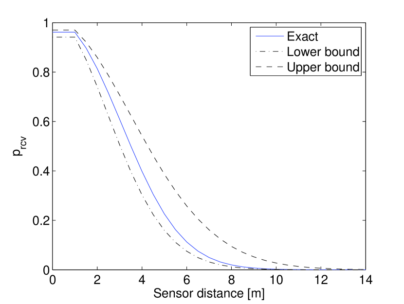
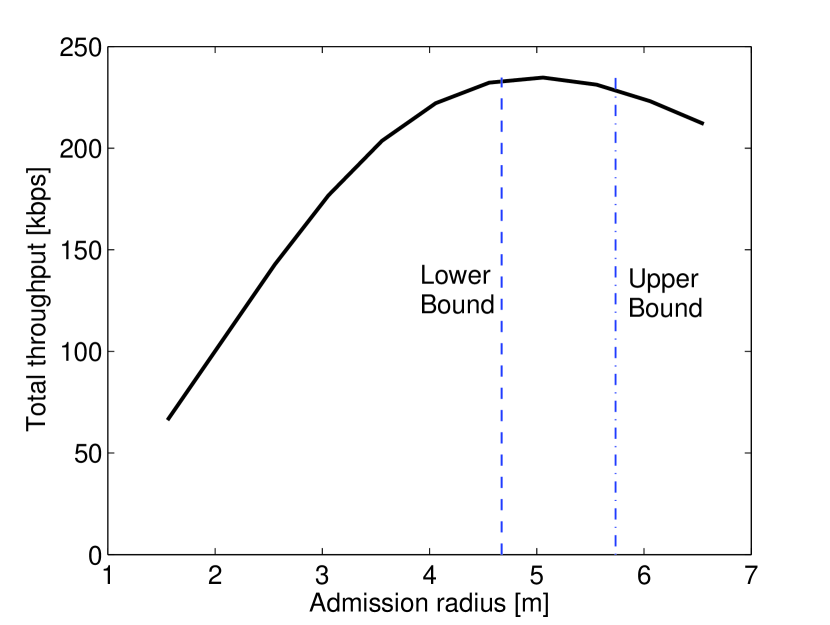
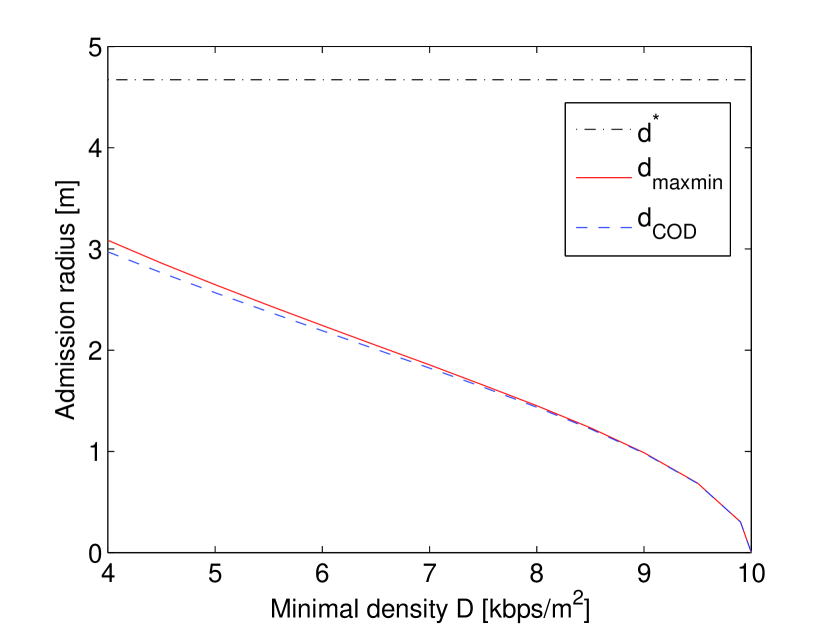
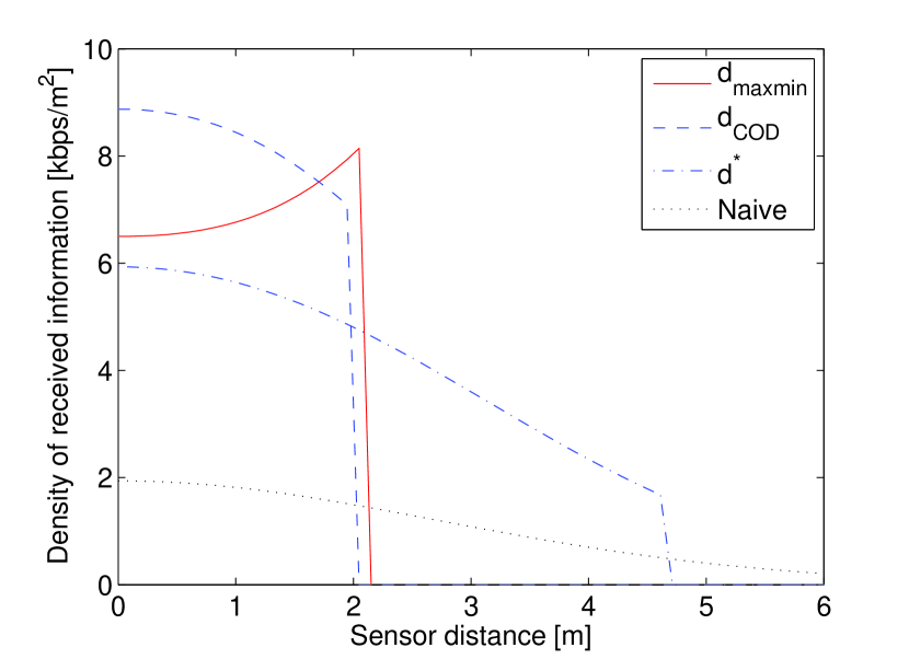
Figure 3: Exact value and approximations of $p_{rec}$ (left). Maximization of the total intensity of information (right).

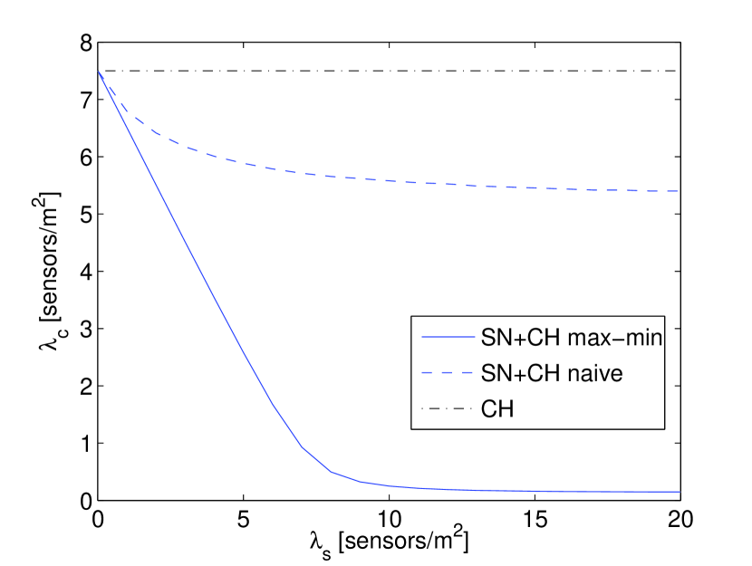
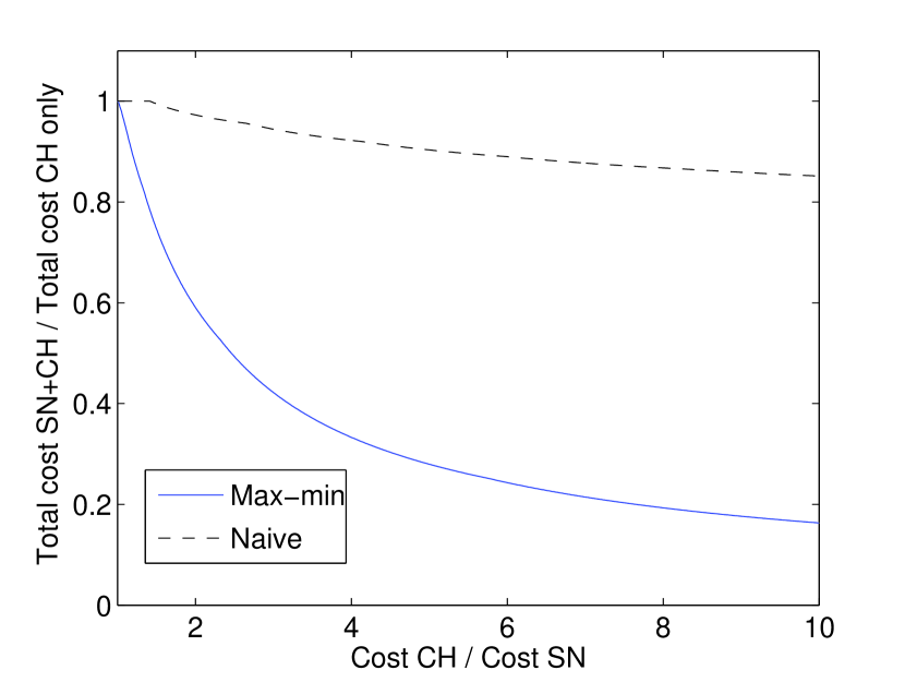
Figure 4: Radii of different admission policies (left). The exact profiles of $\rho(x)$ for different admission policies (right) when applying different admission policies explicitly found using the lower-bound $\underline{\rho}$ (this explains why the max-min policy does not give exactly $\rho(x)=const$ for $x$ within the admission distance).

Figure 5: Constitution of the hybrid network (cluster-heads CH and transmit-only sensors SN) with minimal cost, assuring $\min_{x}\rho(x)=0.75$ (right). Network cost gain in function of the device cost per unit ratio (right).

We will give now some numerical examples. We consider the canonical traffic scenario described in Section II-A with SINR threshold $\gamma=1$, path-loss model $L(x)=L(|x|)=\kappa|x|^{-\eta}$ with $\kappa=10^{-5.5}$, $\eta=3.3$.

Single cluster-head scenario

In this part we consider a scenario with a single cluster-head at 0. Figure 5 (left) shows the the quality of approximations given in Proposition III.3.

Next we compare maximum radii of different admission policies. In addition to $\underline{d}_{maxm}$ and $\underline{d}^{*}$, defined in Section III-B and Section III-C respectively, we introduce the coverage-optimal deterministic (COD) policy. It is defined as $d_{COD}(x)=\mathbf{1}(|x|\leq R_{COD})$ where $R_{COD}$ is the maximum radius such that $\rho(R_{COD})\geq D$ under policy $d_{COD}$.

We can see from the results in Figure 5 (left) that $\overline{R}_{maxm}\approx R_{COD}$, hence that a deterministic policy with a well-chosen radius provides almost as good coverage as the max-min fair policy. In addition, we see from Figure 5 (right) that COD policy is more efficient. A more detailed discussion on a tradeoff between efficiency and fairness is out of the scope.

Figure 5 (right) shows the total intensity $U$ of information obtained when the admission policy accepts all the packet within a given radius. Optimal policy radius (maximizing the total throughput) can be deduced from this plot. Two marked radii correspond to policies $\underline{d}^{*},\overline{d}^{*}$.We see that the policies $\underline{d}^{*},\overline{d}^{*}$ well approximate the optimal. We also see on Figure 5 (right) that maximizing capacity requires admission region $\underline{R}^{*}$ that is much larger than $\underline{R}_{maxm}$ and $R_{COD}$, having significantly smaller $\rho(x)<\underline{\rho}_{maxm}(x)$.

Economic optimization

We now look at the economic aspects, described in Section III-D. Figure 5 (left) shows the required density of cluster-heads in the hybrid network in function of the density of transmit-only sensors, given the minimal value $\min_{x}\rho(x)=\rho(R_{\max})=0.75$. Figure 5 (right) shows the network cost economization in function of the cluster-head/sensor unit cost ratio. We can see that even when a price of a cluster-head is only slightly higher than a price of a transmit-only sensor, we can achive significant savings. On a contrary, using the naive policy, cost savings are negligable.

V Implementation issues and concluding remarks

In this paper, we analyzed hybrid sensor networks consiting of transceiving and transmit-only sensors. We presented a detailed mathematical model of a physical and MAC layer of the network. Using this model we derived the optimal packet admission policies for cluster-head that maximize coverage or total throughput. Also, using the model we demonstrated how much the dollar-cost of a sensor network can be decreased while maintaining the same network coverage. The MAC model that we developed can also be used for any non-slotted wireless communication channel.

In this work we did not discuss implementation details of the optimal policies. However, we note that these policies can easily be implemented, based only on the knowledge of packet received power (no need to know channel attenuation function, sensor positions, etc). One implementation is discussed in [1], and can easily be generalized to the policies proposed in this paper. We leave details for future work.

Also, in this work we optimized only packet admission policy and not the sensor density $\lambda_{s}(x)$, transmitting power $\overline{P}(x)$, coding $\gamma(x)$ nor the transmission frequency $\lambda_{e}(x)$, which may depend on particular sensors. However, we showed that even constrainted on the optimization of the admission policy only, we can achieve large savings and maintaint architecture simple. Optimizing other parameters is left for the future work.

Appendix: Mathematical modeling

In this section we present mathematical models that are used to analyze the sensor network described in Section II. In particular,

A-A An Erlang’s M/D/1/1 loss system with interference

Assume a time homogeneous, independently marked Poisson point process $\Phi=\{(T_{n},(P_{n},H_{n}))\}_{n=-\infty}^{\infty}$, where $T_{n}$ are customer (packet) arrival epochs and $(P_{n},H_{n})$ are independent, identically distributed (i.i.d.) marks, where $P_{n}\geq 0$, $H_{n}\geq 0$ can be interpreted as, respectively, the average (over fading effects) power with which the $n\,$th packet arrives at the receiver and the actual fading state of its channel. (The randomness of $\{P_{n}\}$ reflects different locations of transmitters and powers with which they emit packets, while the randomness of $\{H_{n}\}$ reflects the temporal variation of the channel conditions given fixed location of the transmitter and emitted power.) Lets denote by $\lambda$ ($0<\lambda<\infty$) the intensity of $\Phi$; i.e., $T_{n}$ are i.i.d. exponential r.v. with parameter $\lambda$.

We consider the following modification of the Erlang’s loss policy. Suppose that each arrival (i.e., packet) is admitted by the single server of the system (i.e., starts being received by the receiver) if this latter is idle at the packet’s arrival epoch and rejected otherwise. Admitted packets are received during their duration time $B$. However, packets that are rejected by the receiver interfere during their emission time with the packets that are being received. Inspired by inequality (2.1), with $H_{n}P_{n}=|h|^{2}P_{rec}$, we will say that the $n\,$th packet, given it is admitted by the receiver, is correctly received if the following inequality holds

$$\frac{P_{n}H_{n}}{W+1/B\int_{T_{n}}^{T_{n}+B}I(t)\text{\,\rm d}t-P_{n}H_{n}}\geq\gamma\,,$$ (A.1)

where $W$ is some nonnegative r.v. independent of $\Phi$, $\gamma>0$ is some constant, $I(t)$ is the value of the following temporal shot-nose process at time $t$

$$I(t)=\sum_{i=-\infty}^{\infty}H_{i}P_{i}\mathbf{1}_{[0,B)}(t-T_{i})\,$$ (A.2)

describing the total power received at time $t$ from all packets that are being sent (including the power of the packet that is being received; this is why we substract $P_{n}H_{n}$ from $I(t)$ in (A.1).

Our goal is to calculate the frequency of the correct reception of packets; i.e., $\pi=\lim_{N\to\infty}\#\{\text{packets received among packets nr.\ }1,\ldots,N\}/N$, where $\#$ denotes the number. Denote by $X(t)$ the indicator of the event that the receiver is busy at time $t$ and $X(-0)=\lim_{t\uparrow 0}X(t)$. Denote by $\delta_{n}$ the indicator of the event that the inequality (A.1) holds. Let $\mathbf{P}^{0}$ denote the Palm probability given there is a customer arrival at time $0$, and let ${\mathbf{E}}^{0}$ denote the corresponding expectation. By Slivnyak’s theorem, under $\mathbf{P}^{0}$ arrivals form the original stationary Poisson point process with an extra arrival $(T_{0},(P_{0},H_{0}))$ added at time $T_{0}=0$ whose mark is independent and originally distributed. Denote by $\mathbf{P},{\mathbf{E}}$, respectively, the stationary probability of $\Phi$ and its corresponding expectation. The following results is a consequence of the ergodic theorem (see e.g. [11, Theorem 1.6.1]).

Proposition A.1

The limit defining $\pi$ exists $\mathbf{P}^{0}$ almost surely and $\pi={\mathbf{E}}^{0}[(1-X(-0))\delta_{0}]$.

In order to calculate $\pi$ we will first characterize under $\mathbf{P}^{0}$ the distribution of the shot noise process $I^{\prime}(t)=I(t)-P_{0}H_{0}$ for $t\in[0,B)$ given the server is idle just before time 0 (i.e., $X(-0)=0$). It will be given in terms of the conditional joint Laplace transform $\mathcal{L}^{0}_{I^{\prime}(t_{1}),\ldots,I^{\prime}(t_{n})|X(-0)=0}(\xi_{1},\ldots,\xi_{n})={\mathbf{E}}^{0}\bigl{[}e^{-\sum_{i=1}^{n}I^{\prime}(t_{i})\xi_{i}}\big{|}X(-0)=0\bigr{]}$ evaluated for $\xi_{i}\geq 0$ and any finite collection of time instants $t_{1},\ldots,t_{n}\in[0,B)$, $n\geq 1$.

Proposition A.2

Consider the Erlang’s M/D/1/1 loss system with interference. Then

$$\mathbf{P}^{0}\{X(-0)=0\}=\frac{1}{1+\lambda B}$$ (A.3)

and for $t_{1},\ldots,t_{n}\in[0,B)$, $n\geq 1$, $\xi_{1},\ldots,\xi_{n}\geq 0$

$$\mathcal{L}^{0}_{I^{\prime}(t_{1}),\ldots,I^{\prime}(t_{n})|X(-0)=0}(\xi_{1},\ldots,\xi_{n})$$

$$= \int_{0}^{\infty}\lambda e^{-\lambda t}\exp\Bigl{[}-\lambda\int_{-B}^{B}\Bigl{(}1-\mathbf{1}_{(-t,0]}(s)\Bigr{)}$$

$$\times\Bigl{(}1-{\mathbf{E}}[e^{-\sum_{i=1}^{n}\xi_{i}H_{i}P_{i}\mathbf{1}_{[0,B)}(t_{i}-s)}\Bigr{)}\text{\,\rm d}s\Bigr{]}\text{\,\rm d}t\;.$$

Note by the form of the above Laplace transform, that under $\mathbf{P}^{0}$ and given the server is idle just before the arrival of the customer at $0$, the shot-noise process of interference $\{I^{\prime}(t):0\leq t<B\}$ is driven by a non-homogeneous, double-stochastic Poisson process with intensity equal to $\lambda$ on the sum of the intervals $(-B,-T]\cup(0,B)$ and 0 elsewhere, where $T$ is exponential random variable with parameter $\lambda$.

Proof:

Note that (A.3) follows directly from the Erlang’s loss formula (see e.g. [12, equation (81), p. 71]). In consequence, $\lambda/(1+\lambda B)$ is the intensity of the point process of arrivals of packets that are accepted by the receiver. In order to prove the remaining part of the proposition, lets define by $T(t)$ the time that elapsed form the last moment before $t$ when the receiver was busy; i.e., $T(t)=t-\sup\{s:s<t,X(s)=1\}$. We will first show that under $\mathbf{P}^{0}$ and given $X(-0)=0$, the variable $T=T(0)$ is exponential with parameter $\lambda$. Indeed, for $u>0$, by the Neveu exchange formula (see e.g. [11, Section 1.3.2]),

$$\mathbf{P}^{0}\{\,T(0)\geq u,X(-0)=0\,\} = \mathbf{P}^{0}\{\,T(0)\geq u\,\}$$ (A.5)

$$=\frac{1}{1+\lambda B}\,{\mathbf{E}}^{0}_{a}\biggl{[}\int_{(0,T_{1}^{a}]}\mathbf{1}(T(t)\geq u)\,\Phi(\text{\rm d}t)\biggr{]}\,,$$

where ${\mathbf{E}}^{0}_{a}$ corresponds to the Palm probability, given a packet arriving at time 0 is accepted by the receiver, $T_{1}^{a}$ is the next arrival time after 0 of a packet accepted by the receiver, and the integral with respect to $\Phi(\text{\rm d}t)$ denotes the sum over all arrival times of the process $\Phi$. It is easy to see that under ${\mathbf{E}}^{0}_{a}$ we have $T(t)=0$ for $t\in(0,B]$ and $T(t)=t-B$ for $t\in(B,T_{1}^{a}]$. In the interval $(B,T_{1}^{a}]$ point process $\Phi$ has just one point, namely $T_{1}^{a}$, and thus the integral in (A.5) reduces to $\mathbf{1}(T(T_{1}^{a})\geq u)=\mathbf{1}(T_{1}^{a}-B\geq u)$. The distribution of the points of $\Phi$ in $(0,\infty)$ is not influenced by the condition that the server is idle just before $0$ and that there was an arrival at $0$. Thus, under ${\mathbf{E}}_{a}^{0}$, as well as under ${\mathbf{E}}$, it is equal to the distribution of points of the the original Poisson point process. Thus, due to the lack of memory of the exponential inter-arrival r.v., the variable $T_{1}^{a}-B$ is exponential with parameter $\lambda$, which completes this part of the proof.

Note now, that the packets which contribute to $I^{\prime}(t)=I(t)-P_{0}H_{0}$ for $t\in[0,B)$, given $T(0)=T$ and $T_{0}=0$, arrive only during the time intervals $(-B,-T)\cup(0,B)$. (Note that $\mathbf{P}^{0}($ there is an arrival at $-T)=0$ if $T>0$.) Note also, that this set is disjoint with the set $\mathcal{S}=[T^{*},-B-T(0)]\cup[-T(0),0]$, where $T^{*}=\sup\{T_{n}:T_{n}<T(0)-B,T_{n+1}<T(0)-B,T_{n+1}-T_{n}>B\}$. This latter set is a random stopping set (i.e., for a given realization $\phi$ of the point process $\Phi$, the set $\mathcal{S}(\phi)$ is invariant with respect to any modification of the points of $\phi$ in ${\mathbb{R}}\setminus\mathcal{S}(\phi)$; see e.g. [13]). Also, $X(-0)$ and $T(0)$ depend only on the configuration of points of $\phi$ in $\mathcal{S}(\phi)$. Thus, by the strong Markov property of the Poisson point process (see [13]), given $X(-0)=0,T=T(0)$, the distribution of arrivals in $(-B,-T)\cup(0,B)$ is equal to the original distribution of points of the independently marked Poisson point process $\Phi$ taken on this region, and hence (A.2) holds. This completes the proof. ∎

Before we give an explicit formula for the frequency $\pi$ of the correct reception of packets for our loss system with interference in the case of Rayleigh fading, we will calculate the conditional Laplace transform of the integrated shot-noise $I^{\prime}_{B}=1/B\int_{0}^{B}I^{\prime}(t)\text{\,\rm d}t$ given $\mathbf{P}^{0}$ and $X(-0)=0$; i.e., $\mathcal{L}^{0}_{I^{\prime}_{B}|X(-0)=0}(\xi)={\mathbf{E}}^{0}\bigl{[}e^{-\xi I^{\prime}_{B}}\big{|}X(-0)=0\bigr{]}$ for $\xi\geq 0$.

Proposition A.3

Suppose $\{H_{n}\}$ are exponentially distributed with mean 1 and $\{P_{n}\}$ are independent of $\{H_{n}\}$. Then $\mathcal{L}^{0}_{I^{\prime}_{B}|X(-0)=0}(\xi)=\mathcal{L}_{1}(\xi)\mathcal{L}_{2}(\xi)$, where

$$\mathcal{L}_{1}(\xi) = \exp\biggl{(}-\lambda B\Bigl{(}1-{\mathbf{E}}\Bigl{[}\frac{1}{\xi P}\log(1+\xi P)\Bigr{]}\Bigr{)}\biggr{)}\,,$$ (A.6)

$$\mathcal{L}_{2}(\xi) = \exp(-\lambda B)$$

$$\times \!\!\!\!\!\biggl{(}1+\lambda B\int_{0}^{1}\exp\biggl{(}\lambda B{\mathbf{E}}\Bigl{[}\frac{1}{\xi P}\log(1+\xi Pt)\Bigr{]}\biggr{)}\text{\,\rm d}t\biggr{)}\,.$$

Proof:

Note first, that the integrated shot noise is also a shot noise type variable. Indeed, $I^{\prime}_{B}=1/B\int_{0}^{B}\sum_{i\not=0}H_{i}P_{i}\mathbf{1}_{[0,B)}(t-T_{i})=\sum_{i\not=0}H_{i}P_{i}V(T_{i})$, where $V(t)$ is equal to $B-|t|$ for $|t|\leq B$ and 0 elsewhere. By the Proposition A.2, it suffices to calculate the Laplace transform of $I^{\prime}_{B}$ driven by independently marked double-stochastic Poisson process with intensity $\lambda$ on the sum of the intervals $(-B,-T]\cup(0,B)$ where $T$ is exponential random variable with parameter $\lambda$. Denote

$$I^{1}_{B} = \sum_{i\not=0}H_{i}P_{i}V(T_{i})\mathbf{1}_{(0,B)}(T_{i})\,,$$ (A.8)

$$I^{2}_{B} = \sum_{i\not=0}H_{i}P_{i}V(T_{i})\mathbf{1}_{(-B,-T]}(T_{i})\,.$$ (A.9)

Applying the general formula of the Laplace transform of the independently marked Poisson point process (see e.g. [14])) we get

$${\mathbf{E}}^{0}[e^{-\xi I^{1}_{B}}|X(-0)=0]=\exp\biggl{(}-\lambda\!\!\!\int_{0}^{B}\!\!\!\Bigl{(}1-{\mathbf{E}}\Bigl{[}e^{-\xi HPV(t)}\Bigr{]}\Bigr{)}\text{\,\rm d}t\biggr{)}\,,$$ (A.10)

where $H,P$ are independent, generic r.v’s for $\{H_{n}\}$ and $\{P_{n}\}$. Integrating with respect to $t$ and evaluating expectation with respect to the exponential r.v. $H$ we obtain ${\mathbf{E}}[e^{-\xi I^{1}_{B}}]=\mathcal{L}_{1}(\xi)$. In order to calculate ${\mathbf{E}}^{0}[e^{-\xi I^{2}_{B}}|X(-0)=0]$, we condition on $T=T(0)$ and we use similar arguments, with integral $\int_{0}^{B}$ in (A.10) replaced be $\int_{-B}^{-T}$ (note that this integral is null if $T>B$). Similarly as for $I^{1}_{B}$ and then by integration with respect to the law of exponential $T$ we obtain ${\mathbf{E}}^{0}[e^{-\xi I^{2}_{B}}|X(-0)=0]=\mathcal{L}_{2}(\xi)$. Obviously $I^{\prime}_{B}=I^{1}_{B}+I^{2}_{B}$, and variables $I^{1}_{B},I^{2}_{B}$ are independent, because they are driven by disjoint regions of the underlying Poisson point process. Thus $\mathcal{L}^{0}_{I^{\prime}_{B}}(\xi)=\mathcal{L}_{1}(\xi)\mathcal{L}_{2}(\xi)$, which completes the proof. ∎

Now we are able to give the main result of this Section — an Erlang’s type formula.

Proposition A.4

Consider the Erlang’s M/D/1/1 loss system with interference. Suppose that $\{H_{n}\}$ are exponential r.v’s independent of $\{P_{n}\}$ and lets denote by $\mathcal{L}_{W}(\xi)$ the Laplace transform of $W$. Then

$$\pi=\frac{1}{1+\lambda B}{\mathbf{E}}\Bigl{[}\mathcal{L}_{W}(\gamma/P_{0})\mathcal{L}_{1}(\gamma/P_{0})\mathcal{L}_{2}(\gamma/P_{0})\Bigr{]}\,,$$

where the expectation is taken with respect to the random variable $P_{0}$.

Proof:

By Proposition A.1 $\pi$ is equal to

$${\mathbf{E}}^{0}[(1-X(-0))\delta_{0}]$$

$$=\mathbf{P}^{0}\{\,X(-0)=0\,\}\,{\mathbf{E}}^{0}[\delta_{0}|X(-0)=0]$$

$$=\mathbf{P}^{0}\{\,X(-0)\,\}\,\mathbf{P}^{0}\Bigl{\{}\,H_{0}\geq\gamma W(W+I^{\prime}_{B})/P_{0}\Big{|}X(-0)=0\,\Bigr{\}}$$

$$=\mathbf{P}^{0}\{\,X(-0)=0\,\}\,{\mathbf{E}}^{0}\Bigl{[}\exp\Bigl{(}-\gamma(W+I^{\prime}_{B})/P_{0}\Bigr{)}\Big{|}X(-0)=0\Bigr{]}$$

because $H_{0}$ is exponential with mean 1 and independent of everything else. Conditioning on $P_{0}$, noting that $W$ is independent of $I^{\prime}_{B}$ and using Propositions A.2 and A.3 we obtain the result. ∎

Lets introduce now to the Erlang’s loss model an additional (external) stationary, ergodic process $J(t)$ of interference, independent of $W$ and $\Phi$. (For example, one can think of $J(t)$ as of the interference created by emitters transmitting packets that are not supposed to be received by our receiver due to some random, independent admission policy; cf. Section A-B). Lets say that the $n\,$th packet of $\Phi$, given it is admitted by the receiver, is correctly received if to the inequality (A.1) holds with the term $1/B\int_{T_{n}}^{T_{n}+B}J(t)\text{\,\rm d}t$ added to the denominator. Denote by $\delta^{\prime}_{n}$ the indicator of this event. and $\pi^{\prime}={\mathbf{E}}^{0}[(1-X(-0))\delta^{\prime}_{0}]$. Denote by $J_{B}=\int_{0}^{B}J(t)\text{\,\rm d}t$ and its Laplace transform by $\mathcal{L}_{J_{B}}(\xi)={\mathbf{E}}[e^{-\xi J_{B}}]$. We have the following straightforward extension of the Proposition A.4.

Corollary A.5

Consider the Erlang’s M/D/1/1 loss system with the external interference $J(t)$. Under the same assumptions as in Proposition A.4 the frequency of the correct reception of packets exists $\mathbf{P}^{0}$ almost surely and is equal to

$$\pi^{\prime}=\frac{{\mathbf{E}}\bigl{[}\mathcal{L}_{W}(\gamma/P_{0})\mathcal{L}_{1}(\gamma/P_{0})\mathcal{L}_{2}(\gamma/P_{0})\mathcal{L}_{J_{B}}(\gamma/P_{0})\bigr{]}}{1+\lambda B}\,.$$

A-B Sensors on the plane

In this section we assume that the packets are emitted from different locations of the plane ${\mathbb{R}}^{2}$ and, assuming some form of the attenuation function, we will obtain a particular form of the distribution of the powers $\{P_{n}\}$ received at the origin, where the receiver is supposed to be located. (Note that this distribution was not specified in the previous section.) We will also assume some packet admission policy.

Attenuation function

Suppose that the signal transmitted with some power $\bar{P}$ at the location $x$ is attenuated on the path to the receiver located at 0 (on average over fading effects) by the factor $L(x)>0$.; i.e., the average received power is equal to $\bar{P}L(x)$.

Spatial policy of packet admissions

$$\mathcal{L}_{1}(\xi) = \exp\biggl{(}-\lambda B+\lambda_{e}B\int\frac{d(x)}{\xi\bar{P}L(x)}\log(1+\xi\bar{P}L(x))\,\Lambda_{s}(\text{\rm d}x)\biggr{)}\,,$$ (A.11)

$$\mathcal{L}_{2}(\xi) = \exp(-\lambda B)\biggl{(}1+\lambda B\!\!\int_{0}^{1}\!\!\exp\biggl{(}\lambda_{e}B\int\frac{d(x)}{\xi\bar{P}L(x)}\log(1+\xi\bar{P}L(x)t)\,\Lambda_{s}(\text{\rm d}x)\biggr{)}\text{\,\rm d}t\biggr{)}\,,$$ (A.12)

$$\mathcal{L}_{J_{B}}(\xi) = \exp\biggl{(}-2\lambda_{e}B\!\!\int\!\!(1-d(x))\Bigl{(}1-\frac{1}{\xi\bar{P}L(x)}\log(1+\xi\bar{P}L(x))\Bigr{)}\Lambda_{s}(\text{\rm d}x)\biggr{)}\,.$$ (A.13)

Suppose that packets are emitted from different locations of the plane ${\mathbb{R}}^{2}$. Suppose moreover, that the receiver located at the origin adopts the following spatial admission policy. Depending on emission location $x$, it accepts the packet, independently of everything else, with probability $d(x)$ (and starts receiving it, provided it is idle), where $0\leq d(x)\leq 1$ is a given function of location $x$.

A-B1 Poisson rain model of events

Consider a spatio-temporal Poisson process $\{(X_{n},T_{n})\}$ where $X_{n}\in{\mathbb{D}}\subseteq{\mathbb{R}}^{2}$, $T_{n}\in{\mathbb{R}}$, with intensity measure $\Lambda_{s}(\text{\rm d}x)\times\lambda_{e}\text{\,\rm d}t$. The coordinates of the point $(X_{n},T_{n})$ denote, respectively, the location of a packet emission and the time it starts. (One can think of emitters being born at locations $X_{n}$ and time $T_{n}$ just to emit one packet at this moment; after the transmission of this packet the emitter disappears.) We assume that the points $\{(X_{n},T_{n})\}$ are independently marked by i.i.d. exponential (with mean 1) random variables $H_{n}$ modeling the fading conditions during the transmission $n$. Moreover, assuming some admission policy $d(\cdot)$ we suppose that the points are further marked by i.i.d Bernoulli variables $U_{n}$ describing the admission status of the packets; i.e., $\mathbf{P}\{\,U_{n}=1\,\}=1-\mathbf{P}\{\,U_{n}=0\,\}=d(X_{n})$, where $U_{n}=1$ marks an admissible packet.

We call the marked Poisson point process $\Psi=\Psi_{d}=\bigl{\{}\bigl{(}(X_{n},T_{n}),(H_{n},U_{n})\bigr{)}\bigr{\}}_{n}$, the Poisson rain of events with a given spatial admission policy $d(\cdot)$. We consider $\Psi$ as the input to the Erlang’s loss system with interference described in Sections A-A. Specifically, we define $P_{n}=\bar{P}\,L(X_{n})$ and take the admissible packet transmissions $\Phi=\{(T_{n},(P_{n},H_{n})):U_{n}=1\}_{n}$ as the input to the system, whereas the total received power from non-admissible packet transmissions

$$J(t)=\sum_{n}U_{n}H_{n}\bar{P}L(X_{n})\mathbf{1}_{[0,B)}(t-T_{n})\,,$$ (A.14)

as the external interference. Denote by

$$\lambda=\lambda_{e}\int d(x)\,\Lambda_{s}(\text{\rm d}x)\,$$ (A.15)

the (temporal) arrival intensity of Poisson process of the packets admissible according to the spatial policy $d(\cdot)$. The following consequence of Corollary A.5 gives the Erlang’s type formula for the Poisson rain model.

Corollary A.6

Consider the Erlang’s loss system $M/D/1/1$ driven by the Poisson rain of events $\Psi$ on some domain ${\mathbb{D}}$ with spatial admission policy $d(\cdot)$. Assume that $\lambda$ given by (A.15) is finite. Then, the fraction $\pi^{\prime}=\pi^{\prime}(x_{0})$ of admissible packets correctly received from a location $x_{0}\in{\mathbb{R}}^{2}$, given there is an emitter located there, is given by Corollary A.5, with constant $P_{0}=\bar{P}L(x_{0})$, and $\mathcal{L}_{1},\mathcal{L}_{2},\mathcal{L}_{J_{B}}$ given, respectively, by (A.11), (A.12), (A.13), where $\lambda$ is given by (A.15) and the integrals are taken over ${\mathbb{D}}$.

Proof:

Note that the distribution of the received power is equal to $\mathbf{P}\{\,P\leq a\,\}=\int d(x)\mathbf{1}\bigl{(}\bar{P}L(x)\leq a\bigr{)}\,\Lambda_{s}(\text{\rm d}x)/\int d(y)\,\Lambda_{s}(\text{\rm d}y)$, which is correctly defined since we assume $\lambda<\infty$. Then, formulas (A.11), (A.12) follow, respectively, from (A.6), (A.3). Next, note that $\Phi$ and $J(t)$ are independent; this is a consequence of the independent thinning of the Poisson process of all packet emissions. Moreover, the integrated interference $J_{B}$, given by the formula $J_{B}=\sum_{n}(1-U_{n}))H_{n}\bar{P}L(X_{n})V(T_{n})$ is a shot-noise type random variable (cf. the proof of Propositon A.3). Its Laplace transform $\mathcal{L}_{J_{B}}(\xi)$ is known explicitly and given by (A.13). ∎

A-B2 Fixed arbitrary locations of emitters

Suppose emitters are fixed and located at $\{X_{i}\}$. This case can be seen as a special case of the Poisson-rain of packets, with purely atomic spatial density measure $\Lambda_{s}(D)=\#\{X_{i}:X_{i}\in D\}$. Then the integrals $\int(\dots)\text{\,\rm d}x$ in formulas (A.11)-(A.13) take form of the respective sums $\sum_{X_{i}}(\dots)$. Moreover, if the spatial repartition of $X_{i}$ is sufficiently dense, then these atomic measures can be reasonably “smoothed” leading to approximative integral formulas. In particular, if the repartition is dense and uniform (in empirical sense) then the sums can be approximated by integrals with respect to the Lebesgue’s measure $\Lambda(\text{\rm d}x)=\lambda_{s}\text{\,\rm d}x$ with $\lambda_{s}=\#\{X_{i}\}/|{\mathbb{D}}|$ where $|{\mathbb{D}}|$ is the surface of ${\mathbb{D}}$.

A-B3 Bounds

In this section we will give some simple bounds for the frequencies of successful receptions of packets. Denote $\gamma_{x}=\gamma/(\bar{P}L(x))$.

Corollary A.7

Under the assumptions of Corollary A.6, we have

$$\frac{\mathcal{L}_{W}(\gamma_{x_{0}})(\mathcal{L}(\gamma_{x_{0}}))^{2}}{1+\lambda B}\leq\pi^{\prime}(x_{0})\leq\frac{\mathcal{L}_{W}(\gamma_{x_{0}})\mathcal{L}(\gamma_{x_{0}})}{1+\lambda B}\,,$$

where $\mathcal{L}$ and $\lambda$ are given by (3.1) and (A.15), respectively.

Proof:

Note first that $\mathcal{L}_{2}(\xi)\geq\mathcal{L}_{1}(\xi)$. This can be verified directly comparing formulas (A.6) and (A.3), but a simple probabilistic argument can be used as well; remind that that $\mathcal{L}_{1}(\xi)$ is the Laplace transform of $I^{1}_{B}$ given by (A.8), whereas $\mathcal{L}_{2}(\xi)$ is the Laplace transform of $I^{2}_{B}$ given by (A.8). Than, the lower bound of Corollary A.7 follows immediately from (A.11) and (A.13). In order to get the upper bound, it is enough to observe that $\mathcal{L}_{2}\leq 1$ and to take $\mathcal{L}_{J_{B}}$ with factor $2$ in the exponent of  (A.13) replaced by 1. ∎

Note that the upper bound in Corollary A.7 consists in taking no interfering arrivals before reception of a given packet, whereas the lower bound consists in assuming the unconditional Poisson process of such arrivals ($T=0$ in the proof of Proposition A.2).

References

- [1] B. Radunovic, H. L. Truong, and M. Weisenhorn, “Receiver architectures for transmit-only, UWB-based sensor networks,” 2005.
- [2] A. Akyildiz, “ESRT: Event-to-sink reliable transport in wireless sensor networks,” in Proc. of ACM Mobihoc, 2003.
- [3] B. Otis, Y. Chee, and J. Rabaey, “A 400uW-RX, 1.6mW-TX super-regenerative transceiver for wireless sensor networks,” in Proc. of IEEE International Solid-State Circuit Conference, 2005.
- [4] I. O’Donnell, “UWB transceiver project update,” in Proc. of BWRC Summer Retreat, June 2003, poster Session.
- [5] S. Sheng, L. Lynn, J. Peroulas, K. Stone, and I. O’Donnell, “A lowpower CMOS chipset for spread-spectrum communications,” in Proc. of IEEE International Solid-State Circuit Conference, 1996, pp. 346–347.
- [6] B. Liu and D. Towsley, “On the coverage and detectability of wireless sensor networks,” in Proc. of WiOpt, 2003.
- [7] O. Dousse, P. Mannersalo, and P. Thiran, “Latency of wireless sensor networks with uncoordinated power saving mechanisms,” in Proc. of ACE Mobihoc, 2004, pp. 109–120.
- [8] S. Janson, “Random coverings in several dimensions,” Acta Math., vol. 156, pp. 83–118, 1986.
- [9] H. Koskinen, “On the coverage of a random sensor network in a bounded domain,” in Proc. of 16 ITC Sepecialist Seminar, Antwerp, Belgium, September 2004, pp. 11–18.
- [10] D. Tse and P. Viswanath, Foundamentals of Wireless Communication. Cambridge University Press, 2005.
- [11] F. Baccelli and P. Brémaud, Elements of Queueing Theory, ser. Série: Applications of Mathematics. Springer Verlag, 2002, second edition.
- [12] R. Wolff, Stochastic Modeling and the Theory of Queues. Prentice-Hall, 1989.
- [13] S. Zuyev, Strong Markov Property of Poisson Processes and Slivnyak Formula, ser. Lecture Notes in Statistics. Springer, 2006, vol. 185, pp. 77–84.
- [14] D. Stoyan, W. Kendall, and J. Mecke, Stochastic Geometry and its Applications. Chichester: John Wiley and Sons, 1995.