Abstract. Raster images can have a range of various distortions connected to their raster structure. Upsampling them might in effect substantially yield the raster structure of the original image, known as aliasing. The upsampling itself may introduce aliasing into the upsampled image as well. The presented method attempts to remove the aliasing using frequency filters based on the discrete fast Fourier transform, and applied directionally in certain regions placed along the edges in the image.

As opposed to some anisotropic smoothing methods, the presented algorithm aims to selectively reduce only the aliasing, preserving the sharpness of image details.

The method can be used as a post–processing filter along with various upsampling algorithms. It was experimentally shown that the method can improve the visual quality of the upsampled images.

keywords: aliasing, upsampling, frequency filter, edge detection

1 Introduction

Raster images often have distortions connected with their raster structure. These distortions can for example be an undersampling, distorted intensity response curves or processing like sharpening or unsharp mask. Upsampling the distorted images, using for example the bicubic interpolation [5, 9], might in effect substantially yield the raster structure of the original image, what is known in image processing as aliasing [9]. Additionally, upsampling methods that attempt to produce sharp images, might have an intrinsic trait of introducing the aliasing [9]. The presented method attempts to remove the aliasing artifacts using frequency filters based on the discrete fast Fourier transform, and applied directionally in certain regions placed along the edges detected in the image. The selective directional applying of these filters serves the purpose of estimating the presence of the aliasing in the places where it is likely to occur, and where it is at the same time unlikely that the objects in the image will be confused with the aliasing.

The special feature of the method is that it aims to selectively reduce the aliasing, trying at the same time to preserve the sharpness of image details. It makes it different from typically used interpolations like the bilinear or bicubic ones [5, 9], that produce images that are blurry or aliased, or various anisotropic smoothing methods like these described in [13, 12], that aim to generally smoothen objects in the image, what might lead, as it will be illustrated in tests, to very unnatural looking images. On of the more widely used complex image restoration methods – NEDI [6], also makes some textures look unnatural and still produces substantial aliasing in some images.

The following sections discuss, in order, aliasing, a custom sub–pixel precision edge detection method used to direct the filtering, and the frequency filtering. Finally, some tests are presented.

2 Aliasing

The discussed aliasing in the upsampled images is connected with the raster of the source image, and not of the upsampled image. In Fig. 1, a schematic example of an object upsampled four times in each direction is shown. Bold lines show borders of the original pixels, smallest rectangles show borders of the pixels in the upsampled image.

Figure 1: A schematic example of upsampling.

The image shows a dark object on a white background. The object boundary in the original image consisted of pixels whose brightness changed approximately periodically, with the period connected to the period of passing of the horizontal line between the pixels in the original raster. It can be seen in the upsampled image – the brighter boundary pixels in the original image have corresponding $4\times 4$ pixel blocks in the upsampled image that consist of mostly white pixels, and conversely, the darker pixels in the original image have corresponding blocks of mostly dark pixels. Similarly, of course, if boundary would be more close to a vertical one, the period of passing of the vertical raster lines would be important in turn. As can be seen in the example in Fig. 2, various distortions of the image may cause ‘waving’ of location, color or sharpness of the upsampled boundaries, depending on the particular distortion and the upscaling method. What is important here, though, is that the period $l_{0}$ of the ‘waving’ for a straight boundary is the same as the period of the brightness variability of the pixels in the original image, which in turn, as it was discussed and also can be seen in Fig. 2, is approximately equal to the length of the object border between two either horizontal or vertical subsequent lines of the original raster, depending on if the border is either more close to, respectively, the horizontal or the vertical direction. For a straight border, $l_{0}$ is thus as follows:

$$l_{0}=\left\{\begin{array}[]{ll}\displaystyle U\left|\frac{x_{l}-x_{0}}{y_{l}-y_{0}}\right|&\textrm{if $|x_{l}-x_{0}|\geq|y_{l}-y_{0}|$}\\[8.0pt] \displaystyle U\left|\frac{y_{l}-y_{0}}{x_{l}-x_{0}}\right|&\textrm{if $|x_{l}-x_{0}|<|y_{l}-y_{0}|$}\\ \end{array}\right.$$ (1)

where $U$ is the scale of the upsampling, $(x_{0},y_{0})$ is the first pixel of a straight fragment of a boundary and $(x_{l},y_{l})$ is the last pixel of the fragment, using the coordinates of the upsampled image. If the fragment is only approximately straight, the equation gives an approximate common $l_{0}$, while local periods can vary along the fragment. An example of such an approximately straight fragment is illustrated in Fig. 7.

Thus, estimation the period on basis of the orientation of a border might be a good way of detecting the corresponding artifacts, what in turn might be the first stage of reducing these detected artifacts. This is the basic presume of the presented method.

Figure 2: An example of aliasing. The first column contains original $64\times 64$ images, that are, in subsequent rows, with only small distortions, distorted gray response curves and sharpened. The second column contains corresponding $128\times 128$ upsampled images, using the bicubic interpolation.

3 Sub–pixel precision edge detection

Edge detection [7, 2, 4, 14] in raster images is one of the basic methods of feature extraction from images. This paper employs a simple low–level definition of an edge described in [8]: an abrupt change in some low–level image feature as brightness or color, as opposed to a boundary, described in the cited paper as a higher–level feature. The presented edge detection method is designed to give edges with sub–pixel precision, and to detect even small discontinuities in the image. This is because the aim is, as opposed to typical edge detection methods, not to extract the more prominent edges, but to get a precise edge map for frequency filtering. Additionally, the edge detector employed must have a high resistance to the image distortions discussed, like undersampling. This is why a custom edge detector was designed.

3.1 Finding edges

In the first step of the edge detection, a Sobel operator [11] is applied to the upsampled image. If the image has multiple bands, each one is processed separately and then the resulting images are averaged into one single–band image. Then, the roof edges [10, 1] are searched for in that resulting image. As the Sobel operator produces a gradient map–like image, the roof edges obtained are effectively the discontinuity edges as discussed in [8].

To detect the roof edges, an operator called peakiness detection is used. The edge detection basically works by finding ‘bumps’ in the gradient image, at various angles. The computational complexity is kept low by using the following approach. For each of the angles $a_{i}=(i+0.5)\frac{1}{2}\pi/N$, $i=0,\,\ldots\,N-1$, scan the image along lines that are at the angle $a_{i}$ to the horizontal axis, so that:

• if $a_{1}\leq\pi/4$, let the consecutive lines be one vertical pixel apart;

• if $a_{1}>\pi/4$, let the consecutive lines be one horizontal pixel apart;

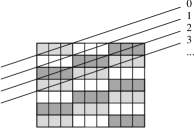
Figure 3: A series of scan lines for a given angle.

and let the lines cover such a range, that, together, they cover the entire area of the image. An example case for $a_{1}\leq\pi/4$ is illustrated in Fig. 3. As it can be seen, such a way of aligning subsequent lines provides that all pixels are covered, in scans for each $a_{1}$. Yet, there is not a separate searching for ‘bumps’ around each pixel at an angle $a_{i}$ – sequential searching for ‘bumps’ on a single line at an angle $a_{i}$ covers searching for ‘bumps’ for each pixel on that line, what decreases the mentioned computational complexity. The value of $N=7$ was chosen, as a precise enough and making the scanning reasonably fast at the same time.

The ‘bump’ criterion is as follows. Let $p_{0},\,p_{1},\,\ldots\,p_{M-1}$ be intensities of subsequent pixels on a given scanned line of $M$ pixels. The searching for ‘bumps’ within a single line works as follows: for the pixel $n$th, if its intensity is larger by $d$ than both the intensity of the pixel $(n-r)$th and the intensity of the pixel $(n+r)$th, then increase the ‘peakiness’ of the pixel by 1. The coefficients $d$ and $r$ should be large enough to reduce single–pixel level noise, and small enough to maintain good edge location. To improve the detection of edges at various scales, $p_{\max}=3$ passes of the edge detection are performed, each modifying common ‘peakiness’ of a pixel, with three different sets of values for $d$ and $r$:

$$\begin{array}[]{c}p=1,2,\ldots p_{\max}\\ r_{p}=p+2\\ d_{p}=0.015+0.005p\\ \end{array}$$ (2)

where the index $p$ denotes a respective pass. If the image processed is very blurry, $r$ might require an appropriate increase.

Because $p_{\max}N>1$ scanning lines pass through each pixel, one for each angle, the ‘peakiness’ is an averaged value of several tests for the ‘bumps’, what may obviously reduce single–pixel level noise.

Only pixels whose accumulated peakiness value is equal or larger than a given threshold $e_{\min}$ are regarded as the edge ones, to reduce the detection of what is an image noise, and not a real edge. The value of $e_{\min}=6$ was adjusted in tests. It can be decreased for images with low noise and weak edges, and increased for images with high level of noise.

The roof edges obtained using this method can be thick, while the needed edges must be one–pixel wide. To correct that, centers of the roof edges are extracted using a simple thinning method, for example that described in [3], with the 8–neighborhood criterion.

3.2 Correction of the edges

The discussed distortions, the edge detection method itself, or image noise may decrease the quality of the obtained edges. Therefore, cleaning of the edges from small branches and protruding pixels, and the reduction of ‘waving’ of the edges, is used.

3.2.1 Cleaning the edges

Both the method of the waving reduction, and the finding of approximately straight fragments discussed later in Sec. 4, are sensitive to two kinds of ‘noise’ of the edges – small branches and single protruding pixels. Example of such distortions is shown in Fig. 4. The work–around is straightforward – edges below a given length are deleted, where each pixel connecting three or more branches is considered a boundary between the edges. In the first iteration, edges of the length of $1$ are deleted, then edges of the length $2$, and so on, till some value $L_{\min}-1$, with re–measuring of the edge lengths after each iteration. If, instead, we’d immediately begin with deleting all edges of length less or equal than $L_{\min}$, then the edges like the grayed one in Fig. 4 would be deleted, instead of only the two small branches visible in the image.

The small protruding single pixels, like that seen in Fig. 4, are moved back to the edge, using a trivial method.

Figure 4: Example edge ‘noise’ to be cleaned.

3.2.2 Reduction of waving

Aliasing in the upsampled image may produce variously ‘waving’ edges, An example of ‘waving’, and its correction, is shown in Fig. 5. The edge detector should be resistant to the aliasing artifacts, thus, the reduction of the waving is performed.

Figure 5: An example of the reduction of waving for an image with two different gray response curves.

The procedure to reduce waving has the following steps:

1. Find junctions, that is corners of pixels that have two neighboring edge pixels.

2. For each of these two pixels, find the length of rectangular sequences $S$ that begin at the subsequent edge pixel. A rectangular sequence is a sequence of 4–neighboring pixels that is either vertical or horizontal.

3. If one of these cases occurs: both rectangular sequences $S$ are horizontal, or both are vertical, one consists of a single pixel and the other has more than one pixel, then such a junction can be classified as, accordingly, either horizontal or vertical. In such a case, then, it is assumed that the junction is a part of some edge $E$ that can, respectively, be classified as being locally either closer to some horizontal or vertical direction.

4. if $E$ could be classified as locally closer to horizontal or vertical direction, the junction is marked as a movable one along that closer direction, that is, able to modify $E$, by shortening the longer $S$ and extending the shorter $S$, as it is shown in the example in Fig. 6.

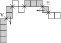
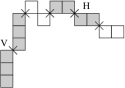
   (a)	(b)

   Figure 6: (a) Examples of junctions. The edge pixels are marked with rectangles. All junctions are marked with crosses. Only two junctions, for clarity, have their sequences $S$ marked with gray color. Possible moving direction of these two junctions are marked with arrows. The junction $H$ is the horizontal one, and the junction $V$ is the vertical one. (b) The same edge, the junctions $H$ and $V$ were moved by the length of one pixel.

5. For each movable junction, set the maximum length $l_{\max}$ the junction is allowed to move. This constraint exists to prevent the edges from too large moves. Let the two rectangular sequences $S$ neighboring to a junction have their respective lengths $s_{1}$ and $s_{2}$. Then,

   $$l_{\max}=\min\big{[}\max\left(s_{1},s_{2}\right),\,l_{1}\min\left(s_{1},s_{2}\right)+l_{2}\big{]}$$ (3)

   The basic limitation in (3) is that $l_{\max}\leq\max\left(s_{1},s_{2}\right)$, thus, an approximately straight edge can not be moved aside by more than about one pixel. The coefficients $l_{1}$ and $l_{2}$ precisely regulate $l_{\max}$. It was found in tests, that $l_{1}=3$ and $l_{2}=1$ gives a good trade–off between effective waving reduction and a none to moderate displacement of the edges.

6. After $l_{\max}$ was determined for each movable junction, the following sub–procedure $W$ is repeatedly performed, each time for the whole image, until either the number of the repetitions of performing $W$ reaches a given number $N_{w}=50$, or the stability is reached, that is a given run of $W$ does not change anything in the image. The limitation by using $N_{w}$ is only to prevent the wave reduction from taking too long time.

   $W$ is as follows. For each movable junction, if $|s_{1}-s_{2}|>1$, and the junction did not reach its $l_{\max}$ value, move the junction so that to shorten its larger sequence $S$ by one pixel and extend its shorter sequence $S$ by one pixel. The condition $|s_{1}-s_{2}|>1$ exists to cause the rectangular sequences $S$ to have more similar length, with the prevention of a junction to be moved back and forth in subsequent executions of the procedure $W$.

4 Frequency filtering

The frequency filtering has two stages: in the first stage, find approximately straight fragments of edges, and in the second stage, do frequency filtering directed along each such a fragment. Because the fragments are approximately straight, a common approximate base period of aliasing artifacts can be determined for each fragment. Such a base period $l_{0}$ is used then in filtering the frequency spectrums.

4.1 Finding approximately straight fragments

An approximately straight fragment $F$ is an edge or a part of the edge. A fragment $F$ can not include the branch pixels, that is those that have more than two neighbors being edge pixels. The criterion of a fragment to be approximately straight is very simple: all pixels of the fragment must not be further from the straight line between two endings of $F$ by more than $d=s_{d}U$. $U$ is the scale of upsampling, and it occurs in the formula because image features are linearly proportional to $U$, and $s_{d}$ is a coefficient regulating how approximately straight $F$ should be. It was determined in tests that the value of $s_{d}=0.4$ is a good trade–off between many short fragments for small $s_{d}$ and bad approximation of common $l_{0}$ for the whole $F$ for large $s_{d}$. There is yet another condition, $Q$, for $F$: its subsequent pixels must all either have always increasing or always decreasing $x$ coordinates or $y$ coordinates. If the condition applies to the $x$ coordinates, the fragment $F$ is called a horizontal one, and otherwise it is called the vertical one. An example of a horizontal $F$ is shown in Fig.7. The need for the condition $Q$ will be explained in Sec. 4.2.

The fragments $F$ are searched for as follows: find an edge pixel $P$ that is a part of an edge whose pixels are not assigned to any fragment $F$ yet. Trace the unassigned edge pixels from the pixel $P$, using the 8–neighborhood criterion, the same that was used during thinning of the edges. Do that until the end of the unassigned edge pixels is found, or a branch pixel is found. Then trace the pixels back to search for the other end of these unassigned pixels, until the other end is reached or the criterion of approximate straight edge stops to be fulfilled, and this way find a new $F$. Then set the pixels of the new $F$ as ones assigned to $F$, and continue searching for fragments $F$ until all pixels, excluding the branch pixels, are assigned to some $F$.

4.2 Fragment-directed frequency filtering

It is important for the frequency filtering to be applied possibly along object boundaries. Applying it, for example, across fence pales, may alter important image matter, as the periodicity of occurring of the pales might be confused with aliasing. This is why the edge detector is employed, and then the fragments $F$ are extracted.

With each $F$, the filtering strength $S_{f}$ is estimated. $S_{f}$ is directly related to the size of the region along $F$ that is filtered, as illustrated in Fig. 7 – the fragment is moved $S_{f}$ times up and $S_{f}$ times down for horizontal $F$, or $S$ times left and $S$ times right for vertical $F$. For each of the resulting placements, the brightness of subsequent pixels in the upsampled image, covered by the moved $F$, is determining the brightness functions $B^{b}_{i}(x)$, $x=0,\,\ldots\,N_{B}-1$, where $N_{B}$ is the number of pixels in $F$ and $i=-S_{f},-S_{f}+1,\,\ldots\,S_{f}$ is assigned for each move of $F$ as shown in the example in Fig. 7, The index $b=0,1,\,\ldots\,c-1$ determines one of the $c$ bands of the upsampled image. Each of these functions is subject to frequency filtering as described in the next section.

Figure 7: An example of a region filtered along a fragment. The fragment is marked black.

The pixels across different $i$ do not overlap, that is the band within each pixel is frequency filtered once, thanks to the condition $Q$ described in Sec. 4.1.

The variability of $S_{f}$ comes from the presume that an aliasing artifact is better detectable if it has the size of at least several lengths of $l_{0}$. It is because the artifact might be otherwise too easily mistaken with something that is not such an artifact. For example a region being a normal image matter without any artifacts might likely have the brightness that is approximately given by a fragment of a single lobe of the sine function that has the period of $l_{0}$, yet it might be much less likely that the brightness of that region is approximately given by as much as several lobes of such a sine function.

The formula for computing $S_{f}$ on basis on the number of pixels $N_{B}$ in $F$ is as follows:

$$S_{f}=\left\{\begin{array}[]{ll}\displaystyle 0&\textrm{if $N_{B}<s_{l}l_{0}$}\\ \displaystyle s_{u}N_{B}&\textrm{if $N_{B}\geq s_{l}l_{0}$}\\ \end{array}\right.$$ (4)

As it can be seen, $S_{f}=0$ if the fragment is too short, to decrease the probability of confusing an artifact with image matter, as discussed earlier in this section. Otherwise, $S_{f}$ gradually increases with $s_{u}N_{B}$. The coefficients $s_{l}$ and $s_{u}$ were tuned in a series of tests. Small $s_{l}$ means a greater probability of an undesired distortion caused by the frequency filtering of image objects that are not artifacts. Conversely, large $s_{l}$ means that more artifacts might be left uncorrected. The coefficient $s_{u}$ regulates the strength of $S$, which in turn is connected with the range along $F$ that is filtered. Thus, small $s_{u}$ means that an artifact might be corrected only in its small part closer to $F$, and large $s_{u}$ means that some regions lying further to $F$ might be undesirably distorted by the filtering. It was found experimentally, that $s_{l}=2$ and $s_{u}=0.25$ give relatively good results.

4.3 Filtering of the brightness function

The FFT requires the transformed function to have the number of pairs to be the power of 2, what is untrue in general for $B^{b}_{i}(x)$. To prevent spurious high frequency components and to fulfill the requirement for the number of pairs, $B^{b}_{i}(x)$ is padded with additional elements to create $C^{b}_{i}(x)$. Let the number of pairs in $C^{b}_{i}(x)$ be such a smallest possible value $N_{C}$ that it is the power of 2 and the number of pad pairs $N_{C}-N_{B}$ to add to $B^{b}_{i}(x)$ to create $C^{b}_{i}(x)$ is greater than or equal to $\lfloor N_{B}/2\rfloor$, Let the mean value of $B^{b}_{i}(x)$ be $t^{b}_{i}$. The function $C^{b}_{i}(x)$ is defined as follows:

$$\begin{array}[]{c}x=0\ldots N_{C}-1\\ m_{C}=\lfloor(N_{C}-N_{B})/2\rfloor\\ e_{C}=\lfloor m_{C}+N_{B}-1\rfloor\\ w_{l}=x/(m_{C}-1)\\ w_{r}=(N_{C}-1-x)/(N_{C}-2-e_{C})\\[8.0pt] C^{b}_{i}(x)=\left\{\begin{array}[]{ll}w_{l}B^{b}_{i}(m_{C}-x)+(1-w_{l})t^{b}_{i}&\textrm{for $x<m_{C}$}\\ B^{b}_{i}(x-m_{C})&\textrm{for $x\geq m_{C}\,\land$}\\ &\textrm{$x\leq e_{C}$}\\ w_{r}B^{b}_{i}(2e_{C}-x)+(1-w_{r})t^{b}_{i}&\textrm{for $x>e_{C}$}\\ \end{array}\right.\par\end{array}$$ (5)

Thus, there are two mirror margins added with their widths of at least $\lfloor N_{B}/4\rfloor$ each, that converge to the mean value of $B^{b}_{i}(x)$ at the lowest and the highest arguments of $C^{b}_{i}(x)$. The requirement for minimum width of the margins and the common convergence value minimize spurious high frequency components in the spectrum of $C^{b}_{i}(x)$. There is an example of the function $C^{b}_{i}(x)$ in Fig. 8.

Figure 8: An example of the functions $C^{b}_{i}(x)$ and $C^{\prime b}_{i}(x)$. Their fragments from index 18 to index 44 are exact repetitions of, respectively, $B^{b}_{i}(x-18)$ and $B^{\prime b}_{i}(x-18)$.

Let the brightness function $C^{b}_{i}(x)$ after transforming it with the FFT be $F^{b}_{i}(f)$, $f=0,\ldots\,N_{C}-1$. Because $C^{b}_{i}(x)$ is real, it holds true that $F^{b}_{i}(f)=F^{b}_{i}(N_{C}-1-f)$ for the whole domain of $F^{b}_{i}(f)$. Further, because of that symmetry, each operation to $F^{b}_{i}(f)$ will also implicitly be applied to $F^{b}_{i}(N_{C}-1-f)$, and charts will show $F^{b}_{i}(f)$ only for $f=0,\ldots\,N_{C}/2-1$. Let $f_{0}=N_{C}/l_{0}$ be the frequency corresponding to $l_{0}$. If $B^{b}_{i}(x)$ contains aliasing, peaks are expected near to $f_{0}$ and its harmonics in $F^{b}_{i}(f)$. Because altering only the peak at $f_{0}$ appeared to be very effective, the peaks at harmonics of $f_{0}$ are ignored. Simply setting the values of $F^{b}_{i}(f)$ at or near $f_{0}$ to 0 might produce the valley that would distort fragments that do not have any artifacts, because a valley might appear in the frequency spectrum where there was not even any peak resulting from the aliasing. The solution is to compute the mean $m$ around the expected peak at $f_{0}$, and if the modulo of peak values exceed $m$, flatten the peak down to the mean $m$. The mean $m$ is weighted using the weight function $W(f)$ such that it has its maximum values at approximately $1/2$ and $3/2$ of $f_{0}$, and thus, these regions of maximum values are placed away from both $f_{0}$ and the harmonics of $f_{0}$, which in turn could contain peaks resulting from the aliasing, and thus skew the value of $m$. The corresponding formulas for computing $m$ are as follows:

$$\begin{array}[]{c}\displaystyle\begin{array}[]{rl}\displaystyle W(f)=&1/\big{[}1+w_{s}(f-\frac{1}{2}f_{0})^{2}\big{]}+\\[6.0pt] &1/\big{[}1+w_{s}(f-\frac{3}{2}f_{0})^{2}\big{]}\\[6.0pt] \end{array}\\ \displaystyle S=\sum_{f=0}^{f<N_{C}}W(f)\\[16.0pt] \displaystyle m=\frac{\sum_{f=0}^{f<N_{C}}W(f)F^{b}_{i}(f)}{S}\end{array}$$ (6)

The coefficient $w_{s}$ determines the width of each of the two peaks and was tuned to 3 using test images. The value $S$ is computed to normalize the weight function $W(f)$. An example diagram of $W(f)$ is shown in Fig. 9.

Figure 9: An example of filtering of a function $B^{b}_{i}(x)$ from Fig. 8. The functions $W(f)$ and $M(f)$ are so distorted because of the low value of $N_{C}$.

The reduction of the peak is in detail performed as follows. Firstly, let the peak be located by a function $M(f)$. The value of the function is interpreted as follows: $1$ for no altering of the spectrum at $f$, $0$ for a maximum altering of the frequency spectrum at $f$, that is, lowering its modulo values to $m$ if greater, Values of $M(f)$ in between $0$ and $1$ determine respective partial alteration. The function $M(f)$ is computed as follows:

$$M(f)=\left\{\begin{array}[]{ll}1&\textrm{if $f=0$}\\ \tanh\left[m_{s}\left(N_{C}/f-l_{0}\right)^{2}\right]&\textrm{if $f>0$}\\ \end{array}\right.$$ (7)

The function is constructed so that $M(f)$ creates a valley at and near the peak with the lowest value close to $0$, is equal to $1$ at the constant component $f=0$, almost equal to $1$ for frequencies substantially lower or higher than $f$. The coefficient $m_{s}=0.03$ was tuned to regulate the width and slopes of the valley. The limited steepness of the slopes of $M(f)$ reduces the the possible distortions in the space domain caused by the frequency filtering. The left slope is so steep to decrease the reduction of low frequencies. Reducing them, because of their usually large values, appeared to produce strong discontinuity effects between the filtered region and the rest of the image.

The discussed alteration of $F^{b}_{i}(f)$ so that it creates $F^{\prime b}_{i}(f)$ has the following equation:

$$\forall_{f}\quad|F^{\prime b}_{i}(f)|=\left\{\begin{array}[]{ll}M(f)|F^{b}_{i}(f)|+&\\ \quad+\big{[}1-M(f)\big{]}m&\textrm{if $|F^{b}_{i}(f)|>m$}\\ |F^{b}_{i}(f)|&\textrm{if $|F^{b}_{i}(f)|\leq m$}\\ \end{array}\right.$$ (8)

An example of filtering of $F^{b}_{i}(f)$ is shown in Fig. 9. The function $F^{\prime b}_{i}(f)$ is transformed using reverse FFT into $C^{\prime b}_{i}(x)$, from which is extracted $B^{\prime b}_{i}(x)=C^{\prime b}_{i}(x-m_{C})$, $x=0\,\ldots\,N_{B}-1$, to remove the padding introduced in (5). $B^{\prime b}_{i}(x)$ is thus a frequency–filtered $B^{b}_{i}(x)$, and is written back to the upsampled image, to the exact pixels from which $B^{b}_{i}(x)$ was constructed.

5 Tests

An example image processed with the presented method is shown in Fig. 10(d). The image was upsampled four times using bicubic interpolation that employed Catmull–Rom spline [9]. The edge map of the image is shown in Fig. 10(b). As it can be seen, the image with reduced aliasing is visually radically improved over the image obtained using plain upscaling without the frequency filtering, shown in Fig. 10(c). The aliasing in Fig. 10(d) is almost reduced, without any substantial blur, loss of small details or other distortions visible. It differs the presented method from that of an anisotropic smoothing [12] shown in Fig. 11, which, while reducing the aliasing, distorts the image so that it looks very unnatural and blurred. For example, most of the details in the center of the petal in Fig. 11 are almost lost.

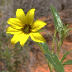
(a)	(b)
(c)	(d)

Figure 10: An example of filtering a photograph: (a) original image, (b) subpixel precision edges found, thickened in the illustration to make them better visible, (c) upsampled image without the frequency filtering, (d) upsampled image with the frequency filtering.

Figure 11: The image from Fig. 10(a) upsampled using a GREYC anisotropic smoothing.

It can be seen in the image, that the introduced method works well for various non–straight curves, even that it splits them into the approximately straight fragments before the frequency filtering.

6 Conclusion

The presented method can be applied to images upsampled using different interpolation method, and can radically reduce aliasing, with a very good preservation of the rest of the filtered image. The method has the side effect of producing a subpixel precision edge map, that can be used in various edge processing algorithms, like the sharpening of edges in the upsampled image, for further improvement of its quality.

References

- [1] S. Baker, S. K. Nayar, and H. Murase. Parametric feature detection. International Journal of of Computer Vision, 27(1):27–50, 1998.
- [2] J. Canny. A computational approach to edge detection. IEEE Trans. Pattern Analysis and Machine Intelligence, 8:679–698, 1986.
- [3] R. C. Gonzales and R. E. Woods. Digital Image Processing. Addison Wesley, 1993.
- [4] A. Jain. Fundamentals of Digital Image Processing. Prentice-Hall, 1989.
- [5] R. Keys. Bicubic interpolation. IEEE Trans. Acoust. Speech, Signal Processing, 29:1153–1160, 1981.
- [6] Xin Li. New edge–directed interpolation. IEEE Transactions on Image Processing, 10(10):1521–1527, 2001.
- [7] D. Marr and E. C. Hildreth. Theory of edge detection. In Proc. Royal Soc. London, B 207, pages 187–217, 1980.
- [8] D. Martin, C. Fowlkes, and J. Malik. Learning to detect natural image boundaries using local brightness, color and texture cues. IEEE Transactions on Pattern Analysis and Machine Intelligence, 26(5):530–541, 2004.
- [9] D. P. Mitchell and A. N. Netravali. Reconstruction filters in computer graphics. In Proceedings of the 15th annual conference on Computer graphics and interactive techniques, pages 221 – 228, 1988.
- [10] P. Perona and J. Malik. Detecting and localizing edges composed of steps, peaks, and roofs. Technical report, MIT, 1991.
- [11] I. Sobel. Camera Models and Machine Perception. PhD thesis, Stanford University, U.S.A., 1970.
- [12] D. Tschumperle. Fast anisotropic smoothing of multi-valued images using curvature-preserving pde’s. International Journal of Computer Vision, 68(1):65–82, 2006.
- [13] D. Tschumperle and R. Deriche. Vector-valued image regularization with pde’s: A common framework for different applications. IEEE Transactions on Pattern Analysis and Machine Intelligence, 27(4):506–517, 2005.
- [14] D. Ziou and S. Tabbone. Edge detection techniques - an overview. International Journal of Pattern Recognition and Image Analysis, 8:537–559, 1998.