A robust solution procedure for hyperelastic solids with large boundary deformation

Abstract

Compressible Mooney-Rivlin theory has been us-
ed to model hyperelastic solids, such as rubber and porous polymers, and more recently for the modeling of soft tissues for biomedical tissues, undergoing large elastic deformations. We propose a solution procedure for Lagrangian finite element discretization of a static nonlinear compressible Mooney-Rivlin hyperelastic solid. We consider the case in which the boundary condition is a large prescribed deformation, so that mesh tangling becomes an obstacle for straightforward algorithms. Our solution procedure involves a largely geometric procedure to untangle the mesh: solution of a sequence of linear systems to obtain initial guesses for interior nodal positions for which no element is inverted. After the mesh is untangled, we take Newton iterations to converge to a mechanical equilibrium. The Newton iterations are safeguarded by a line search similar to one used in optimization. Our computational results indicate that the algorithm is up to 70 times faster than a straightforward Newton continuation procedure and is also more robust (i.e., able to tolerate much larger deformations). For a few extremely large deformations, the deformed mesh could only be computed through the use of an expensive Newton continuation method while using a tight convergence tolerance and taking very small steps.

1 The problem under consideration

We consider the problem of solving for the deformed shape of a hyperelastic solid body under static loads. The continuum mechanical model under consideration has the following description Holzapfel . Let $B_{0}\subset{\bf R}^{d}$ be an undeformed solid body whose boundary is $\partial B_{0}$. Here $d$, the space dimension, is 2 or 3. Assume boundary conditions (either displacement or traction, i.e., Dirichlet or Neumann) are given as follows. The boundary $\partial B_{0}$ is partitioned into two subsets $\Gamma_{D}$ and $\Gamma_{N}$. A function $\phi_{0}\mbox{:}\Gamma_{D}\rightarrow{\bf R}^{d}$ specifies new-position (Dirichlet) boundary conditions. A second function ${\bf t}_{0}\mbox{:}\Gamma_{N}\rightarrow{\bf R}^{d}$ specifies traction (Neumann) boundary conditions. Everything in this paper extends to the more general case that some coordinate entries are Neumann while others are Dirichlet at certain boundary points, but we limit the discussion to the special case that each boundary point is Dirichlet or Neumann in all $d$ coordinates in order to simplify notation. Finally, the model requires a specification of the model’s body forces, that is, a function $\mathbf{b}\mbox{:}B_{0}\rightarrow{\bf R}^{d}$ that specifies the force of gravity and other forces on the body.

The problem is to find a function $\phi\mbox{:}B_{0}\rightarrow{{\bf R}}^{d}$ that specifies the new position of the body. Let $B$ denote $\phi(B_{0})$. For a point ${\bf X}\in B_{0}$, let ${\bf x}=\phi({\bf X})$. Let $F$ be the deformation gradient, i.e., $F=d\phi/d{\bf X}=d{\bf x}/d{\bf X}$. It is assumed that $F({\bf X})$ has a positive determinant for all ${\bf X}$. The Green-Lagrange strain tensor is defined to be $E=(F^{T}F-I)/2$. Let scalar function $\Psi(F)$ be the strain energy function, which is assumed to be a property of the material. For this paper, we assume that $\Psi$ depends only on two scalar invariants of tensor $E$, namely $J=\det(F)=\sqrt{\det(2E+I)}$ and $I_{1}=\mbox{trace}(F^{T}F)=\mbox{trace}(2E+I)$. Further specializing the model, the strain energy is then taken to have the following form suggested by Ciarlet and Geymonat in Ciarlet for compressible Mooney-Rivlin materials

$$\Psi(F)=\frac{\lambda}{4}(J^{2}-1)-\left(\frac{\lambda}{2}+\mu\right)\ln J+\frac{\mu}{2}(I_{1}-3)$$ (1)

where $\lambda,\mu>0$ are material parameters. Compressible Moo-
ney-Rivlin theory has been used for analyzing large elastic deformations of soft materials, including rubber mooney_rivlin_original ; porous polymers, such as porous polyethylenes used as insulation boards for construction, protective packaging materials, insulated drinking cups, and flotation devices gibson_ashby ; and biological tissues weichert ; as well as other applications.

For the $d=2$ case, we assume that $B_{0}$ is 3D but that the $z$-displacement is identically $0$ and that the $x$- and $y$-displacements depend only on $x$ and $y$; these are called plane strain assumptions. Thus, $E$ has a last row and column of all zeros, and the Mooney-Rivlin formula in $(\ref{eq:MR-model})$ is applied to this $E$ to come up with the strain energy function for the $d=2$ case. The condition for static equilibrium (written in minimization form) is that

$$\int_{B_{0}}\Psi(F({\bf X}))\,dV-\int_{B_{0}}\rho\mathbf{b}\cdot\phi({\bf X})\,dV-\int_{\Gamma_{N}}{\bf t}_{0}\cdot\phi({\bf X})\,dA$$ (2)

is minimized among all choices of $\phi$ that satisfy the Dirichlet boundary condition, i.e., that satisfy $\phi({\bf X})=\phi_{0}({\bf X})$ for all ${\bf X}\in\Gamma_{D}$.

This condition can be rewritten in variational form: for all admissible variations $\delta{\bf u}$, that is, functions in the space $[H^{1}(B_{0})]^{d}$ that vanish on $\Gamma_{D}$,

$$\int_{B_{0}}\frac{\partial\Psi}{\partial F}\mbox{:}\mbox{Grad}\ \delta{\bf u}\ dV-\int_{B_{0}}\rho\mathbf{b}\cdot\delta{\bf u}\,dV-\int_{\Gamma_{N}}{\bf t}_{0}\cdot\delta{\bf u}\,dA=0,$$ (3)

where $A\mbox{:}B=\mbox{trace}(AB^{T})$ is used to denote the inner product of second-order tensors $A$ and $B$. This model also applies to the case of linear elasticity with two changes in definitions. First, $E=((F-I)^{T}+(F-I))/2$ in the case of linear elasticity. Second, $\Psi=\mu\sum_{i,j}E(i,j)^{2}+\frac{\lambda}{2}\left(\sum_{i}E(i,i)\right)^{2}$, which can be written in terms of the two invariants of $E$.

We should mention that our method does not appear to depend so much on the specific details of the Mooney-Rivlin model, except for the $\ln J$ term, which is quite important for our analysis. Since $dv=J\,dV$, where $dv$ is the volume element of $B$ and $dV$ is the volume element of $B_{0}$, this logarithmic term resists infinite compression of the material: if a small positive volume of material in $B_{0}$ shrinks to a 0-volume set in $B$, then this term causes the strain energy at those points to become infinite.

We next describe the Lagrangian discretization of the problem under consideration BelytschkoLiu . We assume that $B_{0}$ is discretized with a mesh of triangles or tetrahedra. We assume that the discretization of $\phi$, or alternatively the discretization of the displacement ${\bf u}=\phi({\bf X})-{\bf X}$, is piecewise linear, with the pieces of linearity being the mesh cells. (In Section 8, we discuss extension of our method to piecewise quadratic displacements.) Recall that $d$ is the space dimension, and let $m$ denote the number of non-Dirichlet nodes of the mesh. This assumption implies that ${\bf u}$ is determined by $dm$ real numbers, namely, the values of ${\bf u}$ at nodes. The finite element method finds the displacement ${\bf u}$ such that $(\ref{eq:varform})$ holds for all test functions $\delta{\bf u}$ in the test function space. Here, the test function space is the set of $\delta{\bf u}$’s that are piecewise linear and continuous and vanish on $\Gamma_{D}$. The integral in $(\ref{eq:varform})$ is evaluated with a quadrature rule; we have used a 6-point formula having degree 4 precision from Hughes for our quadrature in 2D and a 15-point formula having degree 5 precision from Keast for 3D. It suffices to solve $(\ref{eq:varform})$ for the $dm$ choices of $\delta{\bf u}$ that compose the standard basis for the test function space. This yields a system of $dm$ nonlinear equations for $dm$ unknowns.

The algorithmic question under consideration is how to robustly solve these nonlinear equations. In the next section, we give a summary of the mesh tangling issue and of our proposal to overcome it. The individual steps of our algorithm are then described in more detail in Sections 4 and 5. In Section 3, we summarize the Newton continuation algorithm which is a popular technique within the engineering community for solving the nonlinear equations. Our computational experiments, which compare the two algorithms, are presented in Sections 6 and 7. Concluding remarks, including some discussion of the incompressible case, are presented in Section 8.

The preceding formulation is called “Lagrangian” discretization because the nodes of the mesh remain fixed with respect to material points throughout the solution procedure. Alternatives to the Lagrangian approach include the Eulerian approach and arbitrary Lagrangian-Eulerian (ALE) methods. Pure Eulerian methods are not widely used in solid mechanics because of the difficulty in applying boundary conditions. ALE methods are a more viable competitor to Lagrangian methods; in ALE methods the geometry is reme-
shed as part of the solution procedure. ALE remeshing attempts to preserve a high-quality mesh as the solution evolv-
es. ALE methods are substantially more complicated than Lagrangian methods because of the need to interpolate field quantities to new mesh points on every remeshing step. In addition, ALE remeshing is itself somewhat of an art in that there is no foolproof universal procedure for updating the mesh.

For these reasons, we focus on traditional Lagrangian solution techniques in this paper. Nonetheless, the first part of our algorithm (called “iterative stiffening” in Section 4) can be regarded as a particular ALE remeshing approach; we return to this topic later.

2 Mesh tangling

The standard method for solving a system of nonlinear equations is Newton iteration. It is well-known, however, that if the initial guess is far from the true solution, then Newton iteration will often diverge.

In the case of hyperelasticity with large deformation, there is a specific obstacle that may cause divergence, namely, mesh tangling. The definition of this term is that a mesh is tangled if the value of $J$ defined in the previous section is 0 or negative in $B_{0}$. In the case of linear displacements, $J$ is piecewise constant, and hence this condition can be verified with a finite number of determinant computations. The matter of checking for tangling in the piecewise quadratic case is more complicated and is discussed in Section 8. A solution with a tangled mesh is physically invalid. Indeed, the strain energy function is undefined in this case because of the presence of the term $-\left(\frac{\lambda}{2}+\mu\right)\ln J$. Note that although the strain energy function is undefined when $J$ is negative, the Galerkin form $(\ref{eq:varform})$ is still well defined, which is an anomaly that we return to below. We assume that the given problem instance has a valid solution, i.e., there is a piecewise linear function ${\bf u}$ satisfying the boundary conditions, as well as $(\ref{eq:varform})$ for all test functions $\delta{\bf u}$ plus the condition that $J>0$ on every element.

Even with this assumption, Newton’s method will still often run into problems because the mesh will become tangled on intermediate steps. For example, the starting point for Newton’s method is often taken to be ${\bf u}={\bf 0}$ on every interior node. If the deformation of the boundary is large, then this starting point corresponds to a mesh which will have tangling among most of the elements that are adjacent to the boundary.

To understand a difficulty posed by a tangled mesh, suppose that the strain energy has a single term

$$\Psi(J)=-\left(\frac{\lambda}{2}+\mu\right)\ln J$$

(for $\frac{\lambda}{2}+\mu>0)$ on a single element and that there are no boundary constraints. If we treat $J$ as the independent scalar variable, then Newton’s method for minimizing this scalar function is

$$J^{(i+1)}=J^{(i)}-\Psi^{\prime}(J^{(i)})/\Psi^{\prime\prime}(J^{(i)})$$

which simplifies in this case to

$$J^{(i+1)}=2J^{(i)}.$$

For positive $J^{(0)}$, this iteration produces a sequence of $J$’s tending to $+\infty$. This is to be expected since the minimum of $-\left(\frac{\lambda}{2}+\mu\right)\ln J$ is indeed at $+\infty$. On the other hand, for a negative $J^{(0)}$, this iteration tends to $-\infty$, which is physically invalid.

The preceding analysis, although naive, seems to point to the following conclusion: Newton’s method on the Galer-
kin form, when applied to a tangled mesh, has a natural tendency to make the tangling worse. We suspect that this fact is probably already known to experts in the field, although we have not been able to find it in the previous literature.

Given the conclusion in the previous paragraph, it seems of paramount importance to avoid tangling. When Newton’s method fails in computational mechanics, it is standard practice to try Newton continuation, that is, to apply the load in incremental steps and use the converged solution for one step as the Newton starting point for the next step. Continuation is described in more detail in Section 3. Continuation, however, addresses the tangling issue only in an indirect fashion and therefore is likely to be very inefficient. Our computational experiments confirm the inefficiency of continuation.

We propose a new algorithm for getting around the mesh tangling obstacle. The basic idea is to first untangle the mesh using a much simplified mechanical model. Once the mesh is untangled, the true mechanical model is solved. “Untangling the mesh” means finding a $\phi$ that satisfies the Dirichlet boundary condition and also satisfies $J>0$. Our new algorithm, which we call UBN (for “untangling before Newton”) consists of two steps.

1. First, we attempt to untangle the mesh with the iterative-stiffening algorithm, described in Section 4. Iterative stiffening builds on the FEMWARP algorithm from our previous work ShontzVava . That paper, however, concerned itself with a pure mesh generation problem (devoid of physics), whereas, in this work, the topic is solving a classical nonlinear boundary value problem in mechanics. If the iterative stiffening algorithm cannot untangle the mesh, then UBN reports failure to solve the problem.

2. Else if iterative stiffening succeeds, then we take Newton iterations to solve $(\ref{eq:varform})$. The starting point for Newton is an untangled mesh produced by step 1. No continuation is used. On the other hand, Newton’s method is safeguarded using a line search described in Section 5, which prevents the introduction of new tangling. The line search is based on a technique common in the interior point literature (see e.g., wright_ipm ).

3 Newton continuation

In the case that direct use of Newton’s method to find $\phi$ fails to converge, the standard alternative is Newton continuation, also known as applying the load in steps. This section briefly describes Newton continuation before we return to a description of UBN.

The basic form of Newton continuation is quite straightforward: a sequence of parameters $0=\tau_{0}<\tau_{1}<\cdots<\tau_{N}=1$ is chosen, and a sequence of displacement vectors ${\bf u}_{0},{\bf u}_{1},$
$\ldots,{\bf u}_{N}$ is computed, in which for each $k$, ${\bf u}_{k}$ is the solution to the discretized $(\ref{eq:varform})$ in the case that $(\phi_{0}({\bf X})-{\bf X},\mathbf{b},{\bf t}_{0})$ are replaced by $\tau_{k}\cdot(\phi_{0}({\bf X})-{\bf X},\mathbf{b},{\bf t}_{0})$. Solution ${\bf u}_{0}$ (corresponding to absence of loads) is identically ${\bf 0}$. (In the case that additional information is available about the final solution, one might be able to formulate a better initial guess for ${\bf u}$; however, ${\bf u}_{0}={\bf 0}$ is the default value for most continuation codes.) Solution ${\bf u}_{k}$ is found via Newton’s method, where ${\bf u}_{k-1}$ is used as the initial guess. The final deformed configuration is given by ${\bf u}_{N}$ since $\tau_{N}=1$. Note also that it is possible to accept a low-accuracy (not fully converged) solution for ${\bf u}_{k}$ when $k<N$ since it is presumably not necessary to achieve high accuracy for intermediate results that are not part of the ultimate answer.

In some cases, a straight linear parametrization of the load path (as in the previous paragraph) is not feasible. In this case, one must construct a nonlinear parametrization $(\phi_{NLP}({\bf X};\tau),\mathbf{b}_{NLP}({\bf X};\tau),{\bf t}_{0,NLP}({\bf X};\tau))$ with the property that $\phi_{NLP}({\bf X};0)={\bf X}$ while $\phi_{NLP}({\bf X};1)=\phi_{0}({\bf X})$ and similarly for the other load terms. Examples of nonlinear parametrizations are given later in the paper.

The only remaining issue is how to select the sequence of $\tau_{k}$’s. We use an adaptive rule defined as follows. Assume that there are no body forces and that the traction boundary conditions are all zero (i.e., “traction-free” surfaces). This means that the only loading term is the Dirichlet boundary condition. We form the deformed mesh $M_{k-1}$ after applying the displacements given by ${\bf u}_{k-1}$ to non-Dirichlet nodes and Dirichlet boundary conditions scaled by $\tau_{k-1}$, (i.e., the deformed position is given by ${\bf X}+\tau_{k-1}(\phi_{0}({\bf X})-{\bf X})$ in the case of linear parametrization) to Dirichlet nodes. Next, we compute a value of $\tau_{k}$ such that, if the boundary nodes in $M_{k-1}$ are further deformed to positions given by ${\bf X}+\tau_{k}(\phi_{0}({\bf X})-{\bf X})$, then no tetrahedron altitude will decrease by more than a factor of $\eta$, where $\eta$ is a tuning parameter of the continuation algorithm. Typically $\eta\leq 1$. (In particular, the step is sufficiently small that the mesh will not tangle after the new boundary condition given by $\tau_{k}$ is applied to $M$.) We also investigate some more aggressive continuation strategies with $\eta>1$ in our experiments in Sections 6 and 7. This adaptive strategy appears to work reasonably well, although we did encounter some robustness problems discussed in Section 7. We also compare these adaptive step selection strategies with a constant step-size strategy.

In this paper, we assume that the problem under consideration is to determine a single final configuration. Newton continuation finds this final configuration, and, as a by-product, also computes many intermediate configurations. In some applications this “by-product” is in fact the principal application of continuation. For example, the entire loading path is sometimes sought when the hyperelastic material is, in and of itself, the object of study (e.g., a study of soft-tissue deformation or damage due to an impact).

On the other hand, for problems in which the hyperelastic material is merely one component of a larger problem (e.g., a vibration isolator in the model of a large structure), the entire load path is usually not needed. Furthermore, even in applications where the entire loading path is required, our technique is applicable since UBN can be used in combination with Newton continuation to obtain an improved initial guess and larger steps than is possible using Newton continuation alone.

The description in the earlier paragraphs assumed the special case of traction-free Neumann boundaries and absence of body forces. It is more difficult to use this adaptive technique when there are nonzero body forces or tractions since it is not obvious how to step these loads in a way that prevents tangling on each step. Therefore, most of our test cases focus on the traction-free case. Since the focus of the paper is the UBN method, it represents a strengthening of our contention that UBN is usually better than the competing algorithm (continuation) since we limit our testing only to the case that seems well suited for continuation. Nonetheless, we have also tried examples with nonzero tractions; we report on this experiment at the end of Section 7.

4 Iterative stiffening for mesh untangling

In this section, we describe our procedure called iterative stiffening for untangling a mesh. We take the original mechanical problem given by $(\ref{eq:varform})$, and using the same boundary conditions and loads, we solve the equations of isotropic linear elasticity using piecewise linear (constant-strain) finite elements BelytschkoLiu . Note that these equations have the same material parameters (the Lamé constants $\lambda$ and $\mu$) as the Mooney-Rivlin model. Linear elasticity requires one linear system solve. If the deformed mesh (i.e., the mesh that arises from moving the nodes to their displaced positions) is untangled, then iterative stiffening is finished. If not, then our iterative stiffening procedure locates all elements that are inverted in the deformed mesh and increases their stiffness by 50%. The linear elasticity model is now solved again. This procedure is repeated indefinitely until the mesh is untangled or an excessive number of iterations has passed.

We have not found this precise version of iterative stiffening appearing in the previous literature, but it is related to ideas already in the literature. It is closely related to “Jacobian techniques” of Stein et al. SteinTezduyarBenney . It could be regarded as an extension of FEMWARP, a finite element based mesh warping approach developed by the authors within the linear weighted Laplacian smoothing (LWLS) framework ShontzVava ; shontz-thesis . One difference is that FEMWARP does not easily encompass the mechanical concept of traction boundary conditions. It is also related to a mesh warping method used for ALE solvers and described in Chapter 7 of BelytschkoLiu .

We remark that iterative stiffening, which we treat herein as the first step of UBN, could be a standalone algorithm for ALE remeshing. Indeed, this is the application for “Jacobian techniques” mentioned above.

In our preliminary version of the UBN method shontz-thesis , the untangling was done using Opt-MS FreitagPlassmann rather than iterative stiffening. Opt-MS is an untangling algorithm that iteratively repositions interior nodes one at a time until the mesh is untangled. It solves a small linear-programming problem for each node to find the position for it that maximizes the minimum area (volume) of an element in the local submesh constructed from its neighboring triangles (tetrahedra). The area (volume) of a triangle (tetrahedron) is computed via the determinant of the Jacobian of the element. We found recently that iterative stiffening is more effective for use in UBN than Opt-MS. One possible reason is that it is difficult to implement traction boundary conditions in a natural way in Opt-MS.

Note that iterative stiffening can be made particularly efficient by using matrix-updating. In particular, it is well-known (see, e.g. GVL ) how to update a Cholesky factorization of a symmetric positive definite matrix $A$ after $A$ has undergone a low-rank update. If the iterative stiffening procedure stiffens only a few elements per iteration (our test runs confirm that indeed there are usually only a few updates per step), then this can be implemented as a a low-rank update, which is potentially much more efficient than solving a new stiffness matrix from scratch. We did not implement matrix-updating because the work for iterative stiffening was usually dominated by the solver part of the algorithm anyway.

5 Newton Line Search

Newton’s method is often employed for solving nonlinear systems of continuously differentiable equations dennis_schnabel . Let $f\mbox{:}{\bf R}^{dm}\rightarrow{\bf R}^{dm}$, continuously differentiable, be given. The task at hand is to find a ${\bf u}\in{\bf R}^{dm}$ such that $f({\bf u})={\bf 0}$. Let ${\bf u}_{0}\in{\bf R}^{dm}$ be given. Then, at each iteration $k$, Newton’s method solves

$$J({\bf u}_{k}){\bf s}_{k}=-f({\bf u}_{k}),$$ (4)

where $J$ denotes the Jacobian of $f$, for the Newton step, ${\bf s}_{k}$, and performs the following update

$${\bf u}_{k+1}={\bf u}_{k}+{\bf s}_{k}.$$ (5)

If it becomes necessary to satisfy one or more additional inequality constraints, it is possible to safeguard the Newton step with the introduction of a line search. Let $\alpha_{k}$ denote the line search parameter. Then $\alpha_{k}$ is chosen to be as large as possible such that $0<\alpha_{k}\leq 1$ and ${\bf u}_{k+1}={\bf u}_{k}+\alpha_{k}{\bf s}_{k}$ satisfies the constraint.

It is often difficult to compute the value of $\alpha_{k}$ that minimizes $f({\bf x}_{k}+\alpha_{k}{\bf s}_{k})$ and satisfies the constraint because $f$ is often a highly nonlinear function. In addition, the optimal value of $\alpha_{k}$ often produces steplengths that are too short in practice. Thus, it is common practice in interior point methods to derive heuristics for computing $\alpha_{k}$ that allow for both ease of computation and larger steplengths wright_ipm . One such heuristic is to choose $\alpha_{k}$ so as to stay a fixed percentage away from the boundary. We employ this heuristic in our line search below.

As was pointed out in Section 2, the mesh is tangled unless $J=\det(F)>0$. Thus, we introduce a line search that enforces that $J>0$ on each iteration of Newton’s method. In particular, we begin with $J>0$ on the zeroth iteration and choose the line search parameter $\alpha_{k}$ such that $J({\bf u}_{k+1})\geq 0.1J({\bf u}_{k})$ on each element so as to stay a fixed percentage away from the boundary for reasons discussed above.

The following pseudocode algorithm shows how the line search parameter is determined. Let $N$ denote the number of elements in the mesh. Given a displacement vector ${\bf u}$, it is straightforward for each element $i=1,\ldots,N$ to compute the deformation gradient $F$ and its determinant $J$ determined by this displacement on element $i$; we denote the resulting determinant by $J({\bf u},i)$.

Let ${\bf u}_{0}$ be the value of the displacement (at non-Dirichlet nodes) returned by the previous iteration of our Newton/line search algorithm. Initially, the value of ${\bf u}_{0}$ is the output of the iterative stiffening algorithm. It is assumed that the mesh determined by the Dirichlet boundary conditions and by ${\bf u}_{0}$ on non-Dirichlet nodes is untangled. Let ${\bf s}$ denote the Newton step determined from ${\bf u}_{0}$ via $(\ref{eqn:newton})$.

$\alpha=1;$
for $i=1\mbox{:}N$
	while true
		if $J({\bf u}_{0}+\alpha{\bf s},i)\geq J({\bf u}_{0},i)/10$
			break
		end
		$\alpha=\alpha\cdot 0.9;$
	end
end

6 2D Experiments

We designed a series of numerical experiments in order to test the robustness of UBN and to compare it to the standard Newton continuation algorithm. As explained in Section 3, most of our test cases involve only traction-free, body-force-free loading conditions. For all of the numerical experiments in this paper, we set the parameters in $(\ref{eq:MR-model})$ as follows: $\lambda=\frac{\nu E}{(1+\nu)(1-2\nu)}$ and $\mu=\frac{E}{2(1+\nu)}$, with $E=1$ and $\nu=0.3$.

The termination criteria for the Newton loop in UBN and for the final step of Newton continuation was that $\|F\|_{2}\leq 10^{-10}\|F_{0}\|_{2}$, where $F_{0}$ is the initial value (i.e., the value when all interior displacements are set to 0) of the load vector. For the Newton continuation steps prior to the final step, the termination criteria was that $\|F\|_{2}\leq tol\|F_{k_{i}}\|_{2},$ where $F_{k_{i}}$ is the initial value of the load vector at the beginning of major iteration $k$, and $tol=10^{-3}$ or $10^{-5}$. The looser tolerance was chosen because it was important to determine the value of the stopping criterion which makes Newton continuation as efficient as possible (for the purposes of comparison with UBN). The tighter tolerance was chosen for the purposes of improving the robustness of Newton continuation on highly deformed meshes. The algorithms were implemented in Matlab.

The linear solution operation in Matlab is quite highly optimized and is expected to compete well with a custom-written C or C++ linear solver. On the other hand, the matrix assembly process involves several nested Matlab loops and is therefore expected to be much slower than a C or C++ version. For this reason, wall-clock times derived from the Matlab code are not useful predictors of computational demands that would be observed with a C or C++ code.

Instead, we measure the running time in terms of assembly/linear solve steps. An assembly/linear solve (ALS) step consists of one stiffness matrix and load vector assembly operation followed by one sparse linear system solve. The Newton continuation method involves a sequence of Newton solve procedures, and each Newton solve is further subdivided into several ALS steps. The UBN method involves iterative stiffening iterations followed by a safeguarded Newton method. We count each iteration of iterative stiffening as an ALS step. The assembly portion of the iterative stiffening ALS operation is not exactly the same as the assembly portion of Newton, since the former involves linear elasticity assembly whereas the latter involves nonlinear tangent stiffness assembly. We ran both assembly codes on an older Windows machine running Matlab 5.3, which has a “flops” function built in that measures floating point operations. (Newer versions of Matlab lack this function.) From this experiment we determined that the number of operations for the two kinds of assembly are fairly close. Furthermore, both assembly operations are much less costly than the linear system solve. Note that the iterations of iterative stiffening would be considerably cheaper than an ALS step had we implemented low-rank corrections described in Section 4.

The solver portion of UBN involves additional operations connected with the line search. We determined (again by running test cases in Matlab 5.3) that the line search requires a tiny number of operations in comparison to the solution of the linear equations.

Thus, it is sensible to compare the running time of UBN to continuation by considering the total number of ALS steps required for either.

In this section we describe our 2-dimensional test case, which is an annular domain. The mesh was generated with Shewchuk’s Triangle triangle and is illustrated in Fig. 1. It contains 181 nodes and 284 triangles.

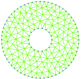
Figure 1: The annulus mesh used for testing in this section.

The boundary conditions used in this test case involve a rotation of the exterior boundary circle by $f$ radians combined with moving the inner boundary by a factor $f$ closer to the outer boundary (where $f=0$ means no motion and $f=1$ means that the inner boundary would coincide with the outer boundary). Values of $f$ tried were $0.1$, $0.3$, $0.6$, and $0.7$. The resulting deformed meshes are illustrated in Fig. 2.

The number of ALS steps to compute these deformed meshes is given in Table 1. The columns of this table are as follows. The first column $f$ is the amount of boundary deformation as described in the previous paragraph. The second column # inv is the number of inverted elements in the deformed mesh prior to application of UBN. The third column UBN–IS is the number of iterations of iterative stiffening required by UBN. The fourth column UBN–NM is the number of iterations of Newton’s method required by UBN. The fifth column UBN-ALS is the number of ALS steps required by UBN (and hence is the sum of the second and third columns).

The remaining columns of the table report on results from the continuation algorithm. The sixth column is the number of major iterations (i.e., updates to the continuation parameter $\tau$) required by the continuation algorithm when constant-size steps are employed. The seventh column is the number of ALS steps required by continuation. The eighth and ninth columns are the same quantities required by the continuation algorithm using the adaptive rule discussed in Section 3 with parameter $\eta=1/3$. The tenth and eleventh columns are the same quantities when $\eta=1.2$. Note that $\eta=1.2$ is a quite aggressive choice of stepsize for continuation, since any value of $\eta>1$ means that updating the boundary could cause an inversion. For this 2D test case, an aggressive choice of $\eta$ did not seem to hinder convergence, but the results for a large value of $\eta$ in 3D described in the next section are less favorable.

For $f=0.8$, neither UBN nor Newton continuation was able to find a solution. UBN’s iterative stiffening did not untangle the mesh after the maximum number of iterations (400) had been reached, and continuation stalled at $\tau=0.93$ when adaptive steps were used and terminated with an inverted element when constant steps were used.

It should be noted that a highly deformed mesh like the solution when $f=0.7$ is probably not physically valid because the finite element discretization is no longer an accurate approximation to the underlying PDE. Nonetheless, we include extreme cases like this because it is interesting to compare the two algorithms in limiting cases. The test results show that UBN is much faster than continuation for both modest and extreme deformations.

Note that for continuation, the outer boundary motion (i.e., the Dirichlet boundary condition) is parametrized in polar coordinates by $\theta$, the rotation angle. Linear parametrization with respect to the rectangular coordinates, $(x,y)$, would work poorly in this case because a linear deformation from the initial position of the outer boundary to the final position would cause the outer boundary to shrink in radius and then expand.

$$\begin{array}[]{cc}\@add@centering\centering\includegraphics[height=113.81102pt]{annulus-def1.eps}&\includegraphics[height=113.81102pt]{annulus-def2.eps}\\ (a)&(b)\\ \includegraphics[height=113.81102pt]{annulus-def3.eps}&\includegraphics[height=113.81102pt]{annulus-def4.eps}\\ (c)&(d)\end{array}$$

Figure 2: Deformed annulus meshes resulting from rotating the exterior boundary circle of the mesh shown in Fig. 1 by $f$ radians and moving the inner boundary circle by a factor $f$ closer to the outer boundary. The deformed meshes are for (a) $f=0.1$, (b) $f=0.3$, (c) $f=0.6$, and (d) $f=0.7$.

Table 1: Results of comparison of UBN to the most efficient version of continuation for the 2D annular domain. See the corresponding text for explanation of the column headers.

$f$	UBN				Contin., tol = $10^{-3}$
					const. steps		$\eta=1/3$		$\eta=1.2$
	# inv	IS	NM	ALS	MajIt	ALS	MajIt	ALS	MajIt	ALS
0.1	0	1	3	4	27	55	28	57	8	18
0.3	36	1	5	6	80	162	87	175	24	50
0.6	59	5	29	34	160	322	265	483	73	148
0.7	64	9	23	32	187	356	414	683	113	228

Comparing the UBN–ALS and Contin–ALS columns of this table indicates that UBN is approximately 9-27 times more efficient than continuation when constant-size steps are used, and is 15 to 30 times more efficient when $\eta=1/3$. (Note that the most efficient results for the UBN and Newton continuation methods are shown in bold face type.) Continuation is $3$ to $4$ times faster when used with the larger value of $\eta$ but is still significantly slower than UBN. Other annulus deformation tests not reported here confirm that UBN is always far more efficient than continuation.

We also wished to check whether the iterative stiffening step in UBN was essential. As evidenced in Column 2 of Table 1, for smaller deformations, the deformed mesh does not always result in inverted elements. However, for larger deformations, the deformation does result in inverted elements. For deformed meshes with inverted elements, the iterative stiffening step is essential to untangling the mesh before using it as a starting point to the line search. For all deformed meshes, it is useful for determining a good starting point.

Similarly, we checked to determine whether the line sea-
rch procedure built into UBN was ever active in order to determine whether it is an essential part of UBN. We found that it was active on about 30%-50% of the iterations for the larger values of deformation.

Table 2: Results of comparison of different versions of continuation for the 2D annular domain. See the corresponding text for explanation of the column headers.

$f$	Contin., tol = $10^{-3}$										Contin., tol = $10^{-5}$
	const. steps		$\eta=1/3$		$\eta=1.2$		$\eta=1/3$ + LS		$\eta=1.2$ + LS		const. steps		$\eta=1/3$		$\eta=1.2$
	MajIt	ALS	MajIt	ALS	MajIt	ALS	MajIt	ALS	MajIt	ALS	MajIt	ALS	MajIt	ALS	MajIt	ALS
0.1	27	55	28	57	8	18	28	57	8	18	27	55	28	57	8	25
0.3	80	162	87	175	24	50	87	175	24	50	80	190	87	179	24	73
0.6	160	322	265	483	73	148	265	483	73	148	160	430	264	545	73	220
0.7	187	356	414	683	113	228	414	683	113	228	187	511	407	832	113	340

Motivated by the robustness issues experienced by the Newton continuation method in 3D, we also wished to investigate the performance of the method when safeguarded steps are taken (by employing the same line search described in Section 5), a tighter convergence tolerance is used, and constant-size steps are employed. The results of our experiments are shown in Table 2. For ease of comparison, the Newton continuation results shown in Table 1 are listed here in columns 2-7. The eighth and ninth columns record the results of adding a line search to the Newton continuation method for the case when $\eta=1/3.$ The tenth and eleventh columns indicate the corresponding information when a line search is used and $\eta=1.2.$ The twelfth and thirteenth columns show the results when constant steps are employed with a convergence tolerance of $10^{-5}.$ The remaining columns specify the results for when the convergence tolerance is $10^{-5}$ and $\eta=1/3$ or $\eta=1.2.$

The results show that the addition of a line search to safeguard the steps of the Newton continuation method is unnecessary whenever the method is able to compute the deformed mesh without experiencing robustness issues. However, the continuation method was able to compute the deformed mesh for $f=0.8$ when a convergence tolerance of $10^{-3}$ and a line search were employed. The use of a tighter convergence tolerance slows down the convergence of the continuation method on these test problems. Taking constant-size steps generally produces convergence more quickly than the use of the conservative adaptive stepping rule but more slowly than the aggressive adaptive stepping rule. However, it should be noted that the use of a convergence tolerance of $10^{-5}$ when taking either constant-size steps or steps computed using the aggressive adaptive step rule were also able to compute a deformed mesh for $f=0.8$. In addition, the faster Newton continuation methods discussed above are up to 4 times faster than the other continuation methods presented here. Thus, the use of a line search and a narrower convergence tolerance should be performed only when the deformation is extremely large, and UBN is not able to compute the deformed mesh.

The use of a line search with a convergence tolerance of $10^{-5}$ was not explored since the use of constant-size steps with the tighter convergence tolerance was the most effective (i.e., the method was even able to compute the deformed mesh for $f=0.9$).

7 3D Experiments

Our experiments in 3D consisted of two tetrahedral meshes called “Hook” and “Foam5,” which were provided to us by P. Knupp pat_mesh . “Hook” is a geometry composed of three main sections: its two end segments are composed of half annuli (in 3D), and its middle section is an irregularly-shaped solid which creates a sharp corner where it joins the bottom section. “Foam5” is a prism whose cross-section is a half-disk with three cavities cut on the top surface; two of the cavities are cylinders and the third is two parallelpipeds arranged like stairs. The sizes of the meshes are as follows: Hook contains 1190 nodes and 4675 tetrahedra, and Foam5 contains 1337 nodes and 4847 tetrahedra. Hook is contained in a bounding box of size $54\times 40\times 95$, while Foam5 is contained in a bounding box of size $11.3\times 5.5\times 6.6$.

In both cases, we applied Dirichlet boundary conditions to two of the boundary surfaces, leaving the rest traction-free. In both cases, the Dirichlet conditions are identically zero on one boundary surface and displace the other surface in a uniform direction. Three magnitudes for the displacement were tested. For Hook, the displacement sizes were 10, 20, and 40, whereas for Foam5 they were 0.5, 2, and 5. Thus, we see that the applied displacements are on the same order as the size of the object, and therefore large deformations will result. Figure 3 shows the deformed and undeformed configurations of Hook for the maximum deformation of 5, while Fig. 4 shows the corresponding illustration of Foam5.

$$\begin{array}[]{cc}\@add@centering\centering\includegraphics[height=142.26378pt]{hookundefln1.eps}&\includegraphics[height=142.26378pt]{hookundefln2.eps}\\ (a)&(b)\\ \includegraphics[height=142.26378pt]{hookdefln1.eps}&\includegraphics[height=142.26378pt]{hookdefln2.eps}\\ (c)&(d)\end{array}$$

Figure 3: The top row line diagrams $(a)$ and $(b)$ show the undeformed Hook body from two different viewpoints. Dirichlet boundary conditions were applied to two of the boundary surfaces to yield deformed meshes. In particular, the asterisks mark the zero-displacement boundary, while the $\times$’s mark fixed displacement. The bottom row diagrams $(c)$ and $(d)$ show Hook after the maximum deformation of 40 is applied.

$$\begin{array}[]{cc}\@add@centering\centering\includegraphics[height=142.26378pt]{foamundefln1.eps}&\includegraphics[height=142.26378pt]{foamundefln2.eps}\\ (a)&(b)\\ \includegraphics[height=142.26378pt]{foamdefln1.eps}&\includegraphics[height=142.26378pt]{foamdefln2.eps}\\ (c)&(d)\end{array}$$

Figure 4: The top row line diagrams $(a)$ and $(b)$ show the undeformed Foam5 body from two different viewpoints. Dirichlet boundary conditions were applied to two of the boundary surfaces to yield deformed meshes. In particular, the asterisks mark the zero-displacement boundary, while the $\times$’s mark fixed displacement. The bottom row diagrams $(c)$ and $(d)$ show Foam5 after the maximum deformation of 5 is applied.

The results of our tests of UBN versus Newton continuation on Hook and Foam5 with a $10^{-3}$ convergence tolerance are given in Table 3. (The relevant column headers are the same as those given for Table 1.) As in the previous section, the unit for measuring running time is ALS steps. For these tests, straight linear parametrization was used for continuation. As before, our results on Hook indicate that UBN is 15 to 50 times faster than continuation when $\eta=1/3$, and 5 to 15 times faster for $\eta=1.2$. In addition, UBN is 15 to 50 times faster than continuation when constant-size steps are taken.

The continuation algorithm terminates when the increment in $\tau$ becomes smaller than the prespecified minimum (0.0005); this happened in two of the tests with Foam5 when $\eta=1/3$ (indicated by ‘—’ in the table). Apparently this is due to an extremely flat tetrahedron which, although it is does not become inverted, causes the heuristic used for adaptively incrementing $\tau$ to take very conservative steps. The continuation algorithm also terminates when inverted elements remain after one major iteration. This happened in one of the tests with Hook when constant-size steps were taken as indicated by ’***’ in the table.

For the Foam5 tests, the continuation algorithm terminated after one major iteration due to the presence of inverted elements for three of the meshes when $\eta=1.2$. This shows that, as expected, the aggressive choice of $\eta$ may be more prone to inverting elements. Similar performance of the continuation algorithm occurred for two of the meshes when constant-size steps were used.

Table 3: Results of comparison of UBN to continuation for 3D domains. See the corresponding text for explanation of the column headers.

mesh	displ.	UBN				Contin., tol = $10^{-3}$
						const. steps		$\eta=1/3$		$\eta=1.2$
		# inv	IS	NM	ALS	MajIt	ALS	MajIt	ALS	MajIt	ALS
Hook	10.0	0	1	5	6	53	107	53	107	15	32
Hook	20.0	0	1	6	7	165	212	105	212	30	61
Hook	40.0	0	1	8	9	***	***	210	421	59	119
Foam5	0.5	18	1	4	5	28	36	28	36	***	***
Foam5	2.0	72	1	5	6	***	***	—	—	***	***
Foam5	5.0	76	1	7	8	***	***	—	—	***	***

Table 4: Results of comparison of different versions of continuation for 3D domains. See the corresponding text for explanation of the column headers.

mesh	displ.	Contin., tol = $10^{-3}$								Contin., tol = $10^{-5}$
		$\eta=1/3$		$\eta=1.2$		$\eta=1/3$ + LS		$\eta=1.2$ + LS		const. steps		$\eta=1/3$		$\eta=1.2$
		MajIt	ALS	MajIt	ALS	MajIt	ALS	MajIt	ALS	MajIt	ALS	MajIt	ALS	Majit	ALS
Hook	10.0	53	107	15	32	53	107	15	32	53	159	53	159	15	46
Hook	20.0	105	212	30	61	105	212	30	61	105	316	105	316	30	91
Hook	40.0	210	421	59	119	210	421	59	119	xxx	xxx	59	177	xxx	xxx
Foam5	0.5	28	36	***	***	28	36	***	***	28	57	8	25	28	57
Foam5	2.0	—	—	***	***	—	—	***	***	110	221	109	219	31	93
Foam5	5.0	—	—	***	***	—	—	***	***	274	549	269	539	75	226

In order to attempt to improve the robustness of the Newton continuation algorithm for the 3D Hook and Foam5 mes-
hes, we also performed experiments which considered the use of a line search to safeguard the steps, the use of constant steps, and the use of a tighter convergence tolerance. The results of our experiments are shown in Table 4. Note that the column headers are identical to those described above for Table 2 (except that the results for taking constant-size steps with a convergence tolerance of $10^{-3}$ has been omitted from the table). The most efficient continuation method results are shown in bold face type.

The results demonstrate that the addition of a line search to the continuation method did not serve to resolve the robustness issues for the method when a convergence tolerance of $10^{-3}$ was employed. However, the use of a tighter convergence tolerance, i.e., $10^{-5}$, (either in combination wi-
th adaptive steps or constant-size steps) served to resolve the robustness problems seen when the looser convergence tolerance was employed. The disadvantage is that the use of a tighter convergence tolerance makes the Newton continuation method much more expensive. In particular, UBN is up to 70 times faster than the slowest Newton continuation method reported here. It should be noted that for one of the Hook test cases, the continuation method terminated after the maximum number of iterations (600) had been performed; this was recorded as an ’xxx’ in the table. The most efficient Newton continuation method is a function of the test problem. For somewhat smaller deformations (as was the case for the Hook mesh), the use of the aggressive adaptive step strategy and the looser convergence tolerance was the most efficient. However, for larger deformations, the use of the aggressive adaptive step strategy with the tighter convergence tolerance was the most efficient. Finally, the UBN method was much more efficient and more robust than the Newton continuation method, in general.

All the preceding tests involved traction free boundaries and prescribed displacements, not all zero, for Dirichlet bou-
ndary nodes. We conclude this section by reporting on experiments with the following boundary conditions. Nonzero tractions were specified on one facet of the Hook mesh, while zero displacements were forced on a different facet. (Tractions were implemented as normally directed point lo-
ads on each node of the facet. For larger loads, this is not a completely realistic approach since realistic forces would change directions under very large deformation, but so-called “follower” loads are beyond the scope of this work.) The remaining boundary nodes were traction-free. Different levels of the traction load were used for different experiment.

These experiments required a modification of our stepping rule for continuation since the rule outlined in Section 3 is intended for nonzero boundary displacements and zero tractions. The modified continuation routine determines a fixed stepsize as follows. First, the same underlying problem is solved using linear elasticity. (It may happen that some elements are inverted in this solution; in this setting, we do not care about element inversion.) From this linear solution, we measure the maximum displacement among nodes. Then the stepsize for continuation is taken to be the quotient of the minimum altitude in the original mesh divided by the maximum displacement in the preliminary solve. The rationale for this rule is so that the amount of deformation that occurs per step of continuation should not exceed the sizes of the elements in an effort to prevent inversions.

This stepsize rule appeared in our experiments to be appropriate in the following sense. Most outer iterations of continuation (i.e., stepping from $\tau_{k}$ to $\tau_{k+1}$) appeared to require 2 to 4 inner Newton iterations. If the usual number required were 1, this would indicate a stepsize which is too small (conservative). On the other hand, if the usual required were much greater than 1, this would indicate that the stepsize is too large for straightforward continuation.

We found that UBN was 2 to 5 times faster than continuation for these test cases. Both algorithms returned a converged solution. In the case of the largest load, the two solutions differed. Both were physically valid; one corresponded to the base of the hook bending toward the hook end in the direction on the inside of the hook, whereas the other corresponded to bending toward the outside of the hook. See remarks on the possibility of multiple solutions in Section 8.

Since all displacement boundary conditions in this example are zero, the possibility of some additional experiments to elucidate features of UBN were carried out. The first experiment on this problem ran the safeguarded Newton method of UBN but omitted the preliminary use of FEMW-
ARP to find a good starting point for the safeguarded Newton method. Instead, the safeguarded Newton method was initialized with the original mesh, which is possible because the prescribed displacement boundary conditions are all zero. We found that the method did not always converge. This shows that even the safeguarded Newton method should be initialized close to the solution else divergence may result. The second additional experiment looked at using unsafeguarded Newton’s method from the initial mesh to find the final configuration. Again, this is possible because of the zero displacement condition. Our experiment indicated that this method did not always converge either. Thus, these experiments provide evidence of the necessity of the iterative stiffening and safeguarded line search.

8 Conclusions

In summary, we developed a robust solution method for solving nonlinear elasticity equations for hyperelastic solids with large boundary deformations. The basic idea is to first untangle the mesh using purely geometric methods and second solve the mechanical model; thus, the algorithm was named UBN (for “untangling before Newton”). The first step of our algorithm is to attempt to untangle the mesh with iterative stiffening. Assuming the mesh is untangled, UBN takes safeguarded Newton steps to solve $(\ref{eq:varform})$.

We tested the robustness of UBN and compared it to the standard Newton continuation algorithm. We demonstrated that UBN is significantly more robust that the Newton continuation algorithm, i.e., it is able to tolerate much larger deformations, in general. For a couple of cases with extremely large deformations, the Newton continuation algorithm with the use of a tight convergence tolerance and very small constant-size steps was the only method which was able to compute the deformed meshes. It is also likely that UBN could compute the deformed meshes if the deformation were broken into smaller deformations (in a similar manner to the small-step FEMWARP algorithm described in ShontzVava ). We also showed that UBN is much faster (i.e., up to 70 times faster) than the Newton continuation algorithm. It could be argued that continuation would be more competitive with UBN if only we had used a different strategy for incrementing $\tau_{k}$. This may be true, but it seems to us that there is no good universal fast method for choosing the $\tau_{k}$. Our experiments indicate, for example, that a more aggressive algorithm for updating $\tau$ is more prone to terminating early due to inverted elements. Even selecting the continuation path seems to be nontrivial (e.g., for the 2D annulus example, it was necessary to parametrize the Dirichlet boundary condition in polar rather than rectangular coordinates). In contrast, the UBN method does not require any such analogous problem-dependent decisions, and the only parameters of the algorithm involve termination criteria.

As described so far, our method applies to finite elements in which the displacement field is piecewise linear over tetrahedra, but UBN could be extended to piecewise quadratic displacements. The challenge with piecewise quad-ratic displacements is that checking for tangling is much more complicated, as $J$ is not constant on the element. In particular, it is a function of both the displacement and the location on the element, which makes it difficult to determine when $J>0$ analytically. There are some separate necessary and sufficient conditions for element inversion in the literature. Let $G$ be the Jacobian of $F$. Then one such necessary condition is that $\det(G)$ has the same sign (strictly positive or strictly negative) at some finite list of test points shephard . In this case, we would test for inversion at the Gauss points used for numerical quadrature; however, it is still possible that folding could occur at the corners. A more complicated sufficient condition for invertibility involving the Bernstein-Bézier form of a polynomial is given in vavasis_bb . Checking that the sufficient condition is met requires running a linear programming algorithm. Salem, Canann, and Saigal have proposed sufficient conditions for quadratic triangles and tetrahedra in salem1 , salem2 , salem3 , and salem4 .

Another issue for UBN is uniqueness. It should be noted that some classes of boundary value problems may admit multiple solutions. A somewhat complicated example of this nonuniqueness occurred in Section 7. A conceptually simpler example is as follows. Consider a long cylinder in which one end is held at zero displacement, the other is rotated by $2\pi$ radians, the long side-surface is traction-free, and there are no body forces. Since the rotated nodes at one end return to their original positions after rotation by $2\pi$ radians, a valid solution to the boundary value problem is all zero displacements. A second valid solution is a twisted configuration of the cylinder.

In the case of continuation, it is possible to select a sequence of nonlinear boundary deformations to force the correct final configuration. This is not possible with UBN, however, at least not without further modification. To distinguish one solution from another requires additional information beyond boundary conditions. Determining what form the additional information ought to take will be studied as future work. We will also determine how UBN should be extended in order to use such additional information.

Future work will also involve extending UBN to the incompressible or nearly incompressible case. In the incompressible case, the requirement that $J=1$ becomes a constraint rather than a term in the energy functional. For this reason, $J$ disappears from the functional. One minimizes $\psi({\bf u})$ subject to the constraint $\mathbf{g}({\bf u})={\bf 0}$, where the latter expresses the $J=1$ constraint for each Gauss point. The functional $\psi({\bf u})$ typically involves the deviatoric strain at Gauss points. A common method for handling a constraint like this is an augmented Lagrangian optimization algorithm NocedalWright . On each iteration of the augmented Lagrangian method, our UBN method is applicable in the same way as in the unconstrained case considered here. In particular, the energy function $\psi({\bf u})$ is usually undefined or nondifferentiable when $J=0$, so Newton’s method is unlikely to work well when $J$ gets close to zero or, even worse, becomes negative. Therefore, the preliminary untangling step and line search described earlier are appropriate for the incompressible case as well.

9 Acknowledgements

The authors wish to thank Patrick Knupp of Sandia National Laboratories for providing us with the 3D test meshes. They benefited from many helpful conversations with Katerina Papoulia of University of Waterloo. They also wish to thank the anonymous referees for their careful reading of the paper and for their helpful suggestions which strengthened it.

References

- (1) G. Holzapfel, Nonlinear Solid Mechanics: A Continuum Approach for Engineering, Wiley, 2000.
- (2) P. Ciarlet and G. Geymonat, Sur les lois de comportement en élasticité non-linéaire compressible, C. R. Acad. Sci. Paris Sér. II, 295: 423-426, 1982.
- (3) M. Mooney, A theory of large elastic deformation, J. Appl. Phys., 11: 582-592, 1940.
- (4) L. Gibson and M. Ashby, Cellular solids. Structure and properties, Cambridge Press, 2nd Edition, 1997.
- (5) F. Weichert and A. Schröder and C. Landes and A. Shamaa and S.K. Awad and L. Walczak and H. Müller and M. Wagner, Computation of a finite element-conformal tetrahedral mesh approximation for simulated soft tissue deformation using a deformable surface model, Med. Biol. Eng. Comput., 48: 597-610, 2010.
- (6) T. Belytschko and W. Liu and B. Moran, Nonlinear Finite Elements for Continua and Structures, Wiley, 2000.
- (7) T. J. R. Hughes, The Finite Element Method: Linear Static and Dynamic Finite Element Analysis, Dover Publishers, 2000.
- (8) P. Keast, Moderate-degree tetrahedral quadrature formulas, Comput. Methods Appl. Mech. Eng., 55: 339-48, 1986.
- (9) S. Shontz and S. Vavasis, Analysis of and workarounds for element reversal for a finite element-based algorithm for warping triangular and tetrahedral meshes, BIT, Numerical Mathematics, 50(4): 863-884, 2010.
- (10) S. Wright, Primal-Dual Interior-Point Methods, Society for Industrial and Applied Mathematics, 1997.
- (11) K. Stein and T. Tezduyar and R. Benney, Moving mesh techniques for fluid-structure interactions with large displacements, Journal of Applied Mechanics (ASME), 70: 58-63, 2003.
- (12) S. M. Shontz, Numerical Methods for Problems with Moving Meshes, Ph.D. Thesis, Cornell University, 2005.
- (13) L. Freitag and P. Plassmann, Local optimization-based simplicial mesh untangling and improvement, Int. J. Numer. Methods Eng., 49: 109-125, 2000.
- (14) G. H. Golub and C. F. Van Loan, Matrix Computations, Johns Hopkins University Press, 3rd Edition, 1996.
- (15) J. E. Dennis, Jr. and R. B. Schnabel, Numerical Methods for Unconstrained Optimization and Nonlinear Equations, Society for Industrial and Applied Mathematics, 1996.
- (16) J. Shewchuk, Triangle: Engineering a 2D quality mesh generator and Delaunay triangulator, in Proceedings of the First Workshop on Applied Computational Geometry, Association for Computing Machinery, pp. 124-133, 1996.
- (17) P. Knupp, Sandia National Laboratories, Personal communication, 2003.
- (18) M. Shephard and S. Dey and M. Georges, Automatic meshing of curved three-dimensional domains: Curving finite elements and curvature-based mesh control, in I. Babuska and J. Flaherty and J. Hopcroft and W. Henshaw and J. Oliger and T. Tezduyar (Eds.), Modeling, Mesh Generation, and Adaptive Numerical Methods for Partial Differential Equations, Springer-Verlag, 1995.
- (19) S. Vavasis, A Bernstein-Bézier sufficient condition for invertibility of polynomial mappings, Archived by arxiv.org, cs.NA/0308021, 2003.
- (20) A. Salem and S. Canann and S. Saigal, Robust quality metric for quadratic triangular 2D finite elements, Trends in Unstructured Mesh Generation, 220: 73-80, 1997.
- (21) A. Salem and S. Canann and S. Saigal, Mid-node admissible spaces for quadratic triangular 2D arbitrarily curved finite elements, Int. J. Numer. Methods Eng., 50: 253-272, 2001.
- (22) A. Salem and S. Canann and S. Saigal, Mid-node admissible spaces for quadratic triangular 2D finite elements with one edge curved, Int. J. Numer. Methods Eng., 50: 181-197, 2001.
- (23) A. Salem and S. Saigal and S. Canann, Mid-node admissible space for 3D quadratic tetrahedral finite elements, Eng. Comput., 17: 39-54, 2001.
- (24) J. Nocedal and S. J. Wright, Numerical Optimization, Springer-Verlag, 2nd Edition, 2006.