The Haar Wavelet Transform of a Dendrogram

Abstract

We describe a new wavelet transform, for use on hierarchies or binary rooted trees. The theoretical framework of this approach to data analysis is described. Case studies are used to further exemplify this approach. A first set of application studies deals with data array smoothing, or filtering. A second set of application studies relates to hierarchical tree condensation. Finally, a third study explores the wavelet decomposition, and the reproducibility of data sets such as text, including a new perspective on the generation or computability of such data objects.

Keywords: multivariate data analysis, hierarchical clustering, data summarization, data approximation, compression, wavelet transform, computability.

1 Introduction

In this paper, the new data analysis approach to be described can be understood as a transform which maps a hierarchical clustering into a transformed set of data; and this transform is invertible, meaning that the original data can be exactly reconstructed. Such transforms are very often used in data analysis and signal processing because processing of the data may be facilitated by carrying out such processing in transform space, followed by reconstruction of the data in some “good approximation” sense.

Consider data smoothing as a case in point of such processing. Smoothing of data is important for exploratory visualization, for data understanding and interpretation, and as an aid in model fitting (e.g., in time series analysis or more generally in regression modeling). The wavelet transform is often used for signal (and image) smoothing in view of its “energy compaction” properties, i.e., large values tend to become larger, and small values smaller, when the wavelet transform is applied. Thus a very effective approach to signal smoothing is to selectively modify wavelet coefficients (for example, put small wavelet coefficients to zero) before reconstructing an approximate version of the data. See Härdle (2000), Starck and Murtagh (2006).

The wavelet transform, developed for signal and image processing, has been extended for use on relational data tables and multidimensional data sets (Vitter and Wang, 1999; Joe, Whang and Kim, 2001) for data summarization (micro-aggregation) with the goal of anonymization (or statistical disclosure limitation) and macrodata generation; and data summarization with the goal of computational efficiency, especially in query optimization. A survey of data mining applications (including applications to image and signal content-based information retrieval) can be found in Tao Li, Qi Li, Shenghuo Zhu and Ogihara (2002).

A hierarchical representation is used by us, as a first phase of the processing, (i) in order to cater for the lack of any inherent row/column order in the given data table and to get around this obstacle to freely using a wavelet transform; and (ii) to take into account structure and interrelationships in the data. For the latter, a hierarchical clustering furnishes an embedded set of clusters, and obviates any need for a priori fixing of number of clusters. Once this is done, the hierarchy is wavelet transformed. The approach is a natural and integral one.

Our innovation is to apply the Haar wavelet transform to a binary rooted tree (viz., the clustering hierarchy) in terms of the following algorithm: recursively carry out pairwise averaging and differencing at the sequence of levels in the tree.

A hierarchy may be constructed through use of any constructive, hierarchical clustering algorithm (Benzécri, 1979; Johnson, 1967; Murtagh, 1985). In this work we will assume that some agglomerative criterion is satisfactory from the perspective of the type of data, and the nature of the data analysis or processing. In a wide range of practical scenarios, the minimum variance (or Ward) agglomerative criterion can be strongly recommended due to its data summarizing properties (Murtagh, 1985).

The remainder of this article is organized as follows. Sections 2 and 3 present important background context. Section 4 presents our new wavelet transform. In section 5, illustrative case studies are used to further discuss the new approach. Section 6 deals with the application to data array smoothing, or filtering. Section 7 deals with the application to hierarchical tree condensation. Section 8 explores the wavelet decomposition, and linkages with reproducibility or recreation of data sets such as text.

2 Wavelets on Local Fields

Wavelet transform analysis is the determining of a “useful” basis for $L^{2}(\mathbb{R}^{m})$ which is induced from a discrete subgroup of $\mathbb{R}^{m}$, and uses translations on this subgroup, and dilations of the basis functions.

Classically (Frazier, 1999; Debnath and Mikusiński, 1999; Strang and Nguyen, 1996) the wavelet transform avails of a wavelet function $\psi(x)\in L^{2}(\mathbb{R})$, where the latter is the space of all square integrable functions on the reals. Wavelet transforms are bases on $L^{2}(\mathbb{R}^{m})$, and the discrete lattice subgroup $\mathbb{Z}^{m}$ ($m$-dimensional integers) is used to allow discrete groups of dilated translation operators to be induced on $\mathbb{R}^{m}$. Discrete lattice subgroups are typical of 2D images (where the lattice is a pixelated grid) or 3D images (where the lattice is a voxelated grid) or spectra or time series (the lattice is the set of time steps, or wavelength steps).

Sometimes it is appropriate to consider the construction of wavelet bases on $L^{2}(G)$ where $G$ is some group other than $\mathbb{R}$. In Foote, Mirchandani, Rockmore, Healy and Olson (2000a, 2000b; see also Foote, 2005) this is done for the group defined by a quadtree, in turn derived from a 2D image. To consider the wavelet transform approach not in a Hilbert space but rather in locally-defined and discrete spaces we have to change the specification of a wavelet function in $L^{2}(\mathbb{R})$ and instead use $L^{2}(G)$.

Benedetto (2004) and Benedetto and Benedetto (2004) considered in detail the group $G$ as a locally compact abelian group. Analogous to the integer grid, $\mathbb{Z}^{m}$, a compact subgroup is used to allow a discrete group of operators to be defined on $L^{2}(G)$. The property of locally compact (essentially: finite and free of edges) abelian (viz., commutative) groups that is most important is the existence of the Haar measure. The Haar measure allows integration, and definition of a topology on the algebraic structure of the group.

Among the cases of wavelet bases constructed via a sub-structure are the following (Benedetto, 2004).

• Wavelet basis on $L^{2}(\mathbb{R}^{m})$ using translation operators defined on the discrete lattice, $\mathbb{Z}^{m}$. This is the situation that holds for image processing, signal processing, most time series analysis (i.e., with equal length time steps), spectral signal processing, and so on. As pointed out by Foote (2005), this framework allows the multiresolution analysis in $L^{2}(\mathbb{R}^{m})$ to be generalized to $L^{p}(\mathbb{R}^{m})$ for Minkowski metric $L^{p}$ other than Euclidean $L^{2}$.

• Wavelet basis on $L^{2}(\mathbb{Q}_{p})$, where $\mathbb{Q}_{p}$ is the p-adic field, using a discrete set of translation operators. This case has been studied by Kozyrev, 2002, 2004; Altaisky, 2004, 2005. See also the interesting overview of Khrennikov and Kozyrev (2006).

• Finally the central theme of Benedetto (2004) is a wavelet basis on $L^{2}(G)$ where $G$ is a locally compact abelian group, using translation operators defined on a compact open subgroup (or operators that can be used as such on a compact open subgroup); and with definition of an expansive automorphism replacing the traditional use of dilation.

In Murtagh (2006) the latter theme is explored: a p-adic representation of a dendrogram is used, and an expansive operator is defined, which, when applied to a level of a dendrogram enables movement up a level.

In our case we are looking for a new basis for $L^{2}(G)$ where $G$ is the set of all equivalent representations of a hierarchy, $H$, on $n$ terminals. Denoting the level index of $H$ as $\nu$ (so $\nu:H\longrightarrow\mathbb{R}^{+}$, where $\mathbb{R}^{+}$ are the positive reals), and $\nu=0$ is the level index corresponding to the fine partition of singletons, then this hierarchy will also be denoted as $H_{\nu=0}$. Let $I$ be the set of observations. Let the succession of clusters associated with nodes in $H$ be denoted $Q=\{q_{1},q_{2},\dots,q_{n-1}\}$. We have $n-1$ non-singleton nodes in $H$, associated with the clusters, $q$. At each node we can interchange left and right subnodes. Hence we have $2^{n-1}$ equivalent representations of $H$, or, again, members in the group, $G$, that we are considering.

So we have the group of equivalent dendrogram representations on $H_{\nu=0}$. We have a series of subgroups, $H_{{\nu}_{k}}\supset H_{{\nu}_{(k+1)}}$, for $0\leq k<n-1$. Symmetries (in the group sense) are given by permutations at each level, $\nu$, of hierarchy $H$. Collecting these furnishes a group of symmetries on the terminal set of any given (non-terminal) node in $H$.

We want to process dendrograms, and we want our processing to be invariant relative to any equivalent representation of a given dendrogram.

Denote the permutation at level $\nu$ by $P_{\nu}$. Then the automorphism group is given by:

$$G=P_{n-1}\ \mathrm{wr}\ P_{n-2}\ \mathrm{wr}\ \dots\ \mathrm{wr}\ P_{2}\ \mathrm{wr}\ P_{1}$$

where wr denotes the wreath product.

Foote et al. (2000a, 200b) and Foote (2005) consider the wreath product group of a tree representation of data, including the quadtree which is a tree representation of an image. Just as for us here, the offspring nodes of any given node in such a tree can be “rotated” ad lib. Group action amounts to cyclic shifts or adjacency-preserving permutations of the offspring nodes. The group in this case is referred to as the wreath product group.

We will introduce and study a wavelet transform on $L(G)$ where $G$ is the wreath product group based on the hierarchy or rooted binary tree, $H$.

3 Hierarchy, Binary Tree, and Ultrametric Topology

A short set of definitions follow, showing how a hierarchy is taken in the form of a binary tree, and the particular form of binary tree used here is often termed a dendrogram. By small abuse of terminology, we will use $H$ to denote this hierarchy, and the ultrametric topology that it represents.

A hierarchy, $H$, is defined as a binary, rooted, unlabeled, node-ranked tree, also termed a dendrogram (Benzécri, 1979; Johnson, 1967; Lerman, 1981; Murtagh, 1985). A hierarchy defines a set of embedded subsets of a given set, $I$. However these subsets are totally ordered by an index function $\nu$, which is a stronger condition than the partial order required by the subset relation. A bijection exists between a hierarchy and an ultrametric space.

Let us show these equivalences between embedded subsets, hierarchy, and binary tree, through the constructive approach of inducing $H$ on a set $I$.

Hierarchical agglomeration on $n$ observation vectors, $i\in I$, involves a series of $1,2,\dots,n-1$ pairwise agglomerations of observations or clusters, with the following properties. A hierarchy $H=\{q|q\in 2^{I}\}$ such that (i) $I\in H$, (ii) $i\in H\ \forall i$, and (iii) for each $q\in H,q^{\prime}\in H:q\cap q^{\prime}\neq\emptyset\Longrightarrow q\subset q^{\prime}\mbox{ or }q^{\prime}\subset q$. Here we have denoted the power set of set $I$ by $2^{I}$. An indexed hierarchy is the pair $(H,\nu)$ where the positive function defined on $H$, i.e., $\nu:H\rightarrow\mathbb{R}^{+}$, satisfies: $\nu(i)=0$ if $i\in H$ is a singleton; and (ii) $q\subset q^{\prime}\Longrightarrow\nu(q)<\nu(q^{\prime})$. Here we have denoted the positive reals, including 0, by $\mathbb{R}^{+}$. Function $\nu$ is the agglomeration level. Take $q\subset q^{\prime}$, let $q\subset q^{\prime\prime}$ and $q^{\prime}\subset q^{\prime\prime}$, and let $q^{\prime\prime}$ be the lowest level cluster for which this is true. Then if we define $D(q,q^{\prime})=\nu(q^{\prime\prime})$, $D$ is an ultrametric. In practice, we start with a Euclidean or other dissimilarity, use some criterion such as minimizing the change in variance resulting from the agglomerations, and then define $\nu(q)$ as the dissimilarity associated with the agglomeration carried out.

4 The Hierarchic Haar Wavelet Transform Algorithm: Description

Linkages between the classical wavelet transform, as used in signal processing, and multivariate data analysis, were investigated in Murtagh (1998). The wavelet transform to be described now is fundamentally different, and works on a hierarchy.

The traditional Haar wavelet transform can be simply described in terms of the following algorithm: recursively carry out averaging and differencing of adjacent pairs of data values (pixels, voxels, time steps, etc.) at a sequence of geometrically (factor 2) increasing resolution levels. As mentioned in the Introduction, our innovation is to apply the Haar wavelet transform to the clustering hierarchy, and this algorithm is the recursive carrying out of pairwise averaging and differencing at the sequence of levels in the hierarchical tree.

4.1 Short Description of the Algorithm

A dendrogram on $n$ terminal nodes, associated with observation vectors, has $n-1$ non-terminal nodes. We proceed through each of these non-terminal nodes in turn, starting at the node corresponding to the sequentially first agglomeration, continuing to the node corresponding to the sequentially second agglomeration, and so on, until we finally reach the root node. At each node, we define a vector as the (unweighted) average of the vectors of its two child nodes. So the vector associated with the very first non-terminal node will be the (unweighted) average of the vectors comprising this node’s two (terminal) child nodes.

For subsequent non-terminal nodes, their child nodes may be terminal or non-terminal. In all cases, this procedure is well-defined. We continue the procedure until we have processed all $n-1$ non-terminal nodes.

We now have an increasingly smooth vector corresponding to each node in the dendrogram, or hierarchy, $H$. We term this vector at each node the smooth signal or just smooth at each node.

The detail signal, or detail, at each node is defined as the vector difference between the vector at a (non-terminal) node, and the vector at its (terminal or non-terminal) child node. By consistently labeling left and right child subnodes, by construction the left child subnode will have a detail vector which is just the negative of the detail vector of the right subnode. Hence, with consistency of left and right labeling, we just need to store one of these detail vectors.

Because of the way that the detail signal has been defined, and given the smooth signal associated with the root node (the node with sequence number $n-1$), we can easily see the following: to reconstruct the original data, used to set this algorithm underway, we need just the set of all detail signals, and the final, or root node, smooth signal.

4.2 Definition of Smooth Signals and Detail Signals

Consider any hierarchical clustering, $H$, represented as a binary rooted tree. For each cluster associated with a non-terminal node, $q^{\prime\prime}$, with offspring (terminal or non-terminal) nodes $q$ and $q^{\prime}$, we define $s(q^{\prime\prime})$ through application of the low-pass filter $\left(\begin{array}[]{r}\frac{1}{2}\\ \frac{1}{2}\end{array}\right)$ which can be implemented as a scalar product:

$$s(q^{\prime\prime})=\frac{1}{2}\left(s(q)+s(q^{\prime})\right)=\left(\begin{array}[]{r}0.5\\ 0.5\end{array}\right)^{t}\left(\begin{array}[]{c}s(q)\\ s(q^{\prime})\end{array}\right)$$ (1)

The application of the low-pass filter is carried out in order of increasing node number (i.e., from the smallest non-terminal node, through to the root node). For a terminal node, $i$, allowing us to notationally say that $q=i$ or that $q^{\prime}=i$, the signal smooth $s(i)$ is just the given vector, and this aspect is addressed further below, in subsection 4.3.

Next for each cluster $q^{\prime\prime}$ with offspring nodes $q$ and $q^{\prime}$, we define detail coefficients $d(q^{\prime\prime})$ through application of the band-pass filter $\left(\begin{array}[]{r}\frac{1}{2}\\ -\frac{1}{2}\end{array}\right)$:

$$d(q^{\prime\prime})=\frac{1}{2}(s(q)-s(q^{\prime}))=\left(\begin{array}[]{r}0.5\\ -0.5\end{array}\right)^{t}\left(\begin{array}[]{c}s(q)\\ s(q^{\prime})\end{array}\right)$$ (2)

Again, increasing order of node number is used for application of this filter.

The scheme followed is illustrated in Figure 1, which shows the hierarchy (constructed by the median agglomerative method, although this plays no role here), using for display convenience just the first 8 observation vectors in Fisher’s iris data (Fisher, 1936).

Figure 1: Dendrogram on 8 terminal nodes constructed from first 8 values of Fisher iris data. (Median agglomerative method used in this case.) Detail or wavelet coefficients are denoted by $d$, and data smooths are denoted by $s$. The observation vectors are denoted by $x$ and are associated with the terminal nodes. Each signal smooth, $s$, is a vector. The (positive or negative) detail signals, $d$, are also vectors. All these vectors are of the same dimensionality.

We call our algorithm a Haar wavelet transform because, traditionally, this wavelet transform is defined by a similar set of averages and differences. The former, low-pass filter, is used to set the center of the two clusters being agglomerated; and the latter, band-pass filter, is used to set the deviation or discrepancy of these two clusters from the center.

4.3 The Input Data

We now return to the issue of how we start this scheme, i.e. how we define $s(i)$, or the “smooth” of a terminal node, representing a singleton cluster.

Let us consider two cases:

1. $s(i)$ is a vector in $\mathbb{R}^{m}$, and the $i$th row of a data table.

2. $s(i)$ is an $n$-dimensional indicator vector. So the third, in sequence, out of a population of $n=8$ observations has indicator vector $\{00100000\}$. We can of course take a data table of all indicator vectors: it is clear that the data table is symmetric, and is none other than the identity matrix.

Our hierarchical Haar wavelet transform can easily handle either case, depending on the input data table used.

While we have considered two cases of input data, we may note the following. Having the clustering hierarchy built on the same input data as used for the hierarchical Haar transform is reasonable when compression of the input data is our target. However, if the hierarchical Haar transform is used for data approximation, cf. section 8 below, then we are at liberty to use different data for the hierarchical clustering and for the Haar transform. The hierarchy is built from a set of observation vectors in $\mathbb{R}^{m}$. Then it is used in the Haar wavelet transform as a structure on another set of vectors in $\mathbb{R}^{m^{\prime}}$ (with $m^{\prime}$ not necessarily equal to $m$). We will not pursue this line of investigation further here.

4.4 The Inverse Transform

Constructing the hierarchical Haar wavelet transformed data is referred to as the forward transform. Reconstructing the input data is referred to as the inverse transform.

The inverse transform allows exact reconstruction of the input data. We begin with $s_{n-1}$. If this root node has subnodes $q$ and $q^{\prime}$, we use $d(q)$ and $d(q^{\prime})$ to form $s(q)$ and $s(q^{\prime})$.

We continue, step by step, until we have reconstructed all vectors associated with terminal nodes.

4.5 Matrix Representation

Let our input data be a set of $n$ points in $\mathbb{R}^{m}$ given in the form of matrix $X$. We have:

$$X=CD+S_{n-1}$$ (3)

where $D$ is the matrix collecting all wavelet projections or detail coefficients, $d$. The dimensions of $D$ are $(n-1)\times m$. The dimensions of $C$ are: $n\times(n-1)$. $C$ is a characteristic matrix representing the dendrogram. Murtagh (2006) provides an introduction to $C$, which will be summarized here. In Figure 2, the 0 or 1 coding works well when we also take account of the existence of the node at that particular level. Other forms of coding can be used, and Murtagh (2006) uses a ternary code, viz., $+1$ and $-1$ for left and right branches (replacing 0 and 1 in Figure 2, respectively), and 0 to indicate non-existence of a node at that particular level.

Matrix $C$, describing the branching codes $+1$ and $-1$, and an absent or non-existent branching given by $0$, uses a set of values $c_{ij}$ where $i\in I$, the indices of the object set; and $j\in\{1,2,\dots,n-1\}$, the indices of the dendrogram levels or nodes ordered increasingly. For Figure 2 we have:

$$C=\{c_{ij}\}=\left(\begin{array}[]{rrrrrrr}1&1&0&0&1&0&1\\ -1&1&0&0&1&0&1\\ 0&-1&0&0&1&0&1\\ 0&0&1&1&-1&0&1\\ 0&0&-1&1&-1&0&1\\ 0&0&0&-1&-1&0&1\\ 0&0&0&0&0&1&-1\\ 0&0&0&0&0&-1&-1\end{array}\right)$$ (4)

For given level $j$, $\forall i$, the absolute values $|c_{ij}|$ give the membership function either by node, $j$, which is therefore read off columnwise; or by object index, $i$ which is therefore read off rowwise.

If $s_{n-1}$ is the final data smooth, in the limit for very large $n$ a constant-valued $m$-component vector, then let $S_{n-1}$ be the $n\times m$ matrix with $s_{n-1}$ repeated on each of the $n$ rows.

Consider the $j$th coordinate of the $m$-dimensional observation vector corresponding to $i$. For any $d(q_{j})$ we have: $\sum_{k}d(q_{j})_{k}=0$, i.e. the detail coefficient vectors are each of zero mean.

In the case where out input data consists of $n$-dimensional indicator vectors (i.e., the $i$th vector contains 0-values except for location $i$ which has a 1-value), then our initial data matrix $X$ is none other than the $n\times n$ dimensional identity matrix. We will write $X_{\mbox{ind}}$ for this identity matrix.

The wavelet transform in this case is: $X_{\mbox{ind}}=CD+S_{n-1}$.

$X_{\mbox{ind}}$ is of dimensions $n\times n$.

$C$, exactly as before, is a characteristic matrix representing the dendrogram used, and is of dimensions $n\times(n-1)$.

$D$, of necessity different in values from case 1, is of dimensions $(n-1)\times n$.

$S_{n-1}$, of necessity different in values from case 1, is of dimensions $n\times n$.

4.6 Computational Complexity Properties

The computational complexity of our algorithms are as follows. The hierarchical clustering is $O(n^{2})$. The forward hierarchical Haar wavelet transform is $O(n)$. Finally, the inverse wavelet transform is $O(n^{2})$. On Macintosh G4 or G5 machines, all phases of the processing took typically 4–5 minutes for an array of dimensions $12000\times 400$.

An exemplary pipeline of C and R code used in this work is available at the following address: http://astro.u-strasbg.fr/$\sim$fmurtagh/mda-sw

5 Hierarchical Haar Wavelet Transform: Case Studies

In a practical way, using small data sets, we will describe our new hierarchical Haar wavelet transform in this section.

Let us begin with the indicator vectors case. Thus in Figure 2, $x_{1}=\{100000000\}$, and $q_{1}=\{11000000\}$. Note that this is our definition of $x_{1}$ etc. (and is not read off the tree), and from the definition of $x_{1}$ and $x_{2}$ we have defined $q_{1}$. This form of coding was used by Nabben and Varga (1994).

Now we use equations 1 and 2.

Figure 2: Labeled, ranked dendrogram on 8 terminal nodes. Branches labeled 0 and 1.

5.1 Case Study 1

In Figure 2, we have:

$s(q_{1})=\frac{1}{2}(x_{1}+x_{2})=(\frac{1}{2}\ \frac{1}{2}\ 0\ 0\ 0\ 0\ 0\ 0)$

Also: $s(q_{1})=\frac{1}{2}q_{1}$

$s(q_{2})=\frac{1}{2}(s(q_{1})+x_{3})=(\frac{1}{4}\ \frac{1}{4}\ \frac{1}{2}\ 0\ 0\ 0\ 0\ 0)$

Also: $s(q_{2})=\frac{1}{2}(\frac{1}{2}q_{1}+x_{3})=\frac{1}{4}q_{1}+\frac{1}{2}x_{3}$

$s(q_{3})=\frac{1}{2}(x_{4}+x_{5})=(0\ 0\ 0\ \frac{1}{2}\ \frac{1}{2}\ 0\ 0\ 0)$

Also: $s(q_{3})=\frac{1}{2}q_{3}$

$s(q_{4})=\frac{1}{2}(s(q_{3})+x_{6})=(0\ 0\ 0\ \frac{1}{4}\ \frac{1}{4}\ \frac{1}{2}\ 0\ 0)$

$s(q_{5})=\frac{1}{2}(s(q_{2})+s(q_{4}))=(\frac{1}{8}\ \frac{1}{8}\ \frac{1}{4}\ \frac{1}{8}\ \frac{1}{8}\frac{1}{4}\ 0\ 0)$

$s(q_{6})=\frac{1}{2}(x_{7}+x_{8})=(0\ 0\ 0\ 0\ 0\ 0\ \frac{1}{2}\ \frac{1}{2})$

$s(q_{7})=\frac{1}{2}(q_{5}+q_{6})=(\frac{1}{16}\ \frac{1}{16}\ \frac{1}{8}\ \frac{1}{16}\ \frac{1}{16}\ \frac{1}{8}\ \frac{1}{4}\ \frac{1}{4})$

Next we turn attention to the detail coefficients.

$d(q_{1})=\frac{1}{2}(x_{1}-x_{2})=(\frac{1}{2}\ -\frac{1}{2}\ 0\ 0\ 0\ 0\ 0\ 0)$

Alternatively, for $q^{\prime\prime}=q\cup q^{\prime}$, the detail coefficients are defined as: $d(q^{\prime\prime})=s(q^{\prime\prime})-s(q^{\prime})=-(s(q^{\prime\prime})-s(q))$.

Thus $d(q_{1})=s(q_{1})-x_{2}=(\frac{1}{2}\ \frac{1}{2}\ 0\ 0\ 0\ 0\ 0\ 0)-(0\ 1\ 0\ 0\ 0\ 0\ 0\ 0)=(\frac{1}{2}\ -\frac{1}{2}\ 0\ 0\ 0\ 0\ 0\ 0)$

For any $d(q_{j})$ we have: $\sum_{k}d(q_{j})_{k}=0$, i.e. the detail coefficient vectors are each of zero mean.

Let us redo in vector and matrix terms this description of the hierarchical Haar wavelet transform algorithm.

We take our initial or input data as follows.

$$\left(\begin{array}[]{c}x_{1}\\ x_{2}\\ x_{3}\\ x_{4}\\ x_{5}\\ x_{6}\\ x_{7}\\ x_{8}\end{array}\right)=\left(\begin{array}[]{cccccccc}1&0&0&0&0&0&0&0\\ 0&1&0&0&0&0&0&0\\ 0&0&1&0&0&0&0&0\\ 0&0&0&1&0&0&0&0\\ 0&0&0&0&1&0&0&0\\ 0&0&0&0&0&1&0&0\\ 0&0&0&0&0&0&1&0\\ 0&0&0&0&0&0&0&1\end{array}\right)$$ (5)

The hierarchical Haar wavelet transform of this input data is then as follows.

$$\left(\begin{array}[]{c}d(q_{1})\\ d(q_{2})\\ d(q_{3})\\ d(q_{4})\\ d(q_{5})\\ d(q_{6})\\ d(q_{7})\\ s_{7}\end{array}\right)=$$

$$\left(\begin{array}[]{rrrrrrrr}\frac{1}{2}&-\frac{1}{2}&0&0&0&0&0&0\\ \frac{1}{4}&\frac{1}{4}&-\frac{1}{2}&0&0&0&0&0\\ 0&0&0&\frac{1}{2}&-\frac{1}{2}&0&0&0\\ 0&0&0&\frac{1}{4}&\frac{1}{4}&-\frac{1}{2}&0&0\\ \frac{1}{8}&\frac{1}{8}&\frac{1}{4}&-\frac{1}{8}&-\frac{1}{8}&-\frac{1}{4}&0&0\\ 0&0&0&0&0&0&\frac{1}{2}&-\frac{1}{2}\\ \frac{1}{16}&\frac{1}{16}&\frac{1}{8}&\frac{1}{16}&\frac{1}{16}&\frac{1}{8}&-\frac{1}{4}&-\frac{1}{4}\\ \frac{1}{16}&\frac{1}{16}&\frac{1}{8}&\frac{1}{16}&\frac{1}{16}&\frac{1}{8}&\frac{1}{4}&\frac{1}{4}\end{array}\right)$$ (6)

As already noted in this subsection, the succession of $n-1$ wavelet coefficient vectors are of zero mean. Therefore, due to the input data used (relation (5)), each row of the right hand matrix in equation 6 is of zero mean.

Note that this transform is a function of the hierarchy, $H$. Here we are using the hierarchy of Figure 2. $H$ is needed to define the structure of the right hand matrix in equation 6. (This is closely related to the discussion in subsection 4.5. Further discussion can be found in Murtagh, 2006).

5.2 Case Study 2

In Tables 1 and 2 we directly transform a small data set consisting of the first 8 observations in Fisher’s iris data.

Note that in Table 2 it is entirely appropriate that at more smooth levels (i.e., as we proceed through levels d1, d2, $\dots$, d6, d7) the values become more “fractionated” (i.e., there are more values after the decimal point).

The minimum variance agglomeration criterion, with Euclidean distance, is used to induce the hierarchy on the given data. Each detail signal is of dimension $m=4$ where $m$ is the dimensionality of the given data. The smooth signal is of dimensionality $m$ also. The number of detail or wavelet signal levels is given by the number of levels in the labeled, ranked hierarchy, i.e. $n-1$.

	Sepal.L	Sepal.W	Petal.L	Petal.W
1	5.1	3.5	1.4	0.2
2	4.9	3.0	1.4	0.2
3	4.7	3.2	1.3	0.2
4	4.6	3.1	1.5	0.2
5	5.0	3.6	1.4	0.2
6	5.4	3.9	1.7	0.4
7	4.6	3.4	1.4	0.3
8	5.0	3.4	1.5	0.2

Table 1: First 8 observations of Fisher’s iris data. L and W refer to length and width.

	s7	d7	d6	d5	d4	d3	d2	d1
Sepal.L	5.146875	0.253125	0.13125	0.1375	$-0.025$	0.05	$-0.025$	0.05
Sepal.W	3.603125	0.296875	0.16875	$-0.1375$	0.125	0.05	$-0.075$	$-0.05$
Petal.L	1.562500	0.137500	0.02500	0.0000	0.000	$-0.10$	0.050	0.00
Petal.W	0.306250	0.093750	$-0.01250$	$-0.0250$	0.050	0.00	0.000	0.00

Table 2: The hierarchical Haar wavelet transform resulting from use of the first 8 observations of Fisher’s iris data shown in Table 1. Wavelet coefficient levels are denoted d1 through d7, and the continuum or smooth component is denoted s7.

5.3 Traditional versus Hierarchical Haar Wavelet Transforms

Consider a set of 8 input data objects, each of which is scalar:
$(64,48,16,32,56,56,48,24)$. A traditional Haar wavelet transform of this data can be quickly done, and gives: $(43,-3,16,10,8,-8,0,12)$. Here, the first value is the final smooth, and the remaining values are the wavelet coefficients read off by a traversal from final smooth towards the input data values. Showing the output in the same way, the hierarchical Haar wavelet transform of the same data gives: $(40,14,6,-6,-4,4,0,0)$.

A little reflection shows that the greater number of zeros in the hierarchical Haar wavelet transform is no accident. In fact, with the following conditions: 10 different digits in the input data; processing of an $n$-length string of digits; equal frequencies of digits (if necessary, supported by a supposition of large $n$); and use of an unweighted average agglomerative criterion; we have the following.

The hierarchy begins with nodes that agglomerate identical values, $n/2$ of them; followed by agglomeration of the next round of $n/4$ values; followed by $n/8$ agglomerations of identical values; etc. So we have, in all, $n/2+n/4+n/8+\dots+n/2^{n-1}$ identical value agglomerations. All of these will give rise to 0-valued detail coefficients. For suitable $n$, all save the very last round of 10 agglomerations will give rise to non-0 valued detail coefficients.

This remarkable result points to the powerful data compression potential of the hierarchical Haar wavelet transform. We must note though that this rests on the dendrogram, and the computational requirements of the latter are not in any way bypassed.

6 Hierarchical Wavelet Smoothing and Filtering

Previous work on wavelet transforms of data tables includes Chakrabarti, Garofalakis, Rastogi and Shim (2001) and Vitter and Wang (1999). There are problems, however, in directly applying a wavelet transform to a data table. Essentially, a relational table (to use database terminology; or matrix) is treated in the same way as a 2-dimensional pixelated image, although the former case is invariant under row and column permutation, whereas the latter case is not (Murtagh, Starck and Berry, 2000). Therefore there are immediate problems related to non-uniqueness, and data order dependence. What if, however, one organizes the data such that adjacency has a meaning? This implies that similarly-valued objects, and/or similarly-valued features, are close together. This is what we do, using any hierarchical clustering algorithm.

From a given input data array, the hierarchical wavalet transform creates an output data array with the property of forcing similar values to be close together. This transform is fully reversible. The proximity of similar values, however, is with respect to the hierarchical tree which was used in the forward transform, and of course comes into play also in the inverse transform. Because similar values are close together, the compressibility of the transformed data is enhanced. Separately, setting small values in the transformed data to zero allows for data smoothing or data “filtering”.

6.1 The Smoothing Algorithm

We use the following generic data analysis processing path, which is applicable to any input tabular data array of numerical values. We assume only that there are no missing values in the data array.

1. Given a dissimilarity, induce a hierarchy on the set of observations. (We generally use the Euclidean distance, and the minimum variance agglomerative hierarchical clustering criterion, in view of the synoptic properties, Murtagh, 1985. Additionally the vectors used in the clustering can be weighted: we use identical weights in this work.)

2. Carry out a Haar wavelet transform on this hierarchy. This gives a tree-based compaction of energy (Starck and Murtagh, 2006: large values tend to become larger, and small values tend to become smaller) in our data. Filter the wavelet coefficients (i.e., carry out wavelet regression or smoothing, here using hard thresholding (see e.g. Starck and Murtagh, 2006) by setting small wavelet coefficients to zero).

3. Determine the inverse of the wavelet transform, in order to reconstruct an approximation to the original multidimensional data values.

6.2 Fisher Iris Data and Uniformly Distributed Values of Same Array Dimensions

In this first filtering study we use Fisher’s iris data (Fisher, 1936), an array of dimensions $150\times 4$, in view of its well known characteristics. If $x_{ij}$ is a typical data value, then the energy of this data is $1/(nm)\sum_{ij}x_{ij}^{2}=15.8988$. If we set wavelet coefficients to zero based on a hard threshold, then a very large number of coefficients may be set to zero with minor implications for approximation of the input data by the filtered output. (A hard threshold uses a step function, and can be counterposed to a soft threshold, using some other, monotonical increasing, function. A hard threshold, used in Table 3, is straightforward and, in the absence of any further a priori information, the most reasonable choice.) The minimum variance hierarchical clustering method was used as the first phase of the processing, followed by the second, wavelet transform, phase. Then followed wavelet coefficient truncation, and reconstruction or the inverse transform. We see that a mean square error between input and output of value 0.1040 is the global approximation quality, when nearly 98% of wavelet coefficients are zero-valued.

To further illustrate what is happening in this approximation by the wavelet filtered data, Table 4 shows the last 10 iris observations, as given for input, and as filtered. The numerical precisions shown are as generated in the reconstruction, which explains why we show some values to 4 decimal places, and some to 6.

Filt. threshold	% coeffs. set to zero	mean square error
0	16.95	0
0.1	70.13	0.0098
0.2	91.95	0.0487
0.3	97.15	0.0837
0.4	97.82	0.1040

Table 3: Hierarchical Haar smoothing results for Fisher’s $150\times 4$ iris data.

	Sepal.L	Sepal.W	Petal.L	Petal.W
140	6.9	3.1	5.4	2.1
141	6.7	3.1	5.6	2.4
142	6.9	3.1	5.1	2.3
143	5.8	2.7	5.1	1.9
144	6.8	3.2	5.9	2.3
145	6.7	3.3	5.7	2.5
146	6.7	3.0	5.2	2.3
147	6.3	2.5	5.0	1.9
148	6.5	3.0	5.2	2.0
149	6.2	3.4	5.4	2.3
150	5.9	3.0	5.1	1.8
140	6.739063	3.119824	5.4125	2.239258
141	6.782813	3.307324	5.7250	2.564258
142	6.839063	3.119824	5.1125	2.239258
143	5.737500	2.808496	5.0000	2.039258
144	6.782813	3.307324	5.8250	2.314258
145	6.782813	3.307324	5.7250	2.564258
146	6.639063	3.119824	5.1125	2.239258
147	6.196875	2.480371	5.0000	1.964258
148	6.364063	3.019824	5.2625	2.089258
149	6.320313	3.307324	5.4750	2.439258
150	5.937500	3.008496	5.1375	1.864258

Table 4: Last 10 values of input data, and of the approximation to these based on the hierarchical Haar wavelet transform filtering with a hard threshold of 0.1, implying 70.13% of the wavelet coefficients equaling 0.

To show that wavelet filtering is effective, we will next compare wavelet filtering with direct filtering of the given data. By “directly filtered” we mean that we processed the original data without recourse to a hierarchical clustering. This is intended as a simple, default baseline with which we can compare our results.

Taking the original Fisher data, we find the median value to be 3.2. Putting values less than this median value to 0, we find the MSE to be 2.154567, i.e., implying a far less satisfactory fit to the data. (Thresholding by using $<$ versus $\leq$ median had no effect.)

6.3 Uniform Realization of Same Dimensions as Fisher Data

We next generated an array of dimensions $150\times 4$ of uniformly distributed random values on $[0,7.9]$, where 7.9 was the maximum value in the Fisher iris data. The energy of this data set was 21.2097. Results of filtering are shown in Table 5. The minimum variance hierarchical clustering method was used. Again good approximation properties are seen, even if the compression is not as impressive as for the Fisher data.

Filt. threshold	% coeffs. set to zero	mean square error
0	0	0
0.1	14.77	0.0022
0.2	31.54	0.0249
0.3	42.79	0.0622
0.4	53.52	0.1261

Table 5: Hierarchical Haar filtering results for uniformly distributed $150\times 4$ data.

Uniformly distributed data coordinate values are a taxing case, since such data are very unlike data with clear cluster structures (as is the case for the Fisher iris data).

In the next subsection we will further explore this aspect of internal structure in our data.

6.4 Inherent Clustering Structure in a Data Array: Implications for Wavelet Filtering

First we show that the influence of numbers of rows or columns in our data array is very minor in regard to the wavelet filtering.

When a data set is inherently clustered (and possibly inherently hierarchically clustered) then the energy compaction properties of the wavelet transformed data ought to be correspondingly stronger. We will show this through the processing of data sets containing cluster structure relative to the processing of data sets containing uniformly distributed values (and hence providing a baseline for no cluster structure).

Firstly we verified that data set size is relatively unimportant in terms of wavelet-based smoothing. We took artificially generated, uniformly distributed in [0, 1], random data matrices of dimensions: $500\times 40$, $1000\times 40$, $1500\times 40$, and $2000\times 40$. For each we applied a fixed threshold of 0.1 to the wavelet coefficients, setting values less than or equal to this threshold to 0, and retaining wavelet coefficient values above this threshold, before reconstructing the data. Then we checked mean square error between reconstructed data and the original data. For the four different data matrix dimensions, we found: 0.463, 0.461, 0.465, 0.466. (MSE used here was: $1/n\ \sum_{i,j}(\hat{x}_{ij}-x_{ij})^{2}$, where $\hat{x}$ is the filtered data array value, $n$ is the number of observations indexed by $i$; and $x$ is the input data value.)

From the clustering point of view, the foregoing data matrices are simply clouds of 500, 1000, 1500 and 2000 points in 40-dimensional real space, or $\mathbb{R}^{40}$. To check if space dimensionality could matter we checked the mean square error for a data matrix of uniformly distributed values with dimensions $2000\times 400$, the mean square error was found to be 0.458. (Compare this to the mean square error of 0.466 for the $2000\times 40$ data array, discussed in the previous paragraph. A constant 10 divisor was used, for comparability of results, for the $2000\times 400$ data.)

We conclude that neither embedding spatial dimensionality, i.e., number of columns in the data matrix, nor also data set size as given by the number of rows, are inherent determinants of the smoothing properties of our new method.

So what is important? Clearly if the hierarchical clustering is pulling large clusters together, and facilitating the “energy compaction” properties of the wavelet transform, then what is important is clustering structure in our data.

6.5 Compressibility of the Transformed Data

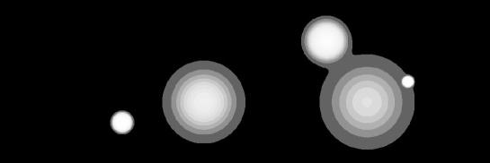
Figure 3: Visualization of the artificial structure defined from 5 different Gaussian distributions, before noise was added. Data array dimensions: $1200\times 400$ (portrayed transposed here).

We generated structure by placing Gaussians centered at the following row, column locations in a $1200\times 400$ data array: 300,100; 800,300; 1000,200; 500,150; 900,150. These bivariate Gaussians were of total 10 units in each case. A full width at half maximum (equal to 2.35482 times the standard deviation of a Gaussian), was used in each case, respectively: 20, 50, 10, 100, 125. We will call this the data array containing structure. Figure 3 shows a schematic view of it. Next we added uniformly distributed random noise, where the values in the former (Gaussians) data set scaled down by a constant factor of 10. Figure 4 shows the data set we will now work on. (We added noise in order to have a non-trivial data set for our compressibility experiments.)

LARGE FIGURE NOT DISPLAYED: SEE COPY OF PAPER AT http://www.cs.rhul.ac.uk/home/fionn/papers

Figure 4: Data array dimensions: $1200\times 400$ (portrayed transposed). Structure is visible, and added uniform nose.

In Murtagh et al. (2000) it was noted how row and column permuting of a data table allows application of any wavelet transform, where we take the data table as a 2-dimensional image. For a 3-way data array, a wavelet working on a 3-dimensional image volume is directly applicable. The difficulty in using an image processing technique on a data array is that (i) we must optimally permute data table rows and columns, which is known to be an NP-complete problem, or (ii) we must accept that each alternative data table row and column permutation will lead to a different result.

To exemplify this situation, we take the data generated as described above, which is by construction optimally row/column permuted. Figure 4 shows the data used, generated as having structure (i.e., contiguous similar values, which can still be visually appreciated) but also subject to additional uniformly distributed noise. The noise notwithstanding, there is still structure present in this data which can be exploited for compression purposes. We carried out assessments with the Lempel-Ziv run length encoding compression algorithm, which is used in the gzip command in Unix.

The data array of Figure 4 was of size 1,923,840 bytes. A random row/column permuted version of this array was of identical size. This random row/column permuting used uniformly distributed ranks. In all cases considered here, 32-bit floating point storage was used, and each array, stored as an image, contained a small additional ascii header.

Applying Lempel-Ziv compression to these data tables yielded gzip-compressed files of size, respectively, 1,720,368 and 1,721,284 bytes. There is not a great deal of compressibility present here. The row/column permutation, as expected, is not of help.

Next, we used our hierarchical wavelet transform, where the output is of exactly the same dimensions as our input (here: $1200\times 400$). Again we stored this transformed data in an image format, using 32-bit floating point storage. So the size of the transformed data was again exactly 1,923,840 bytes. This is irrespective of any wavelet filtering (by setting wavelet transform coefficients to 0), and is solely due to the file size, based on so much data, each value of which is stored as a 32-bit floating point value.

Then we compressed, using Lempel-Ziv, the wavelet transform data. We looked at three alternatives: no wavelet filtering used; wavelet filtering such that coefficients with value up to 0.05 were set to 0; and wavelet filtering such that coefficients with value up to 0.1 were set to 0.

The Lempel-Ziv compressed files were respectively of sizes: 1,780,912, 1,435,477, and 1,108,743 bytes. We see very clearly that Lempel-Ziv run length encoding is benefiting from our wavelet filtering, provided that there is sufficient filtering.

It is useful to proceed further with this study, to see if simple filtering, similar to what we are doing in wavelet space, can be applied also to the original data (or, for that matter, the permuted data).

HWT thresh.	MSE	Comp. size	Orig. thresh.	MSE	Comp. size
0	0	1,780,912	0	0	1,720,368
0.05	0.0032	1,435,477	0.25	0.0028	1,447,984
0.1	0.0119	1,108,743	0.39	0.0111	1,252,793

Table 6: Columns from left to right: Haar wavelet transform threshold applied to transformed data, with values lower than or equal to this set to 0; mean square error between input data and reconstructed, filtered data; compression size in bytes of the reconstructed, filtered data; threshold applied to the original data, with values lower than or equal to this set to 0; mean square error between input data and thresholded data; compression size in bytes of the thresholded data. See text for discussion.

Table 6 shows what we found. The mean square error (MSE) here is $\sum_{ij}(\hat{x}_{ij}-x_{ij})^{2}/\sum_{ij}x_{ij}^{2}$. What is noticeable is that in the 2nd and 3rd rows of the table processing the original data is seen to have better MSE coupled with worse compressibility. A fortiori we claim that for the same MSE we would have even worse compressibility.

Our wavelet approach therefore has performed better in this study than direct processing of the given data. Furthermore, relative to arbitrary permuting of the rows and columns, our given data represents a relatively favorable case. In practice, we have no guarantee that rows and columns are arranged such that like values are contiguous. But by design we have such a favorable situation here.

In concluding this study, we note the following work which uses a Fourier transform, rather than a wavelet transform, on a hierarchy or rooted tree. Kargupta and Park (2004) study the situation when a decision tree is given to begin with, and apply a Fourier transform to expedite compression. For our purposes, a hierarchical tree is determined in order to structure the data, and comprises the first part of a data processing pipeline. A subsequent part of the processing pipeline is the wavelet transform of the hierarchically structured data.

7 Wavelet-Based Multiway Tree Building: Approximating a Hierarchy by Tree Condensation

Deriving a partition from a hierarchical clustering has always been a crucial task in data analysis (an early example is Mojena, 1977). In this section we will explore a new approach to deriving a partition from a dendrogram. Deriving a partition from a dendrogram is equivalent to “collapsing” a strictly binary tree into a non-binary or multiway tree. Now, concept hierarchies are increasingly used to expedite search in information retrieval, especially in cross-disciplinary domains where a specification of the various terminologies used can be helpful to the user. For concept hierarchies, a non-binary or multiway tree is preferred for this purpose, and may, in practice, be determined from a binary tree (as do Chuang and Chien, 2005).

It is interesting to note that Lerman (1981, pp. 298–299) addresses this same issue of the “condensation of a tree to the levels corresponding to its significant nodes”, and then proceeds to discuss the global criterion used (for instance, in an agglomerative hierarchical algorithm) vis-à-vis a local criterion (where the latter is used to judge whether a node is significant or not). There is a clear parallel between this way of viewing the “collapsing clusters” problem and our way of tackling it.

A binary rooted tree, $H$, on $n$ observations has precisely $n-1$ levels; or $H$ contains precisely $n-1$ subsets of the set of $n$ observations. The interpretation of a hierarchical clustering often is carried out by cutting the tree to yield any one of the $n-1$ possible partitions. Our hierarchical Haar wavelet transform affords us a neat way to approximate $H$ using a smaller number of possible partitions.

Consider the detail vector at any given level: e.g., as exemplified in Table 2. Any such detail vector is associated with (i) a node of the binary tree; (ii) the level or height index of that node; and (iii) a cluster, or subset of the observation set. With the goal of “collapsing” clusters, i.e. removing clusters that are not unduly valuable for interpretation, we will impose a hard threshold on each detail vector: If the norm of the detail vector is less than a user-specified threshold, then set all values of the detail vector to zero.

Other rules could be chosen, in particular rules related directly to the agglomerative clustering criterion used, but our choice of the thresholded norm is a reasonable one. Our norm-based rule is not directly related to the agglomerative criterion for the following reasons: (i) we seek a generic interpretative aid, rather than an optimal but criterion-specific rule; (ii) an optimal, criterion-specific rule would in any case be best addressed by studying the overall optimality measure rather than availing of the stepwise suboptimal hierarchical clustering; and (iii) from naturally occurring hierarchies, as occur in very high dimensional spaces (cf. Murtagh, 2004), the issue of an agglomerative criterion is not important.

Following use of the norm-based cluster collapsing rule, the representation of the reconstructed hierarchy is straightforward: the hierarchy’s level index is adjusted so that the previous level index additionally takes the place of the given level index. Examples discussed below will exemplify this.

Properties of the approach include the following:

1. Rather than misleading increase in agglomerative clustering value or level, we examine instead clusters (or nodes in the hierarchy).

2. This implies that we explore a cluster at a time, rather than a partition at a time. So the resulting retained clusters may well come from different original partitions.

3. We take a strictly binary (2-way, agglomeratively constructed) tree as input and determine a simplified, multiway tree as output.

4. A single scalar value filtering threshold – a user-set parameter – is used to derive this output, simplified, multiway tree from the input binary tree.

5. The filtering is carried out on the wavelet-transformed tree; and then the output, simplified tree is reconstructed from the wavelet transform values.

6. The filtering is carried out on each node (in wavelet space) in sequence. Hence the computational complexity is linear.

7. Upstream of the wavelet transform, and hierarchical clustering, we use correspondence analysis to take frequency of occurrence data input, apply appropriate normalization, and map the data of interest into an (unweighted) Euclidean space. (See Murtagh, 2005.)

8. Again upstream of the wavelet transform, for the binary tree we use minimal variance hierarchical clustering. This agglomerative criterion favors compact clusters.

9. Our hierarchical clustering accommodates weights on the input observables to be clustered. Based on the normalization used in the correspondence analysis, by design these weights here are constant.

7.1 Properties of Derived Partition

A partition by definition is a set of clusters (sets) such that none are overlapping, and their union is the global set considered. So in Figure 5 the upper left hierarchy is cut, and shown in the lower left, to yield the partition consisting of clusters $(7,8,5,6),(1,2)$ and $(3,4)$. Traditionally, deriving such a partition for further exploitation is a common use of hierarchical clustering. Clearly the partition corresponds to a height or agglomeration threshold.

In a multiway hierarchy, such as the one shown in the top right panel in Figure 5, consider the same straight line drawn from left to right, at approximately the same height or agglomeration threshold. It is easily seen that such a partition is the same as that represented by the non-straight curve of the lower right panel.

From this illustrative example, we draw two conclusions: (i) in the case of a multiway tree a partition is furnished by a horizontal cut of the multiway tree – accomplished exactly as in the case of the strictly binary tree; and (ii) this horizontal cut of a multiway tree is identical to a nonlinear curve of the strictly binary tree. We can validly term the nonlinear curve a piecewise horizontal one.

Note that the nonlinear curve used in Figure 5, lower right panel, has nothing whatsoever to do with nonlinear cluster separation (in any ambient space in which the clusters are embedded), nor with nonlinear mapping.

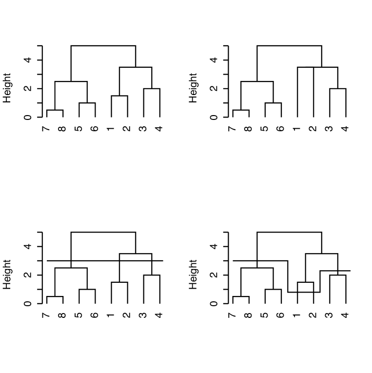
Figure 5: Upper left: original dendrogram. Upper right, multiway tree arising from one collapsed cluster or node. Lower left: a partition derived from the dendrogram (see text for discussion). Lower right: corresponding partition for the multiway tree.

7.2 Implementation and Evaluation

We took Aristotle’s Categories (see Aristotle, 350BC; Murtagh, 2005) in English containing 14,483 individual words. We broke up the text into 24 files, in order to study the sequential properties of the argument developed in this short philosophical work. In these 24 files, there were 1269 unique words. We selected 66 nouns of particular interest. With frequencies of occurrence in parentheses we had (sample only): man (104), contrary (72), same (71), subject (60), substance (58), species (54), knowledge (50), qualities (47), etc. No stemming or other preprocessing was applied on the grounds that singular and plurals could well indicate different semantic content; cf. generic “quantity” versus the set of specific, particular “quantities”.

The terms $\times$ subtexts data array was doubled (Murtagh, 2005) to produce a $66\times 48$ array: for each subtext $j$ with term frequencies of occurrence $a_{ij}$, frequencies from a “virtual subtext” were defined as $a^{\prime}_{ij}=\mbox{max}_{ij}\ a_{ij}-a_{ij}$. In this way the mass of term $i$, defined as proportional to the associated row sum, is constant. Thus what we have achieved is to weight all terms identically. (We note in passing that term vectors therefore cannot be of zero mass.)

A correspondence analysis was carried out on the $66\times 48$ table of frequencies with the aim of taking the set of 66 nouns endowed with the $\chi^{2}$ metric (i.e., a weighted Euclidean distance between profiles; the weighting is defined by the inverse subtext frequencies) into a factor space endowed with the (unweighted) Euclidean metric. (We note in passing that any subtexts of zero mass must be removed from the analysis beforehand; otherwise inverse subtext frequency cannot be calculated.) Correspondence analysis provides a convenient and general way to “euclideanize” the data, and any alternative could be considered also (e.g., as discussed in section 5.1 of Heiser, 2004). A hierarchical clustering (minimum variance method) was carried out on the factor coordinates of the 66 nouns. Such a hierarchical clustering is a strictly binary (i.e. 2-way), rooted tree.

The norms of detail vectors had minimum, median and maximum values as follows: 0.0758, 0.2440 and 0.6326, and these influenced the choice of threshold. Applying thresholds of 0, 0.2, 0.3 and 0.4 gave rise to the following numbers of “collapsed” clusters with, in brackets, the mean squared error between approximated data and original input data: 0 (0.0), 23 (0.0054), 44 (0.0147), and 55 (0.0164). Figure 6 shows the corresponding reconstructed and approximated hierarchies.

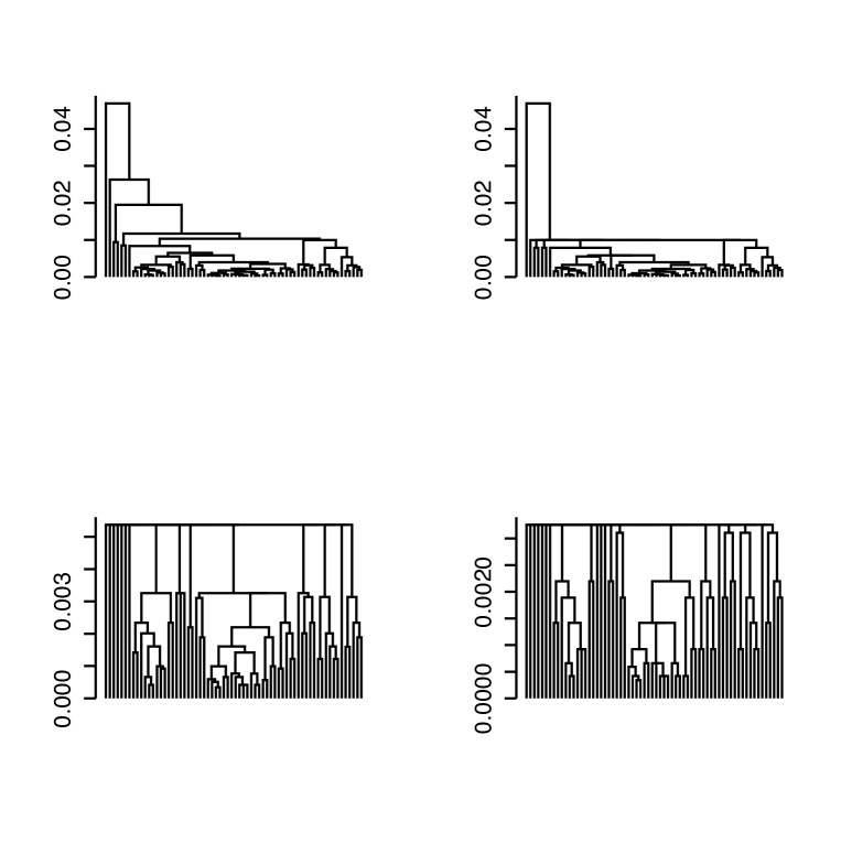
Figure 6: Upper left: original hierarchy. Upper right, lower left, and lower right show increasing approximations to the original hierarchy based on the “cluster collapsing” approach described.

In the case of the threshold 0.3 (lower left in Figure 6) we have noted that 44 clusters were collapsed, leaving just 21 partitions. As stated the objective here is precisely to approximate the dendrogram output data structure in order to facilitate further study and interpretation of these partitions.

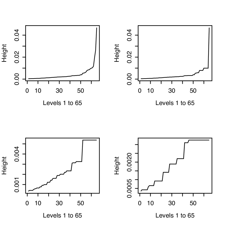
Figure 7: Agglomerative clustering levels (or heights) for each of the hierarchies shown in Figure 6.

Figure 7 shows the sequence of agglomerative levels where each panel corresponds to the respective panel in Figure 6. It is clear here why these agglomerative levels are very problematic if used for choosing a good partition: they increase with agglomeration, simply because the cluster centers are getting more and more spread out as the sequence of agglomerations proceeds. Directly using these agglomerative levels has been a way to derive a partition for a very long time (Mojena, 1977). To see how the detail norms used by us here are different, see Figure 8.

Figure 8: Agglomerative levels (left; as upper left in Figure 7, and corresponding to the original – upper left – hierarchy shown in Figure 6), and detail norms (right), for the hierarchy used. Detail norms are used by us as the basis for “collapsing clusters”.

7.3 Collapsing Clusters Based on Detail Norms: Evaluation Vis-à-vis Direct Partitioning

Our cluster collapsing algorithm is: wavelet-transform the hierarchical clustering; for clusters corresponding to detail norm less than a set threshold, set the detail norm to zero, and the corresponding increase in level in the hierarchy also; reconstruct the hierarchy. We look at a range of threshold values. To begin with, the hierarchical clustering is strictly binary. Reconstructed hierarchies are multiway.

For each unique level of such a multiway hierarchy (cf. Figure 6) how good are the partitions relative to a direct, optimization-based alternative? We use the algorithm of Hartigan and Wong (1979) with a requested number of clusters in the partition given by the same number of clusters in the collapsed cluster multiway hierarchy. In regard to the latter, we look at all unique partitions. (In regard to initialization and convergence criteria, the Hartigan and Wong algorithm implementation in the R package, www.r-project.org, was used.)

We characterize partitions using the average cluster variance,
$1/|Q|\sum_{i\in q;q\in Q}1/|q|\|i-q\|^{2}$. Alternatively we assessed the sum of squares: $\sum_{q\in Q}\|i-q\|^{2}$. Here, $Q$ is partition, $q$ is a cluster, and $\|i-q\|^{2}$ is Euclidean distance squared between a vector $i$ and its cluster center $q$. (Note that $q$ refers both to a set and to a cluster center – a vector – here.) Although this is a sum of squares criterion, as Späth (1985, p. 17) indicates, it is on occasion (confusingly) termed the variance criterion. In either case, we target compact clusters with this k-means clustering algorithm, which is also the target of our hierarchical agglomerative clustering algorithm. A k-means algorithm aims to optimize the criterion, in the Späth sense, directly.

In Table 7 we see that the partitions of our multiway hierarchy are about half as good as k-means in terms of overall compactness (cf. columns 3 and 5). Close inspection of properties of clusters in different partitions indicated why this was so: with a poor or low compactness for one cluster very early on in the agglomerative sequence, the stepwise algorithm used by the multiway hierarchy had to live with this cluster through all later agglomerations; and the biggest sized cluster (i.e. largest cluster cardinality) in the stepwise agglomerative tended to be a little bigger than the biggest sized cluster in the k-means result.

This is an acceptable result: after all, k-means optimizes this criterion directly. Furthermore, the multiway hierarchy preserves embededness relationships which are not necessarily present in any sequence of results ensuing from a k-means algorithm. Finally, it is well-known that seeking to directly optimize a criterion such as k-means will lead to a better outcome than the stepwise refinement used in the stepwise agglomerative algorithm.

If we ask whether k-means can be applied once, and then k-means applied to individual clusters in a recursive way, the answer is of course affirmative – subject to prior knowledge of the number of levels and the value of k throughout. It is precisely in such areas that our hierarchical approach is to be preferred: we require less prior knowledge of our data, and we are satisfied with the downside of global approximate fidelity between output structure and our data.

Agglom.	Multiway tree	Multiway tree	Partition	K-means
level	height	partition SS	cardinality	partition SS
1	0.00034	0.095	65	0.062
2	0.00042	0.229	61	0.091
3	0.00051	0.340	60	0.146
4	0.00057	0.397	59	0.205
5	0.00059	0.485	58	0.156
6	0.00066	0.739	55	0.239
7	0.00077	1.115	53	0.347
8	0.00092	1.447	51	0.484
9	0.00099	1.723	48	0.582
10	0.00122	2.329	45	0.852
11	0.00142	2.684	43	0.762
12	0.00159	3.101	42	0.865
13	0.00161	3.498	39	1.161
14	0.00189	3.938	36	1.354
15	0.00201	4.954	32	1.873
16	0.00220	5.293	30	2.178
17	0.00234	6.957	25	3.007
18	0.00311	7.204	24	2.722
19	0.00314	8.627	21	3.497
20	0.00326	10.192	15	5.426
21	0.00537	18.287	1	18.287

Table 7: Analysis of the unique partitions in the multiway tree shown on the lower left of Figure 6. Partitions are benchmarked using k-means to construct partitions where k is the same value as found in the multiway tree. SS = sum of squares criterion value.

8 Wavelet Decomposition: Linkages with Approximation and Computability

A further application of wavelet-transformed dendrograms is currently under investigation and will be briefly described here.

In domain theory (see Edalat, 1997; 2003), a Scott model considers a computer program as a function from one (input) domain to another (output) domain. If this function is continuous then the computation is well-defined and feasible, and the output is said to be computable. The Scott model is concerned with real number computation, or computer graphics programming where, e.g., object overlap may be true, false, or unknown and hence best modeled with a partially ordered set. In the Scott model, well-behaved approximation can benefit therefore from function monotonicity.

An alternative, although closely related, structure with which domains are endowed is that of spherically complete ultrametric spaces. The motivation comes from logic programming, where non-monotonicity may well be relevant (this arises, for example, with the negation operator). Trees can easily represent positive and negative assertions. The general notion of convergence, now, is related to spherical completeness (Schikhof, 1984; Hitzler and Seda, 2002). If we have any set of embedded clusters, or any chain, $q_{k}$, then the condition that such a chain be non-empty, $\bigcap_{k}q_{k}\neq\emptyset$, means that this ultrametric space is non-empty. This gives us both a concept of completeness, and also a fixed point which is associated with the “best approximation” of the chain.

Consider our space of observations, $X=\{x_{i}|i\in I\}$. The hierarchy, $H$, or binary rooted tree, defines an ultrametric space. For each observation $x_{i}$, by considering the chain from root cluster to the observation, we see that $H$ is a spherically complete ultrametric space.

Our wavelet transform allows us to read off the chains that make the ultrametric space a spherically complete one. A non-deterministic worst case $O(n)$ data re-creation algorithm ensues, compared to a more usual non-deterministic worst case $O(m)$ data recreation algorithm. The importance of this result is when $m>>n$.

In our current work (Murtagh, 2007) we are studying this perspective based on (i) a body of texts from the same author, and (ii) a library of face images.

9 Conclusion

We have described the theory and practice of a novel wavelet transform, that is based on an available hierarchic clustering of the data table. We have generally used Ward’s minimum variance agglomerative hierarchical clustering in this work.

We have described this new method through a number of examples, both to illustrate its properties and to show its operational use.

A number of innovative applications were undertaken with this new approach. These lead to various exciting open possibilities in regard to data mining, in particular in high dimensional spaces.

References

ALTAISKY, M.V. (2004). “p-Adic Wavelet Transform and Quantum Physics”, Proc. Steklov Institute of Mathematics, vol. 245, 34–39.

ALTAISKY, M.V. (2005). Wavelets: Theory, Applications, Implementation, Universities Press.

ARISTOTLE (350 BC). The Categories. Translated by E.M. Edghill. Project Gutenberg e-text, www.gutenberg.net

BENEDETTO, R.L. (2004). “Examples of Wavelets for Local Fields”, In C. Heil, P. Jorgensen, D. Larson, eds., Wavelets, Frames, and Operator Theory, Contemporary Mathematics Vol. 345, 27–47.

BENEDETTO, J.J. and BENEDETTO, R.L. (2004). “A Wavelet Theory for Local Fields and Related Groups”, The Journal of Geometric Analysis, 14, 423–456.

BENZÉCRI, J.P. (1979). La Taxinomie, 2nd ed., Paris: Dunod.

CHAKRABARTI, K., GAROFALAKIS, M., RASTOGI, R. and SHIM, K. (2001). “Approximate Query Processing using Wavelets”, VLDB Journal, International Journal on Very Large Databases, 10, 199–223.

SHUI-LUNG CHUANG and LEE-FENG CHIEN (2005). “Taxonomy Generation for Text Segments: A Practical Web-Based Approach”, ACM Transactions on Information Systems, 23, 363–396.

DEBNATH, L. and MIKUSIŃSKI, P. (1999). Introduction to Hilbert Spaces with Applications, 2nd edn., Academic Press.

EDALAT, A. (1997). “Domains for Computation in Mathematics, Physics and Exact Real Arithmetic”, Bulletin of Symbolic Logic, 3, 401–452.

EDALAT, A. (2003). “Domain Theory and Continuous Data Types”, lecture notes, www.doc.ic.ac.uk/$\sim$ae/teaching.html

FISHER, R.A. (1936). “The Use of Multiple Measurements in Taxonomic Problems”, The Annals of Eugenics, 7, 179–188.

FOOTE, R., MIRCHANDANI, G., ROCKMORE, D., HEALY, D. and OLSON, T. (2000a). “A Wreath Product Group Approach to Signal and Image Processing: Part I – Multiresolution Analysis”, IEEE Transactions on Signal Processing, 48, 102–132

FOOTE, R., MIRCHANDANI, G., ROCKMORE, D., HEALY, D. and OLSON, T. (2000b). “A Wreath Product Group Approach to Signal and Image Processing: Part II – Convolution, Correlations and Applications”, IEEE Transactions on Signal Processing, 48, 749–767.

FOOTE, R. (2005). “An Algebraic Approach to Multiresolution Analysis”, Transactions of the American Mathematical Society, 357, 5031–5050.

FRAZIER, M.W. (1999). An Introduction to Wavelets through Linear Algebra, New York: Springer.

HÄRDLE, W. (2000). Wavelets, Approximation, and Statistical Applications, Berlin: Springer.

HARTIGAN, J.A. and WONG, M.A. (1979). “A K-Means Clustering Algorithm”, Applied Statistics, 28, 100–108.

HEISER, W.J. (2004). “Geometric Representation of Association between Categories”, Psychometrika, 69, 513–545.

HITZLER, P. and SEDA, A.K. (2002). “The Fixed-Point Theorems of Priess-Crampe and Ribenboim in Logic Programming”, Fields Institute Communications, 32, 219–235.

JOE, M.J., WANG, K.-Y. and KIM, S.-W. (2001). “Wavelet Transformation-Based Management of Integrated Summary Data for Distributed Query Processing”, Data and Knowledge Engineering, 39, 293–312.

JOHNSON, S.C. (1967). “Hierarchical Clustering Schemes”, Psychometrika, 32, 241–254.

KARGUPTA, H. and PARK, B.-H. (2004). “A Fourier Spectrum-Based Approach to Represent Decision Trees for Mining Data Streams in Mobile Environments”, IEEE Transactions on Knowledge and Data Engineering, 16, 216–229.

KHRENNIKOV, A.Yu. and KOZYREV, S.V. (2006), “Ultrametric Random Field”, http://arxiv.org/abs/math.PR/0603584

KOZYREV, S.V. (2002). “Wavelet Analysis as a p-Adic Spectral Analysis”, Math. Izv., 66, 367–376. http://arxiv.org/abs/math-ph/0012019

KOZYREV, S.V. (2004). “P-Adic Pseudo-differential Operators and p-Adic Wavelets”, Theoretical and Mathematical Physics, 138, 322–332.

LERMAN, I.C. (1981). Classification et Analyse Ordinale des Données, Dunod.

MURTAGH, F. (1985). Multidimensional Clustering Algorithms, Würzburg: Physica-Verlag.

MURTAGH, F. (1998). “Wedding the Wavelet Transform and Multivariate Data Analysis”, Journal of Classification, 15, 161–183.

MURTAGH, F., STARCK, J.-L. and BERRY, M. (2000). “Overcoming the Curse of Dimensionality in Clustering by Means of the Wavelet Transform”, The Computer Journal, 43, 107–120.

MURTAGH, F. (2004). “On Ultrametricity, Data Coding, and Computation”, Journal of Classification, 21, 167–184.

MURTAGH, F. (2005). Correspondence Analysis and Data Coding with Java and R, Chapman and Hall.

MURTAGH, F. (2006). “Haar Wavelet Transform of a Dendrogram: Additional Notes”,
http://www.cs.rhul.ac.uk/home/fionn/papers/HWTden_notes.pdf

MURTAGH, F. (2007). “On ultrametric algorithmic information”, in preparation.

NABBEN, R. and VARGA, R.S. (1994). “A Linear Algebra Proof that the Inverse of a Strictly Ultrametric Matrix is a Strictly Diagonal Dominant Stieltjes Matrix”, SIAM Journal on Matrix Analysis and Applications, 15, 107–113.

OCKERBLOOM, J.M. (2003). Grimms’ Fairy Tales,
http://www.cs.cmu.edu/$\sim$spok/grimmtmp

SCHIKHOF, W.M. (1984). Ultrametric Calculus, Cambridge University Press.

SPÄTH, H. (1985). Cluster Dissection and Analysis, Ellis Horwood.

STARCK. J.-L. and MURTAGH, F. (2006). Astronomical Image and Data Analysis, Heidelberg: Springer. Chapter 9: “Multiple Resolution in Data Storage and Retrieval”. (1st edn., 2002.)

STRANG, G. and NGUYEN, T. (1996). Wavelets and Filter Banks, Wellesley-Cambridge Press.

TAO LI, QI LI, SHENGHUO ZHU, and MITSUNORI OGIHARA (2002). “A Survey on Wavelet Applications in Data Mining”, SIGKDD Explorations, 4, 49–68.

VITTER, J.S. and WANG, M. (1999). “Approximate Computation of Multidimensional Aggregates of Sparse Data using Wavelets”, in Proceedings of the ACM SIGMOD International Conference on Management of Data, 193–204.