Heap Reference Analysis Using Access Graphs

Abstract

Despite significant progress in the theory and practice of program analysis, analyzing properties of heap data has not reached the same level of maturity as the analysis of static and stack data. The spatial and temporal structure of stack and static data is well understood while that of heap data seems arbitrary and is unbounded. We devise bounded representations which summarize properties of the heap data. This summarization is based on the structure of the program which manipulates the heap. The resulting summary representations are certain kinds of graphs called access graphs. The boundedness of these representations and the monotonicity of the operations to manipulate them make it possible to compute them through data flow analysis.

An important application which benefits from heap reference analysis is garbage collection, where currently liveness is conservatively approximated by reachability from program variables. As a consequence, current garbage collectors leave a lot of garbage uncollected, a fact which has been confirmed by several empirical studies. We propose the first ever end-to-end static analysis to distinguish live objects from reachable objects. We use this information to make dead objects unreachable by modifying the program. This application is interesting because it requires discovering data flow information representing complex semantics. In particular, we formulate the following new analyses for heap data: liveness, availability, and anticipability and propose solution methods for them. Together, they cover various combinations of directions of analysis (i.e. forward and backward) and confluence of information (i.e. union and intersection). Our analysis can also be used for plugging memory leaks in C/C++ languages.

1 Introduction

Conceptually, data in a program is allocated in either the static data area, stack, or heap. Despite significant progress in the theory and practice of program analysis, analyzing the properties of heap data has not reached the same level of maturity as the analysis of static and stack data. Section 1.2 investigates possible reasons.

In order to facilitate a systematic analysis, we devise bounded representations which summarize properties of the heap data. This summarization is based on the structure of the program which manipulates the heap. The resulting summary representations are certain kinds of graphs, called access graphs which are obtained through data flow analysis. We believe that our technique of summarization is general enough to be also used in contexts other than heap reference analysis.

1.1 Improving Garbage Collection through Heap Reference Analysis

An important application which benefits from heap reference analysis is garbage collection, where liveness of heap data is conservatively approximated by reachability. This amounts to approximating the future of an execution with its past. Since current garbage collectors cannot distinguish live data from data that is reachable but not live, they leave a lot of garbage uncollected. This has been confirmed by empirical studies [Hirzel et al. (2002), Hirzel et al. (2002), Shaham et al. (2000), Shaham et al. (2001), Shaham et al. (2002)] which show that a large number (24% to 76%) of heap objects which are reachable at a program point are actually not accessed beyond that point. In order to collect such objects, we perform static analyses to make dead objects unreachable by setting appropriate references to null. The idea that doing so would facilitate better garbage collection is well known as “Cedar Mesa Folk Wisdom” [(13)]. The empirical attempts at achieving this have been [Shaham et al. (2001), Shaham et al. (2002)].

Garbage collection is an interesting application for us because it requires discovering data flow information representing complex semantics. In particular, we need to discover four properties of heap references: liveness, aliasing, availability, and anticipability. Liveness captures references that may be used beyond the program point under consideration. Only the references that are not live can be considered for null assignments. Safety of null assignments further requires (a) discovering all possible ways of accessing a given heap memory cell (aliasing), and (b) ensuring that the reference being nullified is accessible (availability and anticipability).

  $\begin{array}[]{ll}\\ 1.&w=x{\parbox{126.47249pt}{\raggedleft// $x$ points to $m_{a}$ \@add@raggedleft}}\\ 2.&\mbox{\em while }(x.getdata()<max)\\ &\{\\ 3.&\;\;\;\;\;\;\;\;x=x.\mbox{\em rptr\/}\\ &\}\\ 4.&y=x.\mbox{\em lptr\/}\\ 5.&z=\mbox{\em New }\mbox{\em class\_of\_z}\parbox{101.17755pt}{\raggedleft// Possible GC Point\@add@raggedleft}\\ 6.&y=y.\mbox{\em lptr\/}\\ 7.&z.sum=x.{\mbox{\em lptr\/}}.getdata()+y.getdata()\\ \\ \end{array}$ (a) A Program Fragment & $y=z=\mbox{\sf\em null\/}$ $y=z=\mbox{\sf\em null\/}$ 1. $w=x$ & $w=\mbox{\sf\em null\/}$ $w=\mbox{\sf\em null\/}$ 2. while $(x.getdata()<max)$ & {$\;\;\;\;\;\;x.\mbox{\em lptr\/}=\mbox{\sf\em null\/}$ {$\;\;\;\;\;\;x.\mbox{\em lptr\/}=\mbox{\sf\em null\/}$ 3. $\;\;\;\;\;\;\;\;\,x=x.\mbox{\em rptr\/}$ } & $x.\mbox{\em rptr\/}=x.\mbox{\em lptr\/}.\mbox{\em rptr\/}=\mbox{\sf\em null\/}$ $x.\mbox{\em lptr\/}.\mbox{\em lptr\/}.\mbox{\em lptr\/}=\mbox{\sf\em null\/}$ $x.\mbox{\em lptr\/}.\mbox{\em lptr\/}.\mbox{\em rptr\/}=\mbox{\sf\em null\/}$ $x.\mbox{\em rptr\/}=x.\mbox{\em lptr\/}.\mbox{\em rptr\/}=\mbox{\sf\em null\/}$ $x.\mbox{\em lptr\/}.\mbox{\em lptr\/}.\mbox{\em lptr\/}=\mbox{\sf\em null\/}$ $x.\mbox{\em lptr\/}.\mbox{\em lptr\/}.\mbox{\em rptr\/}=\mbox{\sf\em null\/}$ 4. $y=x.\mbox{\em lptr\/}$ & $y.\mbox{\em rptr\/}=y.\mbox{\em lptr\/}.\mbox{\em lptr\/}=y.\mbox{\em lptr\/}.\mbox{\em rptr\/}=\mbox{\sf\em null\/}$ $y.\mbox{\em rptr\/}=y.\mbox{\em lptr\/}.\mbox{\em lptr\/}=y.\mbox{\em lptr\/}.\mbox{\em rptr\/}=\mbox{\sf\em null\/}$ 5. $z$ = New class_of_z & $z.\mbox{\em lptr\/}=z.\mbox{\em rptr\/}=\mbox{\sf\em null\/}$ $z.\mbox{\em lptr\/}=z.\mbox{\em rptr\/}=\mbox{\sf\em null\/}$ 6. $y=y.\mbox{\em lptr\/}$ & $x.\mbox{\em lptr\/}.\mbox{\em lptr\/}=y.\mbox{\em lptr\/}=y.\mbox{\em rptr\/}=\mbox{\sf\em null\/}$ $x.\mbox{\em lptr\/}.\mbox{\em lptr\/}=y.\mbox{\em lptr\/}=y.\mbox{\em rptr\/}=\mbox{\sf\em null\/}$ 7. $z.sum=x.\mbox{\em lptr\/}.getdata()+y.getdata()$ & $x=y=z=\mbox{\sf\em null\/}$ $x=y=z=\mbox{\sf\em null\/}$ (c) The modified program. Highlighted statements indicate the null assignments inserted in the program using our method. (More details in Section 4)  

Figure 1: A motivating example.

For simplicity of exposition, we present our method using a memory model similar to that of Java. Extensions required for handling C/C++ model of heap usage are easy and are explained in Section 8. We assume that root variable references are on the stack and the actual objects corresponding to the root variables are in the heap. In the rest of the paper we ignore non-reference variables. We view the heap at a program point as a directed graph called memory graph. Root variables form the entry nodes of a memory graph. Other nodes in the graph correspond to objects on the heap and edges correspond to references. The out-edges of entry nodes are labeled by root variable names while out-edges of other nodes are labeled by field names. The edges in the memory graph are called links.

Example 1.1.

Figure 1 shows a program fragment and its memory graphs before line 5. Depending upon the number of times the while loop is executed $x$ points to $m_{a}$, $m_{b}$, $m_{c}$ etc. Correspondingly, $y$ points to $m_{i}$, $m_{f}$, $m_{g}$ etc. The call to New on line 5 may require garbage collection. A conventional copying collector will preserve all nodes except $m_{k}$. However, only a few of them are used beyond line 5.

The modified program is an evidence of the strength of our approach. It makes the unused nodes unreachable by nullifying relevant links. The modifications in the program are general enough to nullify appropriate links for any number of iterations of the loop. Observe that a null assignment has also been inserted within the loop body thereby making some memory unreachable in each iteration of the loop. $\Box$

After such modifications, a garbage collector will collect a lot more garbage. Further, since copying collectors process only live data, garbage collection by such collectors will be faster. Both these facts are corroborated by our empirical measurements (Section 7).

In the context of C/C++, instead of setting the references to null, allocated memory will have to be explicitly deallocated after checking that no alias is live.

1.2 Difficulties in Analyzing Heap Data

A program accesses data through expressions which have l-values and hence are called access expressions. They can be scalar variables such as $x$, or may involve an array access such as $a[2*i]$, or can be a reference expression such as $x.l.r$.

An important question that any program analysis has to answer is: Can an access expression $\alpha_{1}$ at program point $p_{1}$ have the same l-value as $\alpha_{2}$ at program point $p_{2}$? Note that the access expressions or program points could be identical. The precision of the analysis depends on the precision of the answer to the above question.

When the access expressions are simple and correspond to scalar data, answering the above question is often easy because, the mapping of access expressions to l-values remains fixed in a given scope throughout the execution of a program. However in the case of array or reference expressions, the mapping between an access expression and its l-value is likely to change during execution. From now on, we shall limit our attention to reference expressions, since these are the expressions that are primarily used to access the heap. Observe that manipulation of the heap is nothing but changing the mapping between reference expressions and their l-values. For example, in Figure 1, access expression $x.\mbox{\em lptr\/}$ refers to $m_{i}$ when the execution reaches line number 2 and may refer to $m_{i}$, $m_{f}$, $m_{g}$, or $m_{e}$ at line 4.

This implies that, subject to type compatibility, any access expression can correspond to any heap data, making it difficult to answer the question mentioned above. The problem is compounded because the program may contain loops implying that the same access expression appearing at the same program point may refer to different l-values at different points of time. Besides, the heap data may contain cycles, causing an infinite number of access expressions to refer to the same l-value. All these make analysis of programs involving heaps difficult.

1.3 Contributions of This Paper

The contributions of this paper fall in the following two categories

• Contributions in Data Flow Analysis. We present a data flow framework in which the data flow values represent abstractions of heap. An interesting aspect of our method is the way we obtain bounded representations of the properties by using the structure of the program which manipulates the heap. As a consequence of this summarization, the values of data flow information constitute a complete lattice with finite height. Further, we have carefully identified a set of monotonic operations to manipulate this data flow information. Hence, the standard results of data flow analysis can be extended to heap reference analysis. Due to the generality of this approach, it can be applied to other analyses as well.

• Contributions in Heap Data Analysis. We propose the first ever end-to-end solution (in the intraprocedural context) for statically discovering heap references which can be made null to improve garbage collection. The only approach which comes close to our approach is the heap safety automaton based approach [Shaham et al. (2003)]. However, our approach is superior to their approach in terms of completeness, effectiveness, and efficiency (details in Section 9.2).

The concept which unifies the contributions is the summarization of heap properties which uses the fact that the heap manipulations consist of repeating patterns which bear a close resemblance to the program structure. Our approach to summarization is more natural and more precise than other approaches because it does not depend on an a-priori bound [Jones and Muchnick (1979), Jones and Muchnick (1982), Larus and Hilfinger (1988), Chase et al. (1990)].

1.4 Organization of the paper

The rest of the paper is organized as follows. Section 2 defines the concept of explicit liveness of heap objects and formulates a data flow analysis by using access graphs as data flow values. Section 3 defines other properties required for ensuring safety of null assignment insertion. Section 4 explains how null assignments are inserted. Section 5 discusses convergence and complexity issues. Section 6 shows the soundness of our approach. Section 7 presents empirical results. Section 8 extends the approach to C++. Section 9 reviews related work while Section 10 concludes the paper.

2 Explicit Liveness Analysis of Heap References

Our method discovers live links at each program point, i.e., links which may be used in the program beyond the point under consideration. Links which are not live can be set to null. This section describes the liveness analysis. In particular, we define liveness of heap references, devise a bounded representation called an access graph for liveness, and then propose a data flow analysis for discovering liveness. Other analyses required for safety of null insertion are described in Section 3.

Our method is flow sensitive but context insensitive. This means that we compute point-specific information in each procedure by taking into account the flow of control at the intraprocedural level and by approximating the interprocedural information such that it is not context-specific but is safe in all calling contexts. For the purpose of analysis, arrays are handled by approximating any occurrence of an array element by the entire array. The current version models exception handling by explicating possible control flows. However, programs containing threads are not covered.

2.1 Access Paths

In order to discover liveness and other properties of heap, we need a way of naming links in the memory graph. We do this using access paths.

An access path is a root variable name followed by a sequence of zero or more field names and is denoted by $\rho_{x}\equiv x\mbox{\psset{unit=28.45276pt}\begin{pspicture}(0.0pt,0.0pt)(7.68224pt,5.69055pt){\psset{linewidth=0.42679pt}\psline(0.0pt,2.84528pt)(3.5566pt,2.84528pt)(3.5566pt,0.99583pt)(7.11319pt,2.84528pt)(3.5566pt,4.6947pt)(3.5566pt,2.84528pt)}\end{pspicture}}f_{1}\mbox{\psset{unit=28.45276pt}\begin{pspicture}(0.0pt,0.0pt)(7.68224pt,5.69055pt){\psset{linewidth=0.42679pt}\psline(0.0pt,2.84528pt)(3.5566pt,2.84528pt)(3.5566pt,0.99583pt)(7.11319pt,2.84528pt)(3.5566pt,4.6947pt)(3.5566pt,2.84528pt)}\end{pspicture}}f_{2}\mbox{\psset{unit=28.45276pt}\begin{pspicture}(0.0pt,0.0pt)(7.68224pt,5.69055pt){\psset{linewidth=0.42679pt}\psline(0.0pt,2.84528pt)(3.5566pt,2.84528pt)(3.5566pt,0.99583pt)(7.11319pt,2.84528pt)(3.5566pt,4.6947pt)(3.5566pt,2.84528pt)}\end{pspicture}}\cdots\mbox{\psset{unit=28.45276pt}\begin{pspicture}(0.0pt,0.0pt)(7.68224pt,5.69055pt){\psset{linewidth=0.42679pt}\psline(0.0pt,2.84528pt)(3.5566pt,2.84528pt)(3.5566pt,0.99583pt)(7.11319pt,2.84528pt)(3.5566pt,4.6947pt)(3.5566pt,2.84528pt)}\end{pspicture}}f_{k}$. Since an access path represents a path in a memory graph, it can be used for naming links and nodes. An access path consisting of just a root variable name is called a simple access path; it represents a path consisting of a single link corresponding to the root variable. $\mathcal{E}$ denotes an empty access path.

The last field name in an access path $\rho$ is called its frontier and is denoted by $\mbox{\sf\em Frontier\/}(\rho)$. The frontier of a simple access path is the root variable name. The access path corresponding to the longest sequence of names in $\rho$ excluding its frontier is called its base and is denoted by $\mbox{\sf\em Base\/}(\rho)$. Base of a simple access path is the empty access path $\mathcal{E}$. The object reached by traversing an access path $\rho$ is called the target of the access path and is denoted by $\mbox{\sf\em Target\/}(\rho)$. When we use an access path $\rho$ to refer to a link in a memory graph, it denotes the last link in $\rho$, i.e. the link corresponding to $\mbox{\sf\em Frontier\/}(\rho)$.

Example 2.1.

As explained earlier, Figure 1(b) is the superimposition of memory graphs that can result before line 5 for different executions of the program. For the access path $\rho_{x}\equiv x\mbox{\psset{unit=28.45276pt}\begin{pspicture}(0.0pt,0.0pt)(7.68224pt,5.69055pt){\psset{linewidth=0.42679pt}\psline(0.0pt,2.84528pt)(3.5566pt,2.84528pt)(3.5566pt,0.99583pt)(7.11319pt,2.84528pt)(3.5566pt,4.6947pt)(3.5566pt,2.84528pt)}\end{pspicture}}\mbox{\em lptr\/}\mbox{\psset{unit=28.45276pt}\begin{pspicture}(0.0pt,0.0pt)(7.68224pt,5.69055pt){\psset{linewidth=0.42679pt}\psline(0.0pt,2.84528pt)(3.5566pt,2.84528pt)(3.5566pt,0.99583pt)(7.11319pt,2.84528pt)(3.5566pt,4.6947pt)(3.5566pt,2.84528pt)}\end{pspicture}}\mbox{\em lptr\/}$, depending on whether the while loop is executed 0, 1, 2, or 3 times, $\mbox{\sf\em Target\/}(\rho_{x})$ denotes nodes $m_{j}$, $m_{h}$, $m_{m}$, or $m_{l}$. $\mbox{\sf\em Frontier\/}(\rho_{x})$ denotes one of the links $m_{i}\rightarrow m_{j}$, $m_{f}\rightarrow m_{h}$, $m_{g}\rightarrow m_{m}$ or $m_{e}\rightarrow m_{l}$. $\mbox{\sf\em Base\/}(\rho_{x})$ represents the following paths in the heap memory: $x\rightarrow m_{a}\rightarrow m_{i}$, $x\rightarrow m_{b}\rightarrow m_{f}$, $x\rightarrow m_{c}\rightarrow m_{g}$ or $x\rightarrow m_{d}\rightarrow m_{e}$. $\Box$

In the rest of the paper, $\alpha$ denotes an access expression, $\rho$ denotes an access path and $\sigma$ denotes a (possibly empty) sequence of field names separated by . Let the access expression $\alpha_{x}$ be $x.f_{1}.f_{2}\ldots f_{n}$. Then, the corresponding access path $\rho_{x}$ is $x\mbox{\psset{unit=28.45276pt}\begin{pspicture}(0.0pt,0.0pt)(7.68224pt,5.69055pt){\psset{linewidth=0.42679pt}\psline(0.0pt,2.84528pt)(3.5566pt,2.84528pt)(3.5566pt,0.99583pt)(7.11319pt,2.84528pt)(3.5566pt,4.6947pt)(3.5566pt,2.84528pt)}\end{pspicture}}f_{1}\mbox{\psset{unit=28.45276pt}\begin{pspicture}(0.0pt,0.0pt)(7.68224pt,5.69055pt){\psset{linewidth=0.42679pt}\psline(0.0pt,2.84528pt)(3.5566pt,2.84528pt)(3.5566pt,0.99583pt)(7.11319pt,2.84528pt)(3.5566pt,4.6947pt)(3.5566pt,2.84528pt)}\end{pspicture}}f_{2}\ldots f_{n}$. When the root variable name is not required, we drop the subscripts from $\alpha_{x}$ and $\rho_{x}$.

2.2 Program Flow Graph

Since the current version of our method involves context insensitive analysis, each procedure is analyzed separately and only once. Thus there is no need of maintaining a call graph and we use the term program and procedure interchangeably.

To simplify the description of analysis we make the following assumptions:

• The program flow graph has a unique Entry and a unique Exit node. We assume that there is a distinguished main procedure.

• Each statement forms a basic block.

• The conditions that alter flow of control are made up only of simple variables. If not, the offending reference expression is assigned to a fresh simple variable before the condition and is replaced by the fresh variable in the condition.

With these simplification, each statement falls in one of the following categories:

• Function Calls. These are statements $x=f(\alpha_{y},\alpha_{z},\ldots)$ where the functions involve access expressions in arguments. The type of $x$ does not matter.

• Assignment Statements. These are assignments to references and are denoted by $\alpha_{x}=\alpha_{y}$. Only these statements can modify the structure of the heap.

• Use Statements. These statements use heap references to access heap data but do not modify heap references. For the purpose of analysis, these statements are abstracted as lists of expressions $\alpha_{y}.d$ where $\alpha_{y}$ is an access expression and $d$ is a non-reference.

• Return Statement of the type $\mbox{\sf\em return\/}\;\alpha_{x}$ involving reference variable $x$.

• Other Statements. These statements include all statements which do not refer to the heap. We ignore these statements since they do not influence heap reference analysis.

When we talk about the execution path, we shall refer to the execution of the program derived by retaining all function calls, assignments and use statements and ignoring the condition checks in the path.

For simplicity of exposition, we present the analyses assuming that there are no cycles in the heap. This assumption does not limit the theory in any way because our analyses inherently compute conservative information in the presence of cycles without requiring any special treatment.

2.3 Liveness of Access Paths

A link $l$ is live at a program point $p$ if it is used in some control flow path starting from $p$. Note that $l$ may be used in two different ways. It may be dereferenced to access an object or tested for comparison. An erroneous nullification of $l$ would affect the two uses in different ways: Dereferencing $l$ would result in an exception being raised whereas testing $l$ for comparison may alter the result of condition and thereby the execution path.

Figure 1(b) shows links that are live before line 5 by thick arrows. For a link $l$ to be live, there must be at least one access path from some root variable to $l$ such that every link in this path is live. This is the path that is actually traversed while using $l$.

Since our technique involves nullification of access paths, we need to extend the notion of liveness from links to access paths. An access path is defined to be live at $p$ if the link corresponding to its frontier is live along some path starting at $p$. Safety of null assignments requires that the access paths which are live are excluded from nullification.

We initially limit ourselves to a subset of live access paths, whose liveness can be determined without taking into account the aliases created before $p$. These access paths are live solely because of the execution of the program beyond $p$. We call access paths which are live in this sense as explicitly live access paths. An interesting property of explicitly live access paths is that they form the minimal set covering every live link.

Example 2.2.

If the body of the while loop in Figure 1(a) is not executed even once, $\mbox{\sf\em Target\/}(y)=m_{i}$ at line 5 and the link $m_{i}\rightarrow m_{j}$ is live at line 5 because it is used in line 6. The access paths $y$ and $y\mbox{\psset{unit=28.45276pt}\begin{pspicture}(0.0pt,0.0pt)(7.68224pt,5.69055pt){\psset{linewidth=0.42679pt}\psline(0.0pt,2.84528pt)(3.5566pt,2.84528pt)(3.5566pt,0.99583pt)(7.11319pt,2.84528pt)(3.5566pt,4.6947pt)(3.5566pt,2.84528pt)}\end{pspicture}}\mbox{\em lptr\/}$ are explicitly live because their liveness at 5 can be determined solely from the statements from 5 onwards. In contrast, the access path $w\mbox{\psset{unit=28.45276pt}\begin{pspicture}(0.0pt,0.0pt)(7.68224pt,5.69055pt){\psset{linewidth=0.42679pt}\psline(0.0pt,2.84528pt)(3.5566pt,2.84528pt)(3.5566pt,0.99583pt)(7.11319pt,2.84528pt)(3.5566pt,4.6947pt)(3.5566pt,2.84528pt)}\end{pspicture}}\mbox{\em lptr\/}\mbox{\psset{unit=28.45276pt}\begin{pspicture}(0.0pt,0.0pt)(7.68224pt,5.69055pt){\psset{linewidth=0.42679pt}\psline(0.0pt,2.84528pt)(3.5566pt,2.84528pt)(3.5566pt,0.99583pt)(7.11319pt,2.84528pt)(3.5566pt,4.6947pt)(3.5566pt,2.84528pt)}\end{pspicture}}\mbox{\em lptr\/}$ is live without being explicitly live. It becomes live because of the alias between $y$ and $w\mbox{\psset{unit=28.45276pt}\begin{pspicture}(0.0pt,0.0pt)(7.68224pt,5.69055pt){\psset{linewidth=0.42679pt}\psline(0.0pt,2.84528pt)(3.5566pt,2.84528pt)(3.5566pt,0.99583pt)(7.11319pt,2.84528pt)(3.5566pt,4.6947pt)(3.5566pt,2.84528pt)}\end{pspicture}}\mbox{\em lptr\/}$ and this alias was created before 5. Also note that if an access path is explicitly live, so are all its prefixes. $\Box$

Example 2.3.

We illustrate the issues in determining explicit liveness of access paths by considering the assignment $x.r.n=y.n.n$.

• Killed Access Paths. Since the assignment modifies $\mbox{\sf\em Frontier\/}(x\mbox{\psset{unit=28.45276pt}\begin{pspicture}(0.0pt,0.0pt)(7.68224pt,5.69055pt){\psset{linewidth=0.42679pt}\psline(0.0pt,2.84528pt)(3.5566pt,2.84528pt)(3.5566pt,0.99583pt)(7.11319pt,2.84528pt)(3.5566pt,4.6947pt)(3.5566pt,2.84528pt)}\end{pspicture}}r\mbox{\psset{unit=28.45276pt}\begin{pspicture}(0.0pt,0.0pt)(7.68224pt,5.69055pt){\psset{linewidth=0.42679pt}\psline(0.0pt,2.84528pt)(3.5566pt,2.84528pt)(3.5566pt,0.99583pt)(7.11319pt,2.84528pt)(3.5566pt,4.6947pt)(3.5566pt,2.84528pt)}\end{pspicture}}n)$, any access path which is live after the assignment and has $x\mbox{\psset{unit=28.45276pt}\begin{pspicture}(0.0pt,0.0pt)(7.68224pt,5.69055pt){\psset{linewidth=0.42679pt}\psline(0.0pt,2.84528pt)(3.5566pt,2.84528pt)(3.5566pt,0.99583pt)(7.11319pt,2.84528pt)(3.5566pt,4.6947pt)(3.5566pt,2.84528pt)}\end{pspicture}}r\mbox{\psset{unit=28.45276pt}\begin{pspicture}(0.0pt,0.0pt)(7.68224pt,5.69055pt){\psset{linewidth=0.42679pt}\psline(0.0pt,2.84528pt)(3.5566pt,2.84528pt)(3.5566pt,0.99583pt)(7.11319pt,2.84528pt)(3.5566pt,4.6947pt)(3.5566pt,2.84528pt)}\end{pspicture}}n$ as prefix will cease to be live before the assignment. Access paths that are live after the assignment and not killed by it are live before the assignment also.

• Directly Generated Access Paths. All prefixes of $x\mbox{\psset{unit=28.45276pt}\begin{pspicture}(0.0pt,0.0pt)(7.68224pt,5.69055pt){\psset{linewidth=0.42679pt}\psline(0.0pt,2.84528pt)(3.5566pt,2.84528pt)(3.5566pt,0.99583pt)(7.11319pt,2.84528pt)(3.5566pt,4.6947pt)(3.5566pt,2.84528pt)}\end{pspicture}}r$ and $y\mbox{\psset{unit=28.45276pt}\begin{pspicture}(0.0pt,0.0pt)(7.68224pt,5.69055pt){\psset{linewidth=0.42679pt}\psline(0.0pt,2.84528pt)(3.5566pt,2.84528pt)(3.5566pt,0.99583pt)(7.11319pt,2.84528pt)(3.5566pt,4.6947pt)(3.5566pt,2.84528pt)}\end{pspicture}}n$ are explicitly live before the assignment due to the local effect of the assignment.

• Transferred Access Paths. If $x\mbox{\psset{unit=28.45276pt}\begin{pspicture}(0.0pt,0.0pt)(7.68224pt,5.69055pt){\psset{linewidth=0.42679pt}\psline(0.0pt,2.84528pt)(3.5566pt,2.84528pt)(3.5566pt,0.99583pt)(7.11319pt,2.84528pt)(3.5566pt,4.6947pt)(3.5566pt,2.84528pt)}\end{pspicture}}r\mbox{\psset{unit=28.45276pt}\begin{pspicture}(0.0pt,0.0pt)(7.68224pt,5.69055pt){\psset{linewidth=0.42679pt}\psline(0.0pt,2.84528pt)(3.5566pt,2.84528pt)(3.5566pt,0.99583pt)(7.11319pt,2.84528pt)(3.5566pt,4.6947pt)(3.5566pt,2.84528pt)}\end{pspicture}}n\mbox{\psset{unit=28.45276pt}\begin{pspicture}(0.0pt,0.0pt)(7.68224pt,5.69055pt){\psset{linewidth=0.42679pt}\psline(0.0pt,2.84528pt)(3.5566pt,2.84528pt)(3.5566pt,0.99583pt)(7.11319pt,2.84528pt)(3.5566pt,4.6947pt)(3.5566pt,2.84528pt)}\end{pspicture}}\sigma$ is live after the assignment, then $y\mbox{\psset{unit=28.45276pt}\begin{pspicture}(0.0pt,0.0pt)(7.68224pt,5.69055pt){\psset{linewidth=0.42679pt}\psline(0.0pt,2.84528pt)(3.5566pt,2.84528pt)(3.5566pt,0.99583pt)(7.11319pt,2.84528pt)(3.5566pt,4.6947pt)(3.5566pt,2.84528pt)}\end{pspicture}}n\mbox{\psset{unit=28.45276pt}\begin{pspicture}(0.0pt,0.0pt)(7.68224pt,5.69055pt){\psset{linewidth=0.42679pt}\psline(0.0pt,2.84528pt)(3.5566pt,2.84528pt)(3.5566pt,0.99583pt)(7.11319pt,2.84528pt)(3.5566pt,4.6947pt)(3.5566pt,2.84528pt)}\end{pspicture}}n\mbox{\psset{unit=28.45276pt}\begin{pspicture}(0.0pt,0.0pt)(7.68224pt,5.69055pt){\psset{linewidth=0.42679pt}\psline(0.0pt,2.84528pt)(3.5566pt,2.84528pt)(3.5566pt,0.99583pt)(7.11319pt,2.84528pt)(3.5566pt,4.6947pt)(3.5566pt,2.84528pt)}\end{pspicture}}\sigma$ will be live before the assignment. For example, if $x\mbox{\psset{unit=28.45276pt}\begin{pspicture}(0.0pt,0.0pt)(7.68224pt,5.69055pt){\psset{linewidth=0.42679pt}\psline(0.0pt,2.84528pt)(3.5566pt,2.84528pt)(3.5566pt,0.99583pt)(7.11319pt,2.84528pt)(3.5566pt,4.6947pt)(3.5566pt,2.84528pt)}\end{pspicture}}r\mbox{\psset{unit=28.45276pt}\begin{pspicture}(0.0pt,0.0pt)(7.68224pt,5.69055pt){\psset{linewidth=0.42679pt}\psline(0.0pt,2.84528pt)(3.5566pt,2.84528pt)(3.5566pt,0.99583pt)(7.11319pt,2.84528pt)(3.5566pt,4.6947pt)(3.5566pt,2.84528pt)}\end{pspicture}}n\mbox{\psset{unit=28.45276pt}\begin{pspicture}(0.0pt,0.0pt)(7.68224pt,5.69055pt){\psset{linewidth=0.42679pt}\psline(0.0pt,2.84528pt)(3.5566pt,2.84528pt)(3.5566pt,0.99583pt)(7.11319pt,2.84528pt)(3.5566pt,4.6947pt)(3.5566pt,2.84528pt)}\end{pspicture}}n$ is live after the assignment, then $y\mbox{\psset{unit=28.45276pt}\begin{pspicture}(0.0pt,0.0pt)(7.68224pt,5.69055pt){\psset{linewidth=0.42679pt}\psline(0.0pt,2.84528pt)(3.5566pt,2.84528pt)(3.5566pt,0.99583pt)(7.11319pt,2.84528pt)(3.5566pt,4.6947pt)(3.5566pt,2.84528pt)}\end{pspicture}}n\mbox{\psset{unit=28.45276pt}\begin{pspicture}(0.0pt,0.0pt)(7.68224pt,5.69055pt){\psset{linewidth=0.42679pt}\psline(0.0pt,2.84528pt)(3.5566pt,2.84528pt)(3.5566pt,0.99583pt)(7.11319pt,2.84528pt)(3.5566pt,4.6947pt)(3.5566pt,2.84528pt)}\end{pspicture}}n\mbox{\psset{unit=28.45276pt}\begin{pspicture}(0.0pt,0.0pt)(7.68224pt,5.69055pt){\psset{linewidth=0.42679pt}\psline(0.0pt,2.84528pt)(3.5566pt,2.84528pt)(3.5566pt,0.99583pt)(7.11319pt,2.84528pt)(3.5566pt,4.6947pt)(3.5566pt,2.84528pt)}\end{pspicture}}n$ will be live before the assignment. The sequence of field names $\sigma$ is viewed as being transferred from $x\mbox{\psset{unit=28.45276pt}\begin{pspicture}(0.0pt,0.0pt)(7.68224pt,5.69055pt){\psset{linewidth=0.42679pt}\psline(0.0pt,2.84528pt)(3.5566pt,2.84528pt)(3.5566pt,0.99583pt)(7.11319pt,2.84528pt)(3.5566pt,4.6947pt)(3.5566pt,2.84528pt)}\end{pspicture}}r\mbox{\psset{unit=28.45276pt}\begin{pspicture}(0.0pt,0.0pt)(7.68224pt,5.69055pt){\psset{linewidth=0.42679pt}\psline(0.0pt,2.84528pt)(3.5566pt,2.84528pt)(3.5566pt,0.99583pt)(7.11319pt,2.84528pt)(3.5566pt,4.6947pt)(3.5566pt,2.84528pt)}\end{pspicture}}n$ to $y\mbox{\psset{unit=28.45276pt}\begin{pspicture}(0.0pt,0.0pt)(7.68224pt,5.69055pt){\psset{linewidth=0.42679pt}\psline(0.0pt,2.84528pt)(3.5566pt,2.84528pt)(3.5566pt,0.99583pt)(7.11319pt,2.84528pt)(3.5566pt,4.6947pt)(3.5566pt,2.84528pt)}\end{pspicture}}n\mbox{\psset{unit=28.45276pt}\begin{pspicture}(0.0pt,0.0pt)(7.68224pt,5.69055pt){\psset{linewidth=0.42679pt}\psline(0.0pt,2.84528pt)(3.5566pt,2.84528pt)(3.5566pt,0.99583pt)(7.11319pt,2.84528pt)(3.5566pt,4.6947pt)(3.5566pt,2.84528pt)}\end{pspicture}}n$. $\Box$

We now define liveness by generalizing the above observations. We use the notation $\rho_{x}\mbox{\psset{unit=28.45276pt}\begin{pspicture}(0.0pt,0.0pt)(7.68224pt,5.69055pt){\psset{linewidth=0.42679pt}\psline(0.0pt,2.84528pt)(3.5566pt,2.84528pt)(3.5566pt,0.99583pt)(7.11319pt,2.84528pt)(3.5566pt,4.6947pt)(3.5566pt,2.84528pt)}\end{pspicture}}*$ to enumerate all access paths which have $\rho_{x}$ as a prefix. The summary liveness information for a set $S$ of reference variables is defined as follows:

$$\mbox{\em Summary\/}(S) = \bigcup_{x\in S}\{x\mbox{\psset{unit=28.45276pt}\begin{pspicture}(0.0pt,0.0pt)(7.68224pt,5.69055pt){\psset{linewidth=0.42679pt}\psline(0.0pt,2.84528pt)(3.5566pt,2.84528pt)(3.5566pt,0.99583pt)(7.11319pt,2.84528pt)(3.5566pt,4.6947pt)(3.5566pt,2.84528pt)}\end{pspicture}}*\}$$

Further, the set of all global variables is denoted by Globals  and the set of formal parameters of the function being analyzed is denoted by Params.

Definition 2.4.

Explicit Liveness. The set of explicitly live access paths at a program point $p$, denoted by $\mbox{\em Liveness\/}_{p}$ is defined as follows.

$$\mbox{\em Liveness\/}_{p} = \displaystyle\bigcup_{\psi\in Paths(p)}(\mbox{\em PathLiveness\/}^{\psi}_{p})$$

where, $\psi\in Paths(p)$ is a control flow path $p$ to Exit and $\mbox{\em PathLiveness\/}^{\psi}_{p}$ denotes the liveness at $p$ along $\psi$ and is defined as follows. If $p$ is not program exit then let the statement which follows it be denoted by $s$ and the program point immediately following $s$ be denoted by $p^{\prime}$. Then,

$$\mbox{\em PathLiveness\/}^{\psi}_{p} = \left\{\begin{array}[]{cl}\emptyset&p\mbox{ is \mbox{\sf\em Exit\/}\ of {\tt main}}\\ \ \mbox{\em Summary\/}(\mbox{\sf\em Globals\/})&p\mbox{ is \mbox{\sf\em Exit\/}\ of some procedure}\\ \mbox{\em StatementLiveness\/}_{s}(\mbox{\em PathLiveness\/}^{\psi}_{p^{\prime}})&\mbox{otherwise}\end{array}\right.$$

where the flow function for $s$ is defined as follows:

$$\mbox{\em StatementLiveness\/}_{s}(X) = (X-\mbox{$L{\mbox{\em Kill}}$}_{s})\;\cup\;\mbox{$L{\mbox{\em Direct}}$}_{s}\;\cup\;\mbox{$L{\mbox{\em Transfer}}$}_{s}(X)$$

$\mbox{$L{\mbox{\em Kill}}$}_{s}$ denotes the sets of access paths which cease to be live before statement $s$, $\mbox{$L{\mbox{\em Direct}}$}_{s}$ denotes the set of access paths which become live due to local effect of $s$ and $\mbox{$L{\mbox{\em Transfer}}$}_{s}(X)$ denotes the the set of access paths which become live before $s$ due to transfer of liveness from live access paths after $s$. They are defined in Figure 2. $\Box$

Observe that the definitions of $\mbox{$L{\mbox{\em Kill}}$}_{s}$, $\mbox{$L{\mbox{\em Direct}}$}_{s}$, and $\mbox{$L{\mbox{\em Transfer}}$}_{s}(X)$ ensure that the $\mbox{\em Liveness\/}_{p}$ is prefix-closed.

$\begin{array}[]{|l|c|c|c|}\hline\cr\mbox{Statement }s&\mbox{$L{\mbox{\em Kill}}$}_{s}&\mbox{$L{\mbox{\em Direct}}$}_{s}&\mbox{$L{\mbox{\em Transfer}}$}_{s}(X)\\ \hline\cr\hline\cr\alpha_{x}=\alpha_{y}&\{\rho_{x}\mbox{\psset{unit=28.45276pt}\begin{pspicture}(0.0pt,0.0pt)(7.68224pt,5.69055pt){\psset{linewidth=0.42679pt}\psline(0.0pt,2.84528pt)(3.5566pt,2.84528pt)(3.5566pt,0.99583pt)(7.11319pt,2.84528pt)(3.5566pt,4.6947pt)(3.5566pt,2.84528pt)}\end{pspicture}}*\}&(\mbox{\sf\em Base\/}(\rho_{x}))\cup(\mbox{\sf\em Base\/}(\rho_{y}))&\{\rho_{y}\mbox{\psset{unit=28.45276pt}\begin{pspicture}(0.0pt,0.0pt)(7.68224pt,5.69055pt){\psset{linewidth=0.42679pt}\psline(0.0pt,2.84528pt)(3.5566pt,2.84528pt)(3.5566pt,0.99583pt)(7.11319pt,2.84528pt)(3.5566pt,4.6947pt)(3.5566pt,2.84528pt)}\end{pspicture}}\sigma\mid\rho_{x}\mbox{\psset{unit=28.45276pt}\begin{pspicture}(0.0pt,0.0pt)(7.68224pt,5.69055pt){\psset{linewidth=0.42679pt}\psline(0.0pt,2.84528pt)(3.5566pt,2.84528pt)(3.5566pt,0.99583pt)(7.11319pt,2.84528pt)(3.5566pt,4.6947pt)(3.5566pt,2.84528pt)}\end{pspicture}}\sigma\in X\}\\ \hline\cr\alpha_{x}=f(\alpha_{y})&\{\rho_{x}\mbox{\psset{unit=28.45276pt}\begin{pspicture}(0.0pt,0.0pt)(7.68224pt,5.69055pt){\psset{linewidth=0.42679pt}\psline(0.0pt,2.84528pt)(3.5566pt,2.84528pt)(3.5566pt,0.99583pt)(7.11319pt,2.84528pt)(3.5566pt,4.6947pt)(3.5566pt,2.84528pt)}\end{pspicture}}*\}&(\mbox{\sf\em Base\/}(\rho_{x}))&\emptyset\\ &&\cup\;\mbox{\em Summary\/}(\{\rho_{y}\}\cup\mbox{\sf\em Globals\/})&\\ \hline\cr\alpha_{x}=\mbox{\sf\em new\/}&\{\rho_{x}\mbox{\psset{unit=28.45276pt}\begin{pspicture}(0.0pt,0.0pt)(7.68224pt,5.69055pt){\psset{linewidth=0.42679pt}\psline(0.0pt,2.84528pt)(3.5566pt,2.84528pt)(3.5566pt,0.99583pt)(7.11319pt,2.84528pt)(3.5566pt,4.6947pt)(3.5566pt,2.84528pt)}\end{pspicture}}*\}&(\mbox{\sf\em Base\/}(\rho_{x}))&\emptyset\\ \hline\cr\alpha_{x}=\mbox{\sf\em null\/}&\{\rho_{x}\mbox{\psset{unit=28.45276pt}\begin{pspicture}(0.0pt,0.0pt)(7.68224pt,5.69055pt){\psset{linewidth=0.42679pt}\psline(0.0pt,2.84528pt)(3.5566pt,2.84528pt)(3.5566pt,0.99583pt)(7.11319pt,2.84528pt)(3.5566pt,4.6947pt)(3.5566pt,2.84528pt)}\end{pspicture}}*\}&(\mbox{\sf\em Base\/}(\rho_{x}))&\emptyset\\ \hline\cr\mbox{\sf\em use\/}\;\alpha_{y}.d&\emptyset&(\rho_{y})&\emptyset\\ \hline\cr\mbox{\sf\em return\/}\;\alpha_{y}&\emptyset&\mbox{\em Summary\/}(\{\rho_{y}\})&\emptyset\\ \hline\cr\mbox{other}&\emptyset&\emptyset&\emptyset\\ \hline\cr\end{array}$

Figure 2: Defining Flow Functions for Liveness. Globals denotes the set of global references and Params denotes the set of formal parameters. For simplicity, we have shown a single access expression on the RHS.

 

Example 2.5.

In Figure 1, it cannot be statically determined which link is represented by access expression $x.\mbox{\em lptr\/}$ at line 4. Depending upon the number of iterations of the while loop, it may be any of the links represented by thick arrows. Thus at line 1, we have to assume that all access paths {$x\mbox{\psset{unit=28.45276pt}\begin{pspicture}(0.0pt,0.0pt)(7.68224pt,5.69055pt){\psset{linewidth=0.42679pt}\psline(0.0pt,2.84528pt)(3.5566pt,2.84528pt)(3.5566pt,0.99583pt)(7.11319pt,2.84528pt)(3.5566pt,4.6947pt)(3.5566pt,2.84528pt)}\end{pspicture}}\mbox{\em lptr\/}\mbox{\psset{unit=28.45276pt}\begin{pspicture}(0.0pt,0.0pt)(7.68224pt,5.69055pt){\psset{linewidth=0.42679pt}\psline(0.0pt,2.84528pt)(3.5566pt,2.84528pt)(3.5566pt,0.99583pt)(7.11319pt,2.84528pt)(3.5566pt,4.6947pt)(3.5566pt,2.84528pt)}\end{pspicture}}\mbox{\em lptr\/}$, $x\mbox{\psset{unit=28.45276pt}\begin{pspicture}(0.0pt,0.0pt)(7.68224pt,5.69055pt){\psset{linewidth=0.42679pt}\psline(0.0pt,2.84528pt)(3.5566pt,2.84528pt)(3.5566pt,0.99583pt)(7.11319pt,2.84528pt)(3.5566pt,4.6947pt)(3.5566pt,2.84528pt)}\end{pspicture}}\mbox{\em rptr\/}\mbox{\psset{unit=28.45276pt}\begin{pspicture}(0.0pt,0.0pt)(7.68224pt,5.69055pt){\psset{linewidth=0.42679pt}\psline(0.0pt,2.84528pt)(3.5566pt,2.84528pt)(3.5566pt,0.99583pt)(7.11319pt,2.84528pt)(3.5566pt,4.6947pt)(3.5566pt,2.84528pt)}\end{pspicture}}\mbox{\em lptr\/}\mbox{\psset{unit=28.45276pt}\begin{pspicture}(0.0pt,0.0pt)(7.68224pt,5.69055pt){\psset{linewidth=0.42679pt}\psline(0.0pt,2.84528pt)(3.5566pt,2.84528pt)(3.5566pt,0.99583pt)(7.11319pt,2.84528pt)(3.5566pt,4.6947pt)(3.5566pt,2.84528pt)}\end{pspicture}}\mbox{\em lptr\/}$, $x\mbox{\psset{unit=28.45276pt}\begin{pspicture}(0.0pt,0.0pt)(7.68224pt,5.69055pt){\psset{linewidth=0.42679pt}\psline(0.0pt,2.84528pt)(3.5566pt,2.84528pt)(3.5566pt,0.99583pt)(7.11319pt,2.84528pt)(3.5566pt,4.6947pt)(3.5566pt,2.84528pt)}\end{pspicture}}\mbox{\em rptr\/}\mbox{\psset{unit=28.45276pt}\begin{pspicture}(0.0pt,0.0pt)(7.68224pt,5.69055pt){\psset{linewidth=0.42679pt}\psline(0.0pt,2.84528pt)(3.5566pt,2.84528pt)(3.5566pt,0.99583pt)(7.11319pt,2.84528pt)(3.5566pt,4.6947pt)(3.5566pt,2.84528pt)}\end{pspicture}}\mbox{\em rptr\/}\mbox{\psset{unit=28.45276pt}\begin{pspicture}(0.0pt,0.0pt)(7.68224pt,5.69055pt){\psset{linewidth=0.42679pt}\psline(0.0pt,2.84528pt)(3.5566pt,2.84528pt)(3.5566pt,0.99583pt)(7.11319pt,2.84528pt)(3.5566pt,4.6947pt)(3.5566pt,2.84528pt)}\end{pspicture}}\mbox{\em lptr\/}\mbox{\psset{unit=28.45276pt}\begin{pspicture}(0.0pt,0.0pt)(7.68224pt,5.69055pt){\psset{linewidth=0.42679pt}\psline(0.0pt,2.84528pt)(3.5566pt,2.84528pt)(3.5566pt,0.99583pt)(7.11319pt,2.84528pt)(3.5566pt,4.6947pt)(3.5566pt,2.84528pt)}\end{pspicture}}\mbox{\em lptr\/}$, …} are explicitly live. $\Box$

In general, an infinite number of access paths with unbounded lengths may be live before a loop. Clearly, performing data flow analysis for access paths requires a suitable finite representation. Section 2.4 defines access graphs for the purpose.

2.4 Representing Sets of Access Paths by Access Graphs

In the presence of loops, the set of access paths may be infinite and the lengths of access paths may be unbounded. If the algorithm for analysis tries to compute sets of access paths explicitly, termination cannot be guaranteed. We solve this problem by representing a set of access paths by a graph of bounded size.

2.4.1 Defining Access Graphs

An access graph, denoted by $G_{v}$, is a directed graph $\langle n_{0},N,E\rangle$ representing a set of access paths starting from a root variable $v$. $N$ is the set of nodes, $n_{0}\in N_{F}$ is the entry node with no in-edges and $E$ is the set of edges. Every path in the graph represents an access path. The empty graph $\mbox{$\mathcal{E}$}\!_{G}$ has no nodes or edges and does not accept any access path.

The entry node of an access graphs is labeled with the name of the root variable while the non-entry nodes are labeled with a unique label created as follows: If a field name $f$ is referenced in basic block $b$, we create an access graph node with a label $\langle f,b,i\rangle$ where $i$ is the instance number used for distinguishing multiple occurrences of the field name $f$ in block $b$. Note that this implies that the nodes with the same label are treated as identical. Often, $i$ is 0 and in such a case we denote the label $\langle f,b,0\rangle$ by $f_{b}$ for brevity. Access paths $\rho_{x}\mbox{\psset{unit=28.45276pt}\begin{pspicture}(0.0pt,0.0pt)(7.68224pt,5.69055pt){\psset{linewidth=0.42679pt}\psline(0.0pt,2.84528pt)(3.5566pt,2.84528pt)(3.5566pt,0.99583pt)(7.11319pt,2.84528pt)(3.5566pt,4.6947pt)(3.5566pt,2.84528pt)}\end{pspicture}}*$ are represented by including a summary node denoted $n_{*}$ with a self loop over it. It is distinct from all other nodes but matches the field name of any other node.

A node in the access graph represents one or more links in the memory graph. Additionally, during analysis, it represents a state of access graph construction (explained in Section 2.4.2). An edge $f_{n}\rightarrow g_{m}$ in an access graph at program point $p$ indicates that a link corresponding to field $f$ dereferenced in block $n$ may be used to dereference a link corresponding to field $g$ in block $m$ on some path starting at $p$. This has been used in Section 5.2 to argue that the size of access graphs in practical programs is small.

Pictorially, the entry node of an access graph is indicated by an incoming double arrow.

Figure 3: Approximations in Access Graphs

 

2.4.2 Summarization

Recall that a link is live at a program point $p$ if it is used along some control flow path from $p$ to Exit. Since different access paths may be live along different control flow paths and there may be infinitely many control flow paths in the case of a loop following $p$, there may be infinitely many access paths which are live at $p$. Hence, the lengths of access paths will be unbounded. In such a case summarization is required.

Summarization is achieved by merging appropriate nodes in access graphs, retaining all in and out edges of merged nodes. We explain merging with the help of Figure 3:

• Node $n_{1}$ in access graph $G_{x}^{1}$ indicates references of $n$ at different execution instances of the same program point. Every time this program point is visited during analysis, the same state is reached in that the pattern of references after $n_{1}$ is repeated. Thus all occurrences of $n_{1}$ are merged into a single state. This creates a cycle which captures the repeating pattern of references.

• In $G_{x}^{2}$, nodes $n_{1}$ and $n_{2}$ indicate referencing $n$ at different program points. Since the references made after these program points may be different, $n_{1}$ and $n_{2}$ are not merged.

Summarization captures the pattern of heap traversal in the most straightforward way. Traversing a path in the heap requires the presence of reference assignments $\alpha_{x}=\alpha_{y}$ such that $\rho_{x}$ is a proper prefix of $\rho_{y}$. Assignments in Figure 3 are examples of such assignments. The structure of the flow of control between such assignments in a program determines the pattern of heap traversal. Summarization captures this pattern without the need of control flow analysis and the resulting structure is reflected in the access graphs as can be seen in Figure 3. More examples of the resemblance of program structure and access graph structure can be seen in the access graphs in Figure 6.

2.4.3 Operations on Access Graphs

Section 2.3 defined liveness by applying certain operations on access paths. In this subsection we define the corresponding operations on access graphs. Unless specified otherwise, the binary operations are applied only to access graphs having same root variable. The auxiliary operations and associated notations are:

• Root($\rho$) denotes the root variable of access path $\rho$, while Root($G$) denotes the root variable of access graph $G$.

• Field($n$) for a node $n$ denotes the field name component of the label of $n$.

• G$({\rho})$ constructs access graphs corresponding to $\rho$. It uses the current basic block number and the field names to create appropriate labels for nodes. The instance number depends on the number of occurrences of a field name in the block. G$({\rho\mbox{\psset{unit=28.45276pt}\begin{pspicture}(0.0pt,0.0pt)(7.68224pt,5.69055pt){\psset{linewidth=0.42679pt}\psline(0.0pt,2.84528pt)(3.5566pt,2.84528pt)(3.5566pt,0.99583pt)(7.11319pt,2.84528pt)(3.5566pt,4.6947pt)(3.5566pt,2.84528pt)}\end{pspicture}}*})$ creates an access graph with root variable $x$ and the summary node $n_{*}$ with an edge from $x$ to $n_{*}$ and a self loop over $n_{*}$.

• lastNode$({G})$ returns the last node of a linear graph $G$ constructed from a given $\rho$.

• $\mbox{\sf\em CleanUp\/}(G)$ deletes the nodes which are not reachable from the entry node.

• CN$({G},{G^{\prime}},{S})$ computes the set of nodes of $G$ which correspond to the nodes of $G^{\prime}$ specified in the set $S$. To compute CN$({G},{G^{\prime}},{S})$, we define ACN$({G},{G^{\prime}})$, the set of pairs of all corresponding nodes. Let $G\equiv\langle n_{0},N,E\rangle$ and $G^{\prime}\equiv\langle n^{\prime}_{0},N^{\prime},E^{\prime}\rangle$. A node $n$ in $G$ corresponds to a node $n^{\prime}$ in $G^{\prime}$ if there there exists an access path $\rho$ which is represented by a path from $n_{0}$ to $n$ in $G$ and a path from $n^{\prime}_{0}$ to $n^{\prime}$ in $G^{\prime}$.

  Formally, ACN$({G},{G^{\prime}})$ is the least solution of the following equation:

  ACN$$({G},{G^{\prime}}) = \left\{\begin{array}[]{llr@{}}\emptyset&&\hskip-28.45274pt\mbox{\sf\em Root\/}(G)\not=\mbox{\sf\em Root\/}(G^{\prime})\\ \{\langle n_{0},n^{\prime}_{0}\rangle\}\cup\{\langle n_{j},n^{\prime}_{j}\rangle\mid\mbox{\sf\em Field\/}(n_{j})=\mbox{\sf\em Field\/}(n^{\prime}_{j}),&&\mbox{otherwise}\\ {\hskip 85.35826pt}n_{i}\rightarrow n_{j}\in E,n^{\prime}_{i}\rightarrow n^{\prime}_{j}\in E^{\prime},\\ {\hskip 85.35826pt}\langle n_{i},n^{\prime}_{i}\rangle\ \in\mbox{{\sf\em ACN\/}$({G},{G^{\prime}})$}\}\end{array}\right.$$

  CN$$({G},{G^{\prime}},{S}) = \{n\mid\langle n,n^{\prime}\rangle\in\mbox{{\sf\em ACN\/}$({G},{G^{\prime}})$},\,n^{\prime}\in S\}$$

Note that $\mbox{\sf\em Field\/}(n_{j})=\mbox{\sf\em Field\/}(n^{\prime}_{j})$ would hold even when $n_{j}$ or $n^{\prime}_{j}$ is the summary node $n_{*}$.

Let $G\equiv\langle n_{0},N,E\rangle$ and $G^{\prime}\equiv\langle n_{0},N^{\prime},E^{\prime}\rangle$ be access graphs (having the same entry node). $G$ and $G^{\prime}$ are equal if $N=N^{\prime}$ and $E=E^{\prime}$.

The main operations of interest are defined below and are illustrated in Figure 4.

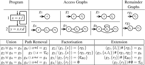
Figure 4: Examples of operations on access graphs.

 

1. Union (${\;\uplus\;}$). $G{\;\uplus\;}G^{\prime}$ combines access graphs $G$ and $G^{\prime}$ such that any access path contained in $G$ or $G^{\prime}$ is contained in the resulting graph.

   $$G{\;\uplus\;}G^{\prime} = \left\langle n_{0},N\cup N^{\prime},E\cup E^{\prime}\right\rangle$$

   The operation $N\cup N^{\prime}$ treats the nodes with the same label as identical. Because of associativity, ${\;\uplus\;}$ can be generalized to arbitrary number of arguments in an obvious manner.

2. Path Removal ($\ominus$). The operation $G\ominus\rho$ removes those access paths in $G$ which have $\rho$ as a prefix.

   $$G\ominus\rho = \left\{\begin{array}[]{ll}G&\rho=\mbox{$\mathcal{E}$}\mbox{ or }\mbox{\sf\em Root\/}(\rho)\neq\mbox{\sf\em Root\/}(G)\\ \mbox{$\mathcal{E}$}\!_{G}&\rho\mbox{ is a simple access path}\\ \mbox{\sf\em CleanUp\/}(\langle n_{0},N,E-E_{del}\rangle)\rule{8.5359pt}{0.0pt}&otherwise\end{array}\right.$$

   where

   $$\begin{array}[]{rcl}E_{del}&=&\{n_{i}\rightarrow n_{j}\mid n_{i}\rightarrow n_{j}\in E,n_{i}\in\mbox{{\sf\em CN\/}$({G},{G^{B}},{\{\mbox{{\sf\em lastNode\/}$({G^{B}})$}\}})$},\\ &&{\color[rgb]{1,1,1}\{n_{i}\mathop{\rightarrow}^{f}n_{j}\mid}\mbox{\sf\em Field\/}(n_{j})=\mbox{\sf\em Frontier\/}(\rho),G^{B}=\mbox{{\sf\em\small G\/}$({\mbox{\sf\em Base\/}(\rho)})$},\\ &&{\color[rgb]{1,1,1}\{n_{i}\mathop{\rightarrow}^{f}n_{j}\mid}\mbox{\sf\em UniqueAccessPath$\!$?\/}(G,n_{i})\}\end{array}$$

   UniqueAccessPath?($G$, $n$) returns true if in $G$, all paths from the entry node to node $n$ represent the same access path. Note that path removal is conservative in that some paths having $\rho$ as prefix may not be removed. Since an access graph edge may be contained in more than one access paths, we have to ensure that access paths which do not have $\rho$ as prefix are not erroneously deleted.

3. Factorization (/). Recall that the Transfer term in Definition 2.4 requires extracting suffixes of access paths and attaching them to some other access paths. The corresponding operations on access graphs are performed using factorization and extension. Given a node $m\in(N-\{n_{0}\})$ of an access graph $G$, the Remainder Graph of $G$ at $m$ is the subgraph of $G$ rooted at $m$ and is denoted by RG($G$, $m$). If $m$ does not have any outgoing edges, then the result is the empty remainder graph ${$\epsilon$}_{RG}$. Let $M$ be a subset of the nodes of $G^{\prime}$ and $M^{\prime}$ be the set of corresponding nodes in $G$. Then, $G/(G^{\prime},M)$ computes the set of remainder graphs of the successors of nodes in $M^{\prime}$.

   $$G/(G^{\prime},M) = \{\mbox{{\em RG}($G$, $n_{j}$)}\mid n_{i}\rightarrow n_{j}\in E,n_{i}\in\mbox{{\sf\em CN\/}$({G},{G^{\prime}},{M})$}\}$$ (4)

   A remainder graph is similar to an access graph except that (a) its entry node does not correspond to a root variable but to a field name and (b) the entry node can have incoming edges.

4. Extension. Extending an empty access graph $\mbox{$\mathcal{E}$}\!_{G}$ results in the empty access graph $\mbox{$\mathcal{E}$}\!_{G}$. For non-empty graphs, this operation is defined as follows.

   1. Extension with a remainder graph ($\cdot$). Let $M$ be a subset of the nodes of $G$ and $R\equiv\langle n^{\prime},\,N^{R},\,E^{R}\rangle$ be a remainder graph. Then, $(G,M)\cdot R$ appends the suffixes in $R$ to the access paths ending on nodes in $M$.

      $$(G,M)\cdot\mbox{${$\epsilon$}_{RG}$} = G$$

      $$(G,M)\cdot R = \left\langle n_{0},N\cup N^{R},E\cup E^{R}\cup\{n_{i}\rightarrow n^{\prime}\mid n_{i}\in M\}\right\rangle$$ (5)

   2. Extension with a set of remainder graphs ($\#$). Let $S$ be a set of remainder graphs. Then, $G\#\,S$ extends access graph $G$ with every remainder graph in $S$.

      $$(G,M)\#\,\emptyset = \mbox{$\mathcal{E}$}\!_{G}$$

      $$(G,M)\#\,S = \displaystyle\mathop{{\biguplus}}_{R\in S}\;\mbox{$(G,M)\cdot R$}$$ (6)

2.4.4 Safety of Access Graph Operations

$$\begin{array}[]{|l|l|l|}\hline\cr\mbox{Operation}&\mbox{Access Graphs}&\mbox{Access Paths}\\ \hline\cr\hline\cr\mbox{Union}&G_{3}=G_{1}{\;\uplus\;}\>G_{2}&\mbox{\sf\em P$({G_{3},M_{3}})$}\supseteq\mbox{\sf\em P$({G_{1},M_{1}})$}\cup\;\mbox{\sf\em P$({G_{2},M_{2}})$}\\ \hline\cr\mbox{Path Removal}&G_{2}=G_{1}\ominus\;\rho&\mbox{\sf\em P$({G_{2},M_{2}})$}\supseteq\mbox{\sf\em P$({G_{1},M_{1}})$}-\;\{\rho\mbox{\psset{unit=28.45276pt}\begin{pspicture}(0.0pt,0.0pt)(7.68224pt,5.69055pt){\psset{linewidth=0.42679pt}\psline(0.0pt,2.84528pt)(3.5566pt,2.84528pt)(3.5566pt,0.99583pt)(7.11319pt,2.84528pt)(3.5566pt,4.6947pt)(3.5566pt,2.84528pt)}\end{pspicture}}\sigma\mid\rho\mbox{\psset{unit=28.45276pt}\begin{pspicture}(0.0pt,0.0pt)(7.68224pt,5.69055pt){\psset{linewidth=0.42679pt}\psline(0.0pt,2.84528pt)(3.5566pt,2.84528pt)(3.5566pt,0.99583pt)(7.11319pt,2.84528pt)(3.5566pt,4.6947pt)(3.5566pt,2.84528pt)}\end{pspicture}}\sigma\in\mbox{\sf\em P$({G_{1},M_{1}})$}\}\\ \hline\cr\mbox{Factorization}&S=G_{1}/(G_{2},M)&\mbox{\sf\em P$({S,M_{s}})$}=\{\sigma\mid\rho^{\prime}\mbox{\psset{unit=28.45276pt}\begin{pspicture}(0.0pt,0.0pt)(7.68224pt,5.69055pt){\psset{linewidth=0.42679pt}\psline(0.0pt,2.84528pt)(3.5566pt,2.84528pt)(3.5566pt,0.99583pt)(7.11319pt,2.84528pt)(3.5566pt,4.6947pt)(3.5566pt,2.84528pt)}\end{pspicture}}\sigma\in\mbox{\sf\em P$({G_{1},M_{1}})$},\rho^{\prime}\in\mbox{\sf\em P$({G_{2},M})$}\}\\ \hline\cr\mbox{Extension}&G_{2}=\mbox{$(G_{1},M)\#\,S$}&\mbox{\sf\em P$({G_{2},M_{2}})$}\supseteq\mbox{\sf\em P$({G_{1},M_{1}})$}\cup\{\rho\mbox{\psset{unit=28.45276pt}\begin{pspicture}(0.0pt,0.0pt)(7.68224pt,5.69055pt){\psset{linewidth=0.42679pt}\psline(0.0pt,2.84528pt)(3.5566pt,2.84528pt)(3.5566pt,0.99583pt)(7.11319pt,2.84528pt)(3.5566pt,4.6947pt)(3.5566pt,2.84528pt)}\end{pspicture}}\sigma\mid\rho\in\mbox{\sf\em P$({G_{1},M})$},\sigma\in\mbox{\sf\em P$({S,M_{s}})$}\}\\ \hline\cr\end{array}$$

Figure 5: Safety of Access Graph Operations. P$({G,M})$ is the set of paths in graph $G$ terminating on nodes in $M$. For graph $G_{i}$, $M_{i}$ is the set of all nodes in $G_{i}$. $S$ is the set of remainder graphs and P$({S,M_{s}})$ is the set of all paths in all remainder graphs in $S$.

 

Since access graphs are not exact representations of sets of access paths, the safety of approximations needs to be defined explicitly. The constraints defined in Figure 5 capture safety in the context of liveness in the following sense: Every access path which can possibly be live should be retained by each operation. Since the complement of liveness is used for nullification, this ensures that no live access path is considered for nullification. These properties have been proved [Iyer (2005)] using the PVS theorem prover.

2.5 Data Flow Analysis for Discovering Explicit Liveness

For a given root variable $v$, $\mbox{{\sf E$\mathbb{L}$In}${}_{v}$}(i)$ and $\mbox{{\sf E$\mathbb{L}$Out}${}_{v}$}(i)$ denote the access graphs representing explicitly live access paths at the entry and exit of basic block $i$. We use $\mbox{$\mathcal{E}$}\!_{G}$ as the initial value for $\mbox{{\sf E$\mathbb{L}$In}${}_{v}$}(i)/\mbox{{\sf E$\mathbb{L}$Out}${}_{v}$}(i)$.

$$\mbox{{\sf E$\mathbb{L}$In}${}_{v}$}(i) = \left(\mbox{{\sf E$\mathbb{L}$Out}${}_{v}$}(i)\ominus\mbox{{\sf E$\mathbb{L}$KillPath}${}_{v}$}(i)\right){\;\uplus\;}\mbox{{\sf E$\mathbb{L}$Gen}${}_{v}$}(i)$$ (7)

$$\mbox{{\sf E$\mathbb{L}$Out}${}_{v}$}(i) = \left\{\begin{array}[]{l@{\ \ \ }l}\mbox{{\sf\em\small G\/}$({v\mbox{\psset{unit=28.45276pt}\begin{pspicture}(0.0pt,0.0pt)(7.68224pt,5.69055pt){\psset{linewidth=0.42679pt}\psline(0.0pt,2.84528pt)(3.5566pt,2.84528pt)(3.5566pt,0.99583pt)(7.11319pt,2.84528pt)(3.5566pt,4.6947pt)(3.5566pt,2.84528pt)}\end{pspicture}}*})$}&i=\mbox{\sf\em Exit\/},\;v\in\mbox{\sf\em Globals\/}\\ \mbox{$\mathcal{E}$}\!_{G}&i=\mbox{\sf\em Exit\/},\;v\not\in\mbox{\sf\em Globals\/}\\ \displaystyle\mathop{{\biguplus}}_{s\in succ(i)}\;\mbox{{\sf E$\mathbb{L}$In}${}_{v}$}(s)&\mbox{otherwise}\end{array}\right.$$ (11)

where

$$\mbox{{\sf E$\mathbb{L}$Gen}${}_{v}$}(i)=\mbox{\sf\em LDirect${}_{v}$}(i){\;\uplus\;}\mbox{\sf\em LTransfer${}_{v}$}(i)$$

We define $\mbox{{\sf E$\mathbb{L}$KillPath}${}_{v}$}(i)$, $\mbox{\sf\em LDirect${}_{v}$}(i)$, and $\mbox{\sf\em LTransfer${}_{v}$}(i)$ depending upon the statement.

1. Assignment statement $\alpha_{x}=\alpha_{y}$. Apart from defining the desired terms for $x$ and $y$, we also need to define them for any other variable $z$. In the following equations, $G_{x}$ and $G_{y}$ denote G$({\rho_{x}})$ and G$({\rho_{y}})$ respectively, whereas $M_{x}$ and $M_{y}$ denote lastNode$({\mbox{{\sf\em\small G\/}$({\rho_{x}})$}})$ and lastNode$({\mbox{{\sf\em\small G\/}$({\rho_{y}})$}})$ respectively.

   $$\mbox{\sf\em LDirect${}_{x}$}(i) \!\!=\!\! ({\mbox{\sf\em Base\/}(\rho_{x})})$$ G

   $$\mbox{\sf\em LDirect${}_{y}$}(i) \!\!=\!\! \left\{\!\!\begin{array}[]{l@{\ \ \ }l}\mbox{$\mathcal{E}$}\!_{G}&\alpha_{y}{\mbox{ is {\em New\/} \ldots\ or \mbox{\sf\em null\/}}}\\ \mbox{{\sf\em\small G\/}$({\mbox{\sf\em Base\/}(\rho_{y})})$}&\mbox{otherwise}\end{array}\right.$$ (14)

   $$\mbox{\sf\em LDirect${}_{z}$}(i) \!\!=\!\! \mbox{$\mathcal{E}$}\!_{G},\mbox{for any variable }z\mbox{ other than }x\mbox{ and }y$$

   $$\mbox{\sf\em LTransfer${}_{y}$}(i) \!\!=\!\! \left\{\!\!\begin{array}[]{l@{\ }l}\mbox{$\mathcal{E}$}\!_{G}&\alpha_{y}\mbox{ is {\em New\/} or \mbox{\sf\em null\/}}\\ \mbox{$(G_{y},M_{y})\#\,$}&\mbox{otherwise}\\ \;\;\;\;\;\;\;\;{(\mbox{{\sf E$\mathbb{L}$Out}${}_{x}$}(i)/(G_{x},M_{x}))}\end{array}\right.$$ (18)

   $$\mbox{\sf\em LTransfer${}_{z}$}(i) \!\!=\!\! \mbox{$\mathcal{E}$}\!_{G},\mbox{ for any variable }z\mbox{ other than }y$$

   $$\mbox{{\sf E$\mathbb{L}$KillPath}${}_{x}$}(i) \!\!=\!\! \rho_{x}$$

   $$\mbox{{\sf E$\mathbb{L}$KillPath}${}_{z}$}(i) \!\!=\!\! \mbox{$\mathcal{E}$},\mbox{ for any variable }z\mbox{ other than }x$$

   As stated earlier, the path removal operation deletes an edge only if it is contained in a unique path. Thus fewer paths may be killed than desired. This is a safe approximation. Another approximation which is also safe is that only the paths rooted at $x$ are killed. Since assignment to $\alpha_{x}$ changes the link represented by $\mbox{\sf\em Frontier\/}(\rho_{x})$, for precision, any path which is guaranteed to contain the link represented by $\mbox{\sf\em Frontier\/}(\rho_{x})$ should also be killed. Such paths can be discovered through must-alias analysis which we do not perform.

   

    

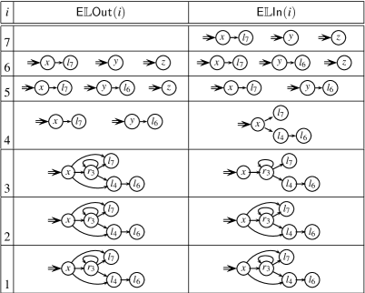
   Figure 6: Explicit liveness for the program in Figure 1 under the assumption that all variables are local variables.

2. Function call $\alpha_{x}=f(\alpha_{y})$. We conservatively assume that a function call may make any access path rooted at $y$ or any global reference variable live. Thus this version of our analysis is context insensitive.

   $$\mbox{\sf\em LDirect${}_{x}$}(i) \!\!=\!\! ({\mbox{\sf\em Base\/}(\rho_{x})})$$ G

   $$\mbox{\sf\em LDirect${}_{y}$}(i) \!\!=\!\! ({\rho_{y}\mbox{\psset{unit=28.45276pt}\begin{pspicture}(0.0pt,0.0pt)(7.68224pt,5.69055pt){\psset{linewidth=0.42679pt}\psline(0.0pt,2.84528pt)(3.5566pt,2.84528pt)(3.5566pt,0.99583pt)(7.11319pt,2.84528pt)(3.5566pt,4.6947pt)(3.5566pt,2.84528pt)}\end{pspicture}}*})$$ G

   $$\mbox{\sf\em LDirect${}_{z}$}(i) \!\!=\!\! \left\{\!\!\begin{array}[]{l@{\ }l}\mbox{{\sf\em\small G\/}$({z\mbox{\psset{unit=28.45276pt}\begin{pspicture}(0.0pt,0.0pt)(7.68224pt,5.69055pt){\psset{linewidth=0.42679pt}\psline(0.0pt,2.84528pt)(3.5566pt,2.84528pt)(3.5566pt,0.99583pt)(7.11319pt,2.84528pt)(3.5566pt,4.6947pt)(3.5566pt,2.84528pt)}\end{pspicture}}*})$}&\mbox{if $z$ is a global variable}\\ \mbox{$\mathcal{E}$}\!_{G}&\mbox{otherwise}\end{array}\right.$$

   $$\mbox{\sf\em LTransfer${}_{z}$}(i) \!\!=\!\! \mbox{$\mathcal{E}$}\!_{G},\mbox{ for all variables }z$$

   $$\mbox{{\sf E$\mathbb{L}$KillPath}${}_{x}$}(i) \!\!=\!\! \rho_{x}$$

   $$\mbox{{\sf E$\mathbb{L}$KillPath}${}_{z}$}(i) \!\!=\!\! \mbox{$\mathcal{E}$},\mbox{ for any variable }z\mbox{ other than }x$$

3. Return Statement $\mbox{\sf\em return\/}\;\alpha_{x}$.

   $$\mbox{\sf\em LDirect${}_{x}$}(i) \!\!=\!\! ({\rho_{x}\mbox{\psset{unit=28.45276pt}\begin{pspicture}(0.0pt,0.0pt)(7.68224pt,5.69055pt){\psset{linewidth=0.42679pt}\psline(0.0pt,2.84528pt)(3.5566pt,2.84528pt)(3.5566pt,0.99583pt)(7.11319pt,2.84528pt)(3.5566pt,4.6947pt)(3.5566pt,2.84528pt)}\end{pspicture}}*})$$ G

   $$\mbox{\sf\em LDirect${}_{z}$}(i) \!\!=\!\! \left\{\!\!\begin{array}[]{l@{\ }l}\mbox{{\sf\em\small G\/}$({z\mbox{\psset{unit=28.45276pt}\begin{pspicture}(0.0pt,0.0pt)(7.68224pt,5.69055pt){\psset{linewidth=0.42679pt}\psline(0.0pt,2.84528pt)(3.5566pt,2.84528pt)(3.5566pt,0.99583pt)(7.11319pt,2.84528pt)(3.5566pt,4.6947pt)(3.5566pt,2.84528pt)}\end{pspicture}}*})$}&\mbox{if $z$ is a global variable }\\ \mbox{$\mathcal{E}$}\!_{G}&\mbox{otherwise}\end{array}\right.$$

   $$\mbox{\sf\em LTransfer${}_{z}$}(i) \!\!=\!\! \mbox{$\mathcal{E}$}\!_{G},\mbox{ for any variable }z$$

   $$\mbox{{\sf E$\mathbb{L}$KillPath}${}_{z}$}(i) \!\!=\!\! \mbox{$\mathcal{E}$},\mbox{ for any variable }z$$

4. Use Statements

   $$\mbox{\sf\em LDirect${}_{x}$}(i) = {\biguplus}\;\mbox{{\sf\em\small G\/}$({\rho_{x}})$}\mbox{ \ for every }\alpha_{x}.d\mbox{ used in }i$$

   $$\mbox{\sf\em LDirect${}_{z}$}(i) = \mbox{$\mathcal{E}$}\!_{G}\mbox{ \ for any variable $z$ other than $x$ and}y$$

   $$\mbox{\sf\em LTransfer${}_{z}$}(i) = \mbox{$\mathcal{E}$}\!_{G},\mbox{ for every variable }z$$

   $$\mbox{{\sf E$\mathbb{L}$KillPath}${}_{z}$}(i) = \mbox{$\mathcal{E}$},\mbox{ for every variable }z$$

Example 2.6.

Figure 6 lists explicit liveness information at different points of the program in Figure 1 under the assumption that all variables are local variables. $\Box$

Observe that computing liveness using equations (7) and (11) results in an MFP (Maximum Fixed Point) solution of data flow analysis whereas definition (2.4) specifies an MoP (Meet over Paths) solution of data flow analysis. Since the flow functions are non-distributive (see appendix A), the two solutions may be different.

3 Other Analyses for Inserting null Assignments

Figure 7: Explicit liveness information is not sufficient for nullification.

 

Explicit liveness alone is not enough to decide whether an assignment $\alpha_{x}=\mbox{\sf\em null\/}$ can be safely inserted at $p$. We have to additionally ensure that:

• $\mbox{\sf\em Frontier\/}(\rho_{x})$ is not live through an alias created before the program point $p$. The extensions required to find all live access paths, including those created due to aliases, is discussed in section 3.1.

• Dereferencing links during the execution of the inserted statement $\alpha_{x}=\mbox{\sf\em null\/}$ does not cause an exception. This is done through availability and anticipability analysis and is described in section 3.2.

Both these requirements are illustrated through the example shown below:

Example 3.1.

In Figure 7, access path $y\mbox{\psset{unit=28.45276pt}\begin{pspicture}(0.0pt,0.0pt)(7.68224pt,5.69055pt){\psset{linewidth=0.42679pt}\psline(0.0pt,2.84528pt)(3.5566pt,2.84528pt)(3.5566pt,0.99583pt)(7.11319pt,2.84528pt)(3.5566pt,4.6947pt)(3.5566pt,2.84528pt)}\end{pspicture}}n$ is not explicitly live in block 6. However, $\mbox{\sf\em Frontier\/}(y\mbox{\psset{unit=28.45276pt}\begin{pspicture}(0.0pt,0.0pt)(7.68224pt,5.69055pt){\psset{linewidth=0.42679pt}\psline(0.0pt,2.84528pt)(3.5566pt,2.84528pt)(3.5566pt,0.99583pt)(7.11319pt,2.84528pt)(3.5566pt,4.6947pt)(3.5566pt,2.84528pt)}\end{pspicture}}n)$ and $\mbox{\sf\em Frontier\/}(x\mbox{\psset{unit=28.45276pt}\begin{pspicture}(0.0pt,0.0pt)(7.68224pt,5.69055pt){\psset{linewidth=0.42679pt}\psline(0.0pt,2.84528pt)(3.5566pt,2.84528pt)(3.5566pt,0.99583pt)(7.11319pt,2.84528pt)(3.5566pt,4.6947pt)(3.5566pt,2.84528pt)}\end{pspicture}}n)$ represent the same link due to the assignment $x=y$. Thus $y\mbox{\psset{unit=28.45276pt}\begin{pspicture}(0.0pt,0.0pt)(7.68224pt,5.69055pt){\psset{linewidth=0.42679pt}\psline(0.0pt,2.84528pt)(3.5566pt,2.84528pt)(3.5566pt,0.99583pt)(7.11319pt,2.84528pt)(3.5566pt,4.6947pt)(3.5566pt,2.84528pt)}\end{pspicture}}n$ is implicitly live and setting it to null in block 6 will raise an exception in block 7. Also, $x\mbox{\psset{unit=28.45276pt}\begin{pspicture}(0.0pt,0.0pt)(7.68224pt,5.69055pt){\psset{linewidth=0.42679pt}\psline(0.0pt,2.84528pt)(3.5566pt,2.84528pt)(3.5566pt,0.99583pt)(7.11319pt,2.84528pt)(3.5566pt,4.6947pt)(3.5566pt,2.84528pt)}\end{pspicture}}n\mbox{\psset{unit=28.45276pt}\begin{pspicture}(0.0pt,0.0pt)(7.68224pt,5.69055pt){\psset{linewidth=0.42679pt}\psline(0.0pt,2.84528pt)(3.5566pt,2.84528pt)(3.5566pt,0.99583pt)(7.11319pt,2.84528pt)(3.5566pt,4.6947pt)(3.5566pt,2.84528pt)}\end{pspicture}}n$ is not live in block 2. However, it cannot be set to null since the object pointed to by $x\mbox{\psset{unit=28.45276pt}\begin{pspicture}(0.0pt,0.0pt)(7.68224pt,5.69055pt){\psset{linewidth=0.42679pt}\psline(0.0pt,2.84528pt)(3.5566pt,2.84528pt)(3.5566pt,0.99583pt)(7.11319pt,2.84528pt)(3.5566pt,4.6947pt)(3.5566pt,2.84528pt)}\end{pspicture}}n$ does not exist in memory when the execution reaches block 2. Therefore, insertion of $x.n.n=\mbox{\sf\em null\/}$ in block 2 will raise an exception at run-time. $\Box$

3.1 Computing Live Access Paths

Recall that an access path is live if it is either explicitly live or shares its Frontier with some explicitly live path. The property of sharing is captured by aliasing. Two access paths $\rho_{x}$ and $\rho_{y}$ are aliased at a program point $p$ if $\mbox{\sf\em Target\/}(\rho_{x})$ is same as $\mbox{\sf\em Target\/}(\rho_{y})$ at $p$ during some execution of the program. They are link-aliased if their frontiers represent the same link; they are node-aliased if they are aliased but their frontiers do not represent the same link. Link-aliases can be derived from node-aliases (or other link-aliases) by adding the same field names to aliased access paths.

Alias information is flow-sensitive if the aliases at a program point depend on the statements along control flow paths reaching the point. Otherwise it is flow insensitive. Among flow sensitive aliases, two access paths are must-aliased at $p$ if they are aliased along every control flow path reaching $p$; they are may-aliased if they are aliased along some control flow path reaching $p$. As an example, in Figure 1, $x\mbox{\psset{unit=28.45276pt}\begin{pspicture}(0.0pt,0.0pt)(7.68224pt,5.69055pt){\psset{linewidth=0.42679pt}\psline(0.0pt,2.84528pt)(3.5566pt,2.84528pt)(3.5566pt,0.99583pt)(7.11319pt,2.84528pt)(3.5566pt,4.6947pt)(3.5566pt,2.84528pt)}\end{pspicture}}\mbox{\em lptr\/}$ and $y$ are must-node-aliases, $x\mbox{\psset{unit=28.45276pt}\begin{pspicture}(0.0pt,0.0pt)(7.68224pt,5.69055pt){\psset{linewidth=0.42679pt}\psline(0.0pt,2.84528pt)(3.5566pt,2.84528pt)(3.5566pt,0.99583pt)(7.11319pt,2.84528pt)(3.5566pt,4.6947pt)(3.5566pt,2.84528pt)}\end{pspicture}}\mbox{\em lptr\/}\mbox{\psset{unit=28.45276pt}\begin{pspicture}(0.0pt,0.0pt)(7.68224pt,5.69055pt){\psset{linewidth=0.42679pt}\psline(0.0pt,2.84528pt)(3.5566pt,2.84528pt)(3.5566pt,0.99583pt)(7.11319pt,2.84528pt)(3.5566pt,4.6947pt)(3.5566pt,2.84528pt)}\end{pspicture}}\mbox{\em lptr\/}$ and $y\mbox{\psset{unit=28.45276pt}\begin{pspicture}(0.0pt,0.0pt)(7.68224pt,5.69055pt){\psset{linewidth=0.42679pt}\psline(0.0pt,2.84528pt)(3.5566pt,2.84528pt)(3.5566pt,0.99583pt)(7.11319pt,2.84528pt)(3.5566pt,4.6947pt)(3.5566pt,2.84528pt)}\end{pspicture}}\mbox{\em lptr\/}$ are must-link-aliases, and $w$ and $x$ are node-aliases at line 5.

We compute flow sensitive may-aliases (without kills) using the algorithm described by hind99interprocedural and use pairs of access graphs for compact representation of aliases. Liveness is computed through a backward propagation much in the same manner as explicit liveness except that it is ensured that the live paths at each program point is closed under may-aliasing. This requires the following two changes in the earlier scheme.

1. Inclusion of Intermediate Nodes in Access Graphs. Unlike explicit liveness, live access paths may not be prefix closed. This is because the frontier of a live access path $\rho_{x}$ may be accessed using some other access path and not through the links which constitute $\rho_{x}$. Hence prefixes of $\rho_{x}$ may not be live. In an access graph representing liveness, all paths may not represent live links. We therefore modify the access graph so that such paths are not described by the access graph. In order to make this distinction, we divide the nodes in an access graphs in two categories: final and intermediate. The only access paths described by the access graph are those which end at final nodes. This change affects the access graph operations in the following manner:

   • The equality of graphs now must consider equality of the sets of intermediate nodes and the sets of final nodes separately.

   • Graph constructor G$({\rho_{x}})$ marks all nodes in the resulting graph as final implying that all non-empty prefixes of $\rho_{x}$ are contained in the graph. We define a new constructor GOnly$({\rho_{x}})$ which marks only the last node as final and all other nodes as intermediate implying that only $\rho_{x}$ is contained in the graph.

   • Whenever multiple nodes with identical labels are combined, if any instance of the node is final then the resulting node is treated as final. This influences union $(\!\!{\;\uplus\;}\!\!)$ and extension ($\#\,$).

   • The set $M$ used in defining factorization and extension (equations 4, 5, 6) and the safety properties of access graph operations (Figure 5) contain final nodes only.

   • Extension $G\cdot RG$ marks all nodes in $G$ as intermediate. If $G$ and $RG$ have a common node then the status of the node is governed by its status in $RG$.

   • The $\mbox{\sf\em CleanUp\/}(G)$ operation is modified to delete those intermediate nodes which do not have a path leading to a final node.

2. Link Alias Closure. To discover all link aliases of a live access we compute link alias closure as defined below. Given an alias set AS, the set of link aliases of an access path $\rho_{x}\mbox{\psset{unit=28.45276pt}\begin{pspicture}(0.0pt,0.0pt)(7.68224pt,5.69055pt){\psset{linewidth=0.42679pt}\psline(0.0pt,2.84528pt)(3.5566pt,2.84528pt)(3.5566pt,0.99583pt)(7.11319pt,2.84528pt)(3.5566pt,4.6947pt)(3.5566pt,2.84528pt)}\end{pspicture}}f$ is the least solution of:

   $$\mbox{\sf LnA}(\rho_{x}\mbox{\psset{unit=28.45276pt}\begin{pspicture}(0.0pt,0.0pt)(7.68224pt,5.69055pt){\psset{linewidth=0.42679pt}\psline(0.0pt,2.84528pt)(3.5566pt,2.84528pt)(3.5566pt,0.99583pt)(7.11319pt,2.84528pt)(3.5566pt,4.6947pt)(3.5566pt,2.84528pt)}\end{pspicture}}f,\mbox{\sf\em AS\/})=\{\rho_{y}\mbox{\psset{unit=28.45276pt}\begin{pspicture}(0.0pt,0.0pt)(7.68224pt,5.69055pt){\psset{linewidth=0.42679pt}\psline(0.0pt,2.84528pt)(3.5566pt,2.84528pt)(3.5566pt,0.99583pt)(7.11319pt,2.84528pt)(3.5566pt,4.6947pt)(3.5566pt,2.84528pt)}\end{pspicture}}f\mid\langle\rho_{x},\rho_{y}\rangle\in\mbox{\sf\em AS\/}\mbox{ or }\langle\rho_{x},\rho_{y}\rangle\in\mbox{\sf LnA}(\rho_{x},\mbox{\sf\em AS\/})\}$$

   Given an alias pair $\langle g_{x},g_{y}\rangle$ link aliases of $G_{x}$ rooted at $y$ are included in the access graph $G_{y}$ as follows:

   $$\mbox{\sf LnG}(G_{y},G_{x},\langle g_{x},g_{y}\rangle)=G_{y}{\;\uplus\;}\mbox{$(g_{y},m_{y})\#\,((G_{x}/(g_{x},m_{x})$})\!-\!\mbox{${$\epsilon$}_{RG}$})$$ (21)

   where $m_{y}$ and $m_{x}$ are the singleton sets containing the final nodes of $g_{y}$ and $g_{x}$ respectively. ${$\epsilon$}_{RG}$ has to be removed from set of remainder graphs because we want to transfer non-empty links only. Complete liveness is computed as the least solution of the following equations

   $$\mbox{{\sf$\mathbb{L}$In}${}_{v}$}(i) = \mbox{{\sf T$\mathbb{L}$In}${}_{v}$}(i)\displaystyle\mathop{{\biguplus}}_{\raisebox{0.28453pt}{$\scriptstyle\langle g_{v},g_{u}\rangle$}\in\raisebox{-0.56905pt}{\mbox{{\sf$\mathbb{A}$In}}(i)}}\mbox{\sf LnG}\left(\mbox{{\sf$\mathbb{L}$In}${}_{v}$}(i),\mbox{{\sf$\mathbb{L}$In}${}_{u}$}(i),\langle g_{v},g_{u}\rangle\right)$$

   $$\mbox{{\sf$\mathbb{L}$Out}${}_{v}$}(i) = \left\{\begin{array}[]{l@{\ \ \ }l}\mbox{{\sf\em\small G\/}$({v\mbox{\psset{unit=28.45276pt}\begin{pspicture}(0.0pt,0.0pt)(7.68224pt,5.69055pt){\psset{linewidth=0.42679pt}\psline(0.0pt,2.84528pt)(3.5566pt,2.84528pt)(3.5566pt,0.99583pt)(7.11319pt,2.84528pt)(3.5566pt,4.6947pt)(3.5566pt,2.84528pt)}\end{pspicture}}*})$}&i=\mbox{\sf\em Exit\/},\;v\in\mbox{\sf\em Globals\/}\\ &\mbox{or }v\in\mbox{\sf\em Params\/}\\ \mbox{$\mathcal{E}$}\!_{G}{\;\uplus\;}\mbox{\sf LnG}\left(\mbox{{\sf$\mathbb{L}$Out}${}_{v}$}(i),\mbox{{\sf$\mathbb{L}$Out}${}_{u}$}(i),\langle g_{v},g_{u}\rangle\right)&i=\mbox{\sf\em Exit\/},\;v\not\in\mbox{\sf\em Globals\/},\\ &\langle g_{v},g_{u}\rangle\in\mbox{{\sf$\mathbb{A}$Out}}(i)\\ \displaystyle\mathop{{\biguplus}}_{s\in succ(i)}\;\mbox{{\sf$\mathbb{L}$In}${}_{v}$}(s)&\mbox{otherwise}\end{array}\right.$$

   where $\mbox{{\sf T$\mathbb{L}$In}${}_{v}$}(i)$ is same as $\mbox{{\sf E$\mathbb{L}$In}${}_{v}$}(i)$ except that $\mbox{{\sf E$\mathbb{L}$Out}${}_{v}$}(i)$ is replaced by $\mbox{{\sf$\mathbb{L}$Out}${}_{v}$}(i)$ in the main equation (equation 7) and in the computation of Transfer (equation 18).

$$\begin{array}[]{|c|l|l|}\hline\cr i&\vrule\lx@intercol\hfil\mbox{{\sf$\mathbb{A}$In}}(i)\hfil\lx@intercol\vrule\lx@intercol&\vrule\lx@intercol\hfil\mbox{{\sf$\mathbb{A}$Out}}(i)\hfil\lx@intercol\vrule\lx@intercol\\ \hline\cr\hline\cr\rule[-7.5pt]{0.0pt}{20.00003pt}1&\vrule\lx@intercol\hfil\emptyset\hfil\lx@intercol\vrule\lx@intercol&\mbox{$\left\langle\raisebox{-3.69885pt}{{ {\psset{unit=2.27621pt} \begin{pspicture}(2.27621pt,0.56905pt)(20.48593pt,12.51918pt) { }{ } \rput(0.0pt,6.82864pt){\rnode{a}{}} { }{ } \rput(18.20972pt,6.82864pt){\rnode{x}{{\pscirclebox{$\,x\,$}}}} {\psset{doubleline=true}\ncline{->}{a}{x}} \end{pspicture} } } },\raisebox{-3.69885pt}{{ {\psset{unit=2.27621pt} \begin{pspicture}(2.27621pt,1.1381pt)(20.48593pt,12.51918pt) { }{ } \rput(0.0pt,6.82864pt){\rnode{a}{}} { }{ } \rput(18.20972pt,6.82864pt){\rnode{x}{{\pscirclebox{$w$}}}} {\psset{doubleline=true}\ncline{->}{a}{x}} \end{pspicture} } } }\right\rangle$}\\ \hline\cr\rule[-7.5pt]{0.0pt}{20.00003pt}2&\mbox{$\left\langle\raisebox{-3.69885pt}{{ {\psset{unit=2.27621pt} \begin{pspicture}(2.27621pt,0.56905pt)(20.48593pt,12.51918pt) { }{ } \rput(0.0pt,6.82864pt){\rnode{a}{}} { }{ } \rput(18.20972pt,6.82864pt){\rnode{x}{{\pscirclebox{$\,x\,$}}}} {\psset{doubleline=true}\ncline{->}{a}{x}} \end{pspicture} } } },\raisebox{-3.69885pt}{{ {\psset{unit=2.27621pt} \begin{pspicture}(2.27621pt,1.1381pt)(20.48593pt,12.51918pt) { }{ } \rput(0.0pt,6.82864pt){\rnode{a}{}} { }{ } \rput(18.20972pt,6.82864pt){\rnode{x}{{\pscirclebox{$w$}}}} {\psset{doubleline=true}\ncline{->}{a}{x}} \end{pspicture} } } }\right\rangle$},\mbox{$\left\langle\raisebox{-3.69885pt}{{ {\psset{unit=2.27621pt} \begin{pspicture}(2.27621pt,0.56905pt)(20.48593pt,12.51918pt) { }{ } \rput(0.0pt,6.82864pt){\rnode{a}{}} { }{ } \rput(18.20972pt,6.82864pt){\rnode{x}{{\pscirclebox{$\,x\,$}}}} {\psset{doubleline=true}\ncline{->}{a}{x}} \end{pspicture} } } },\raisebox{-3.69885pt}{{ {\psset{unit=2.27621pt} \begin{pspicture}(2.27621pt,1.1381pt)(39.83376pt,12.51918pt) { }{ } \rput(0.0pt,6.82864pt){\rnode{a}{}} { }{ } \rput(18.20972pt,6.82864pt){\rnode{x}{{\psset{linestyle=dashed,dash=1.36572pt 1.36572pt}\pscirclebox{$x$}}}} { }{ } \rput(38.69565pt,6.82864pt){\rnode{r}{{\psset{framesep=1.82097pt}\pscirclebox{$r_{3}$}}}} {\psset{doubleline=true}\ncline{->}{a}{x}} {\ncline{->}{x}{r}} \end{pspicture} } } }\right\rangle$}&\mbox{$\left\langle\raisebox{-3.69885pt}{{ {\psset{unit=2.27621pt} \begin{pspicture}(2.27621pt,0.56905pt)(20.48593pt,12.51918pt) { }{ } \rput(0.0pt,6.82864pt){\rnode{a}{}} { }{ } \rput(18.20972pt,6.82864pt){\rnode{x}{{\pscirclebox{$\,x\,$}}}} {\psset{doubleline=true}\ncline{->}{a}{x}} \end{pspicture} } } },\raisebox{-3.69885pt}{{ {\psset{unit=2.27621pt} \begin{pspicture}(2.27621pt,1.1381pt)(20.48593pt,12.51918pt) { }{ } \rput(0.0pt,6.82864pt){\rnode{a}{}} { }{ } \rput(18.20972pt,6.82864pt){\rnode{x}{{\pscirclebox{$w$}}}} {\psset{doubleline=true}\ncline{->}{a}{x}} \end{pspicture} } } }\right\rangle$},\mbox{$\left\langle\raisebox{-3.69885pt}{{ {\psset{unit=2.27621pt} \begin{pspicture}(2.27621pt,0.56905pt)(20.48593pt,12.51918pt) { }{ } \rput(0.0pt,6.82864pt){\rnode{a}{}} { }{ } \rput(18.20972pt,6.82864pt){\rnode{x}{{\pscirclebox{$\,x\,$}}}} {\psset{doubleline=true}\ncline{->}{a}{x}} \end{pspicture} } } },\raisebox{-3.69885pt}{{ {\psset{unit=2.27621pt} \begin{pspicture}(2.27621pt,1.1381pt)(39.83376pt,12.51918pt) { }{ } \rput(0.0pt,6.82864pt){\rnode{a}{}} { }{ } \rput(18.20972pt,6.82864pt){\rnode{x}{{\psset{linestyle=dashed,dash=1.36572pt 1.36572pt}\pscirclebox{$x$}}}} { }{ } \rput(38.69565pt,6.82864pt){\rnode{r}{{\psset{framesep=1.82097pt}\pscirclebox{$r_{3}$}}}} {\psset{doubleline=true}\ncline{->}{a}{x}} {\ncline{->}{x}{r}} \end{pspicture} } } }\right\rangle$}\\ \hline\cr\rule[-7.5pt]{0.0pt}{20.00003pt}3&\mbox{$\left\langle\raisebox{-3.69885pt}{{ {\psset{unit=2.27621pt} \begin{pspicture}(2.27621pt,0.56905pt)(20.48593pt,12.51918pt) { }{ } \rput(0.0pt,6.82864pt){\rnode{a}{}} { }{ } \rput(18.20972pt,6.82864pt){\rnode{x}{{\pscirclebox{$\,x\,$}}}} {\psset{doubleline=true}\ncline{->}{a}{x}} \end{pspicture} } } },\raisebox{-3.69885pt}{{ {\psset{unit=2.27621pt} \begin{pspicture}(2.27621pt,1.1381pt)(20.48593pt,12.51918pt) { }{ } \rput(0.0pt,6.82864pt){\rnode{a}{}} { }{ } \rput(18.20972pt,6.82864pt){\rnode{x}{{\pscirclebox{$w$}}}} {\psset{doubleline=true}\ncline{->}{a}{x}} \end{pspicture} } } }\right\rangle$},\mbox{$\left\langle\raisebox{-3.69885pt}{{ {\psset{unit=2.27621pt} \begin{pspicture}(2.27621pt,0.56905pt)(20.48593pt,12.51918pt) { }{ } \rput(0.0pt,6.82864pt){\rnode{a}{}} { }{ } \rput(18.20972pt,6.82864pt){\rnode{x}{{\pscirclebox{$\,x\,$}}}} {\psset{doubleline=true}\ncline{->}{a}{x}} \end{pspicture} } } },\raisebox{-3.69885pt}{{ {\psset{unit=2.27621pt} \begin{pspicture}(2.27621pt,1.1381pt)(39.83376pt,12.51918pt) { }{ } \rput(0.0pt,6.82864pt){\rnode{a}{}} { }{ } \rput(18.20972pt,6.82864pt){\rnode{x}{{\psset{linestyle=dashed,dash=1.36572pt 1.36572pt}\pscirclebox{$x$}}}} { }{ } \rput(38.69565pt,6.82864pt){\rnode{r}{{\psset{framesep=1.82097pt}\pscirclebox{$r_{3}$}}}} {\psset{doubleline=true}\ncline{->}{a}{x}} {\ncline{->}{x}{r}} \end{pspicture} } } }\right\rangle$}&\mbox{$\left\langle\raisebox{-3.69885pt}{{ {\psset{unit=2.27621pt} \begin{pspicture}(2.27621pt,0.56905pt)(20.48593pt,12.51918pt) { }{ } \rput(0.0pt,6.82864pt){\rnode{a}{}} { }{ } \rput(18.20972pt,6.82864pt){\rnode{x}{{\pscirclebox{$\,x\,$}}}} {\psset{doubleline=true}\ncline{->}{a}{x}} \end{pspicture} } } },\raisebox{-3.69885pt}{{ {\psset{unit=2.27621pt} \begin{pspicture}(2.27621pt,1.1381pt)(20.48593pt,12.51918pt) { }{ } \rput(0.0pt,6.82864pt){\rnode{a}{}} { }{ } \rput(18.20972pt,6.82864pt){\rnode{x}{{\pscirclebox{$w$}}}} {\psset{doubleline=true}\ncline{->}{a}{x}} \end{pspicture} } } }\right\rangle$},\mbox{$\left\langle\raisebox{-3.69885pt}{{ {\psset{unit=2.27621pt} \begin{pspicture}(2.27621pt,0.56905pt)(20.48593pt,12.51918pt) { }{ } \rput(0.0pt,6.82864pt){\rnode{a}{}} { }{ } \rput(18.20972pt,6.82864pt){\rnode{x}{{\pscirclebox{$\,x\,$}}}} {\psset{doubleline=true}\ncline{->}{a}{x}} \end{pspicture} } } },\raisebox{-3.69885pt}{{ {\psset{unit=2.27621pt} \begin{pspicture}(2.27621pt,1.1381pt)(39.83376pt,12.51918pt) { }{ } \rput(0.0pt,6.82864pt){\rnode{a}{}} { }{ } \rput(18.20972pt,6.82864pt){\rnode{x}{{\psset{linestyle=dashed,dash=1.36572pt 1.36572pt}\pscirclebox{$x$}}}} { }{ } \rput(38.69565pt,6.82864pt){\rnode{r}{{\psset{framesep=1.82097pt}\pscirclebox{$r_{3}$}}}} {\psset{doubleline=true}\ncline{->}{a}{x}} {\ncline{->}{x}{r}} \end{pspicture} } } }\right\rangle$}\\ \hline\cr\rule[-7.5pt]{0.0pt}{20.00003pt}4&\mbox{$\left\langle\raisebox{-3.69885pt}{{ {\psset{unit=2.27621pt} \begin{pspicture}(2.27621pt,0.56905pt)(20.48593pt,12.51918pt) { }{ } \rput(0.0pt,6.82864pt){\rnode{a}{}} { }{ } \rput(18.20972pt,6.82864pt){\rnode{x}{{\pscirclebox{$\,x\,$}}}} {\psset{doubleline=true}\ncline{->}{a}{x}} \end{pspicture} } } },\raisebox{-3.69885pt}{{ {\psset{unit=2.27621pt} \begin{pspicture}(2.27621pt,1.1381pt)(20.48593pt,12.51918pt) { }{ } \rput(0.0pt,6.82864pt){\rnode{a}{}} { }{ } \rput(18.20972pt,6.82864pt){\rnode{x}{{\pscirclebox{$w$}}}} {\psset{doubleline=true}\ncline{->}{a}{x}} \end{pspicture} } } }\right\rangle$},\mbox{$\left\langle\raisebox{-3.69885pt}{{ {\psset{unit=2.27621pt} \begin{pspicture}(2.27621pt,0.56905pt)(20.48593pt,12.51918pt) { }{ } \rput(0.0pt,6.82864pt){\rnode{a}{}} { }{ } \rput(18.20972pt,6.82864pt){\rnode{x}{{\pscirclebox{$\,x\,$}}}} {\psset{doubleline=true}\ncline{->}{a}{x}} \end{pspicture} } } },\raisebox{-3.69885pt}{{ {\psset{unit=2.27621pt} \begin{pspicture}(2.27621pt,1.1381pt)(39.83376pt,12.51918pt) { }{ } \rput(0.0pt,6.82864pt){\rnode{a}{}} { }{ } \rput(18.20972pt,6.82864pt){\rnode{x}{{\psset{linestyle=dashed,dash=1.36572pt 1.36572pt}\pscirclebox{$x$}}}} { }{ } \rput(38.69565pt,6.82864pt){\rnode{r}{{\psset{framesep=1.82097pt}\pscirclebox{$r_{3}$}}}} {\psset{doubleline=true}\ncline{->}{a}{x}} {\ncline{->}{x}{r}} \end{pspicture} } } }\right\rangle$}&\mbox{$\left\langle\raisebox{-3.69885pt}{{ {\psset{unit=2.27621pt} \begin{pspicture}(2.27621pt,0.56905pt)(20.48593pt,12.51918pt) { }{ } \rput(0.0pt,6.82864pt){\rnode{a}{}} { }{ } \rput(18.20972pt,6.82864pt){\rnode{x}{{\pscirclebox{$\,x\,$}}}} {\psset{doubleline=true}\ncline{->}{a}{x}} \end{pspicture} } } },\raisebox{-3.69885pt}{{ {\psset{unit=2.27621pt} \begin{pspicture}(2.27621pt,1.1381pt)(20.48593pt,12.51918pt) { }{ } \rput(0.0pt,6.82864pt){\rnode{a}{}} { }{ } \rput(18.20972pt,6.82864pt){\rnode{x}{{\pscirclebox{$w$}}}} {\psset{doubleline=true}\ncline{->}{a}{x}} \end{pspicture} } } }\right\rangle$},\mbox{$\left\langle\raisebox{-3.69885pt}{{ {\psset{unit=2.27621pt} \begin{pspicture}(2.27621pt,0.56905pt)(20.48593pt,12.51918pt) { }{ } \rput(0.0pt,6.82864pt){\rnode{a}{}} { }{ } \rput(18.20972pt,6.82864pt){\rnode{x}{{\pscirclebox{$\,x\,$}}}} {\psset{doubleline=true}\ncline{->}{a}{x}} \end{pspicture} } } },\raisebox{-3.69885pt}{{ {\psset{unit=2.27621pt} \begin{pspicture}(2.27621pt,1.1381pt)(39.83376pt,12.51918pt) { }{ } \rput(0.0pt,6.82864pt){\rnode{a}{}} { }{ } \rput(18.20972pt,6.82864pt){\rnode{x}{{\psset{linestyle=dashed,dash=1.36572pt 1.36572pt}\pscirclebox{$x$}}}} { }{ } \rput(38.69565pt,6.82864pt){\rnode{r}{{\psset{framesep=1.82097pt}\pscirclebox{$r_{3}$}}}} {\psset{doubleline=true}\ncline{->}{a}{x}} {\ncline{->}{x}{r}} \end{pspicture} } } }\right\rangle$},\\ \rule[-7.5pt]{0.0pt}{20.00003pt}&&\mbox{$\left\langle\raisebox{-3.69885pt}{{ {\psset{unit=2.27621pt} \begin{pspicture}(2.27621pt,1.1381pt)(20.48593pt,12.51918pt) { }{ } \rput(0.0pt,6.82864pt){\rnode{a}{}} { }{ } \rput(18.20972pt,6.82864pt){\rnode{x}{{\pscirclebox{$y$}}}} {\psset{doubleline=true}\ncline{->}{a}{x}} \end{pspicture} } } },\raisebox{-3.69885pt}{{ {\psset{unit=2.27621pt} \begin{pspicture}(2.27621pt,1.1381pt)(39.83376pt,12.51918pt) { }{ } \rput(0.0pt,6.82864pt){\rnode{a}{}} { }{ } \rput(18.20972pt,6.82864pt){\rnode{x}{{\psset{linestyle=dashed,dash=1.36572pt 1.36572pt}\pscirclebox{$x$}}}} { }{ } \rput(38.69565pt,6.82864pt){\rnode{r}{{\psset{framesep=1.59334pt}\pscirclebox{$l_{4}$}}}} {\psset{doubleline=true}\ncline{->}{a}{x}} {\ncline{->}{x}{r}} \end{pspicture} } } }\right\rangle$}\\ \hline\cr\rule[-7.5pt]{0.0pt}{20.00003pt}5&\mbox{$\left\langle\raisebox{-3.69885pt}{{ {\psset{unit=2.27621pt} \begin{pspicture}(2.27621pt,0.56905pt)(20.48593pt,12.51918pt) { }{ } \rput(0.0pt,6.82864pt){\rnode{a}{}} { }{ } \rput(18.20972pt,6.82864pt){\rnode{x}{{\pscirclebox{$\,x\,$}}}} {\psset{doubleline=true}\ncline{->}{a}{x}} \end{pspicture} } } },\raisebox{-3.69885pt}{{ {\psset{unit=2.27621pt} \begin{pspicture}(2.27621pt,1.1381pt)(20.48593pt,12.51918pt) { }{ } \rput(0.0pt,6.82864pt){\rnode{a}{}} { }{ } \rput(18.20972pt,6.82864pt){\rnode{x}{{\pscirclebox{$w$}}}} {\psset{doubleline=true}\ncline{->}{a}{x}} \end{pspicture} } } }\right\rangle$},\mbox{$\left\langle\raisebox{-3.69885pt}{{ {\psset{unit=2.27621pt} \begin{pspicture}(2.27621pt,0.56905pt)(20.48593pt,12.51918pt) { }{ } \rput(0.0pt,6.82864pt){\rnode{a}{}} { }{ } \rput(18.20972pt,6.82864pt){\rnode{x}{{\pscirclebox{$\,x\,$}}}} {\psset{doubleline=true}\ncline{->}{a}{x}} \end{pspicture} } } },\raisebox{-3.69885pt}{{ {\psset{unit=2.27621pt} \begin{pspicture}(2.27621pt,1.1381pt)(39.83376pt,12.51918pt) { }{ } \rput(0.0pt,6.82864pt){\rnode{a}{}} { }{ } \rput(18.20972pt,6.82864pt){\rnode{x}{{\psset{linestyle=dashed,dash=1.36572pt 1.36572pt}\pscirclebox{$x$}}}} { }{ } \rput(38.69565pt,6.82864pt){\rnode{r}{{\psset{framesep=1.82097pt}\pscirclebox{$r_{3}$}}}} {\psset{doubleline=true}\ncline{->}{a}{x}} {\ncline{->}{x}{r}} \end{pspicture} } } }\right\rangle$},&\mbox{$\left\langle\raisebox{-3.69885pt}{{ {\psset{unit=2.27621pt} \begin{pspicture}(2.27621pt,0.56905pt)(20.48593pt,12.51918pt) { }{ } \rput(0.0pt,6.82864pt){\rnode{a}{}} { }{ } \rput(18.20972pt,6.82864pt){\rnode{x}{{\pscirclebox{$\,x\,$}}}} {\psset{doubleline=true}\ncline{->}{a}{x}} \end{pspicture} } } },\raisebox{-3.69885pt}{{ {\psset{unit=2.27621pt} \begin{pspicture}(2.27621pt,1.1381pt)(20.48593pt,12.51918pt) { }{ } \rput(0.0pt,6.82864pt){\rnode{a}{}} { }{ } \rput(18.20972pt,6.82864pt){\rnode{x}{{\pscirclebox{$w$}}}} {\psset{doubleline=true}\ncline{->}{a}{x}} \end{pspicture} } } }\right\rangle$},\mbox{$\left\langle\raisebox{-3.69885pt}{{ {\psset{unit=2.27621pt} \begin{pspicture}(2.27621pt,0.56905pt)(20.48593pt,12.51918pt) { }{ } \rput(0.0pt,6.82864pt){\rnode{a}{}} { }{ } \rput(18.20972pt,6.82864pt){\rnode{x}{{\pscirclebox{$\,x\,$}}}} {\psset{doubleline=true}\ncline{->}{a}{x}} \end{pspicture} } } },\raisebox{-3.69885pt}{{ {\psset{unit=2.27621pt} \begin{pspicture}(2.27621pt,1.1381pt)(39.83376pt,12.51918pt) { }{ } \rput(0.0pt,6.82864pt){\rnode{a}{}} { }{ } \rput(18.20972pt,6.82864pt){\rnode{x}{{\psset{linestyle=dashed,dash=1.36572pt 1.36572pt}\pscirclebox{$x$}}}} { }{ } \rput(38.69565pt,6.82864pt){\rnode{r}{{\psset{framesep=1.82097pt}\pscirclebox{$r_{3}$}}}} {\psset{doubleline=true}\ncline{->}{a}{x}} {\ncline{->}{x}{r}} \end{pspicture} } } }\right\rangle$}\\ \rule[-7.5pt]{0.0pt}{20.00003pt}&\;\mbox{$\left\langle\raisebox{-3.69885pt}{{ {\psset{unit=2.27621pt} \begin{pspicture}(2.27621pt,1.1381pt)(20.48593pt,12.51918pt) { }{ } \rput(0.0pt,6.82864pt){\rnode{a}{}} { }{ } \rput(18.20972pt,6.82864pt){\rnode{x}{{\pscirclebox{$y$}}}} {\psset{doubleline=true}\ncline{->}{a}{x}} \end{pspicture} } } },\raisebox{-3.69885pt}{{ {\psset{unit=2.27621pt} \begin{pspicture}(2.27621pt,1.1381pt)(39.83376pt,12.51918pt) { }{ } \rput(0.0pt,6.82864pt){\rnode{a}{}} { }{ } \rput(18.20972pt,6.82864pt){\rnode{x}{{\psset{linestyle=dashed,dash=1.36572pt 1.36572pt}\pscirclebox{$x$}}}} { }{ } \rput(38.69565pt,6.82864pt){\rnode{r}{{\psset{framesep=1.59334pt}\pscirclebox{$l_{4}$}}}} {\psset{doubleline=true}\ncline{->}{a}{x}} {\ncline{->}{x}{r}} \end{pspicture} } } }\right\rangle$}&\;\mbox{$\left\langle\raisebox{-3.69885pt}{{ {\psset{unit=2.27621pt} \begin{pspicture}(2.27621pt,1.1381pt)(20.48593pt,12.51918pt) { }{ } \rput(0.0pt,6.82864pt){\rnode{a}{}} { }{ } \rput(18.20972pt,6.82864pt){\rnode{x}{{\pscirclebox{$y$}}}} {\psset{doubleline=true}\ncline{->}{a}{x}} \end{pspicture} } } },\raisebox{-3.69885pt}{{ {\psset{unit=2.27621pt} \begin{pspicture}(2.27621pt,1.1381pt)(39.83376pt,12.51918pt) { }{ } \rput(0.0pt,6.82864pt){\rnode{a}{}} { }{ } \rput(18.20972pt,6.82864pt){\rnode{x}{{\psset{linestyle=dashed,dash=1.36572pt 1.36572pt}\pscirclebox{$x$}}}} { }{ } \rput(38.69565pt,6.82864pt){\rnode{r}{{\psset{framesep=1.59334pt}\pscirclebox{$l_{4}$}}}} {\psset{doubleline=true}\ncline{->}{a}{x}} {\ncline{->}{x}{r}} \end{pspicture} } } }\right\rangle$}\\ \hline\cr\rule[-7.5pt]{0.0pt}{20.00003pt}6&\mbox{$\left\langle\raisebox{-3.69885pt}{{ {\psset{unit=2.27621pt} \begin{pspicture}(2.27621pt,0.56905pt)(20.48593pt,12.51918pt) { }{ } \rput(0.0pt,6.82864pt){\rnode{a}{}} { }{ } \rput(18.20972pt,6.82864pt){\rnode{x}{{\pscirclebox{$\,x\,$}}}} {\psset{doubleline=true}\ncline{->}{a}{x}} \end{pspicture} } } },\raisebox{-3.69885pt}{{ {\psset{unit=2.27621pt} \begin{pspicture}(2.27621pt,1.1381pt)(20.48593pt,12.51918pt) { }{ } \rput(0.0pt,6.82864pt){\rnode{a}{}} { }{ } \rput(18.20972pt,6.82864pt){\rnode{x}{{\pscirclebox{$w$}}}} {\psset{doubleline=true}\ncline{->}{a}{x}} \end{pspicture} } } }\right\rangle$},\mbox{$\left\langle\raisebox{-3.69885pt}{{ {\psset{unit=2.27621pt} \begin{pspicture}(2.27621pt,0.56905pt)(20.48593pt,12.51918pt) { }{ } \rput(0.0pt,6.82864pt){\rnode{a}{}} { }{ } \rput(18.20972pt,6.82864pt){\rnode{x}{{\pscirclebox{$\,x\,$}}}} {\psset{doubleline=true}\ncline{->}{a}{x}} \end{pspicture} } } },\raisebox{-3.69885pt}{{ {\psset{unit=2.27621pt} \begin{pspicture}(2.27621pt,1.1381pt)(39.83376pt,12.51918pt) { }{ } \rput(0.0pt,6.82864pt){\rnode{a}{}} { }{ } \rput(18.20972pt,6.82864pt){\rnode{x}{{\psset{linestyle=dashed,dash=1.36572pt 1.36572pt}\pscirclebox{$x$}}}} { }{ } \rput(38.69565pt,6.82864pt){\rnode{r}{{\psset{framesep=1.82097pt}\pscirclebox{$r_{3}$}}}} {\psset{doubleline=true}\ncline{->}{a}{x}} {\ncline{->}{x}{r}} \end{pspicture} } } }\right\rangle$},&\mbox{$\left\langle\raisebox{-3.69885pt}{{ {\psset{unit=2.27621pt} \begin{pspicture}(2.27621pt,0.56905pt)(20.48593pt,12.51918pt) { }{ } \rput(0.0pt,6.82864pt){\rnode{a}{}} { }{ } \rput(18.20972pt,6.82864pt){\rnode{x}{{\pscirclebox{$\,x\,$}}}} {\psset{doubleline=true}\ncline{->}{a}{x}} \end{pspicture} } } },\raisebox{-3.69885pt}{{ {\psset{unit=2.27621pt} \begin{pspicture}(2.27621pt,1.1381pt)(20.48593pt,12.51918pt) { }{ } \rput(0.0pt,6.82864pt){\rnode{a}{}} { }{ } \rput(18.20972pt,6.82864pt){\rnode{x}{{\pscirclebox{$w$}}}} {\psset{doubleline=true}\ncline{->}{a}{x}} \end{pspicture} } } }\right\rangle$},\mbox{$\left\langle\raisebox{-3.69885pt}{{ {\psset{unit=2.27621pt} \begin{pspicture}(2.27621pt,0.56905pt)(20.48593pt,12.51918pt) { }{ } \rput(0.0pt,6.82864pt){\rnode{a}{}} { }{ } \rput(18.20972pt,6.82864pt){\rnode{x}{{\pscirclebox{$\,x\,$}}}} {\psset{doubleline=true}\ncline{->}{a}{x}} \end{pspicture} } } },\raisebox{-3.69885pt}{{ {\psset{unit=2.27621pt} \begin{pspicture}(2.27621pt,1.1381pt)(39.83376pt,12.51918pt) { }{ } \rput(0.0pt,6.82864pt){\rnode{a}{}} { }{ } \rput(18.20972pt,6.82864pt){\rnode{x}{{\psset{linestyle=dashed,dash=1.36572pt 1.36572pt}\pscirclebox{$x$}}}} { }{ } \rput(38.69565pt,6.82864pt){\rnode{r}{{\psset{framesep=1.82097pt}\pscirclebox{$r_{3}$}}}} {\psset{doubleline=true}\ncline{->}{a}{x}} {\ncline{->}{x}{r}} \end{pspicture} } } }\right\rangle$},\\ \rule[-7.5pt]{0.0pt}{20.00003pt}&\;\mbox{$\left\langle\raisebox{-3.69885pt}{{ {\psset{unit=2.27621pt} \begin{pspicture}(2.27621pt,1.1381pt)(20.48593pt,12.51918pt) { }{ } \rput(0.0pt,6.82864pt){\rnode{a}{}} { }{ } \rput(18.20972pt,6.82864pt){\rnode{x}{{\pscirclebox{$y$}}}} {\psset{doubleline=true}\ncline{->}{a}{x}} \end{pspicture} } } },\raisebox{-3.69885pt}{{ {\psset{unit=2.27621pt} \begin{pspicture}(2.27621pt,1.1381pt)(39.83376pt,12.51918pt) { }{ } \rput(0.0pt,6.82864pt){\rnode{a}{}} { }{ } \rput(18.20972pt,6.82864pt){\rnode{x}{{\psset{linestyle=dashed,dash=1.36572pt 1.36572pt}\pscirclebox{$x$}}}} { }{ } \rput(38.69565pt,6.82864pt){\rnode{r}{{\psset{framesep=1.59334pt}\pscirclebox{$l_{4}$}}}} {\psset{doubleline=true}\ncline{->}{a}{x}} {\ncline{->}{x}{r}} \end{pspicture} } } }\right\rangle$}&\;\mbox{$\left\langle\raisebox{-3.69885pt}{{ {\psset{unit=2.27621pt} \begin{pspicture}(2.27621pt,1.1381pt)(20.48593pt,12.51918pt) { }{ } \rput(0.0pt,6.82864pt){\rnode{a}{}} { }{ } \rput(18.20972pt,6.82864pt){\rnode{x}{{\pscirclebox{$y$}}}} {\psset{doubleline=true}\ncline{->}{a}{x}} \end{pspicture} } } },\raisebox{-3.69885pt}{{ {\psset{unit=2.27621pt} \begin{pspicture}(2.27621pt,1.1381pt)(39.83376pt,12.51918pt) { }{ } \rput(0.0pt,6.82864pt){\rnode{a}{}} { }{ } \rput(18.20972pt,6.82864pt){\rnode{x}{{\psset{linestyle=dashed,dash=1.36572pt 1.36572pt}\pscirclebox{$x$}}}} { }{ } \rput(38.69565pt,6.82864pt){\rnode{r}{{\psset{framesep=1.59334pt}\pscirclebox{$l_{4}$}}}} {\psset{doubleline=true}\ncline{->}{a}{x}} {\ncline{->}{x}{r}} \end{pspicture} } } }\right\rangle$},\mbox{$\left\langle\raisebox{-3.69885pt}{{ {\psset{unit=2.27621pt} \begin{pspicture}(2.27621pt,1.1381pt)(20.48593pt,12.51918pt) { }{ } \rput(0.0pt,6.82864pt){\rnode{a}{}} { }{ } \rput(18.20972pt,6.82864pt){\rnode{x}{{\pscirclebox{$y$}}}} {\psset{doubleline=true}\ncline{->}{a}{x}} \end{pspicture} } } },\raisebox{-3.69885pt}{{ {\psset{unit=2.27621pt} \begin{pspicture}(2.27621pt,1.1381pt)(39.83376pt,12.51918pt) { }{ } \rput(0.0pt,6.82864pt){\rnode{a}{}} { }{ } \rput(18.20972pt,6.82864pt){\rnode{x}{{\psset{linestyle=dashed,dash=1.36572pt 1.36572pt}\pscirclebox{$y$}}}} { }{ } \rput(38.69565pt,6.82864pt){\rnode{r}{{\psset{framesep=1.59334pt}\pscirclebox{$l_{6}$}}}} {\psset{doubleline=true}\ncline{->}{a}{x}} {\ncline{->}{x}{r}} \end{pspicture} } } }\right\rangle$}\\ \hline\cr\rule[-7.5pt]{0.0pt}{20.00003pt}7&\mbox{$\left\langle\raisebox{-3.69885pt}{{ {\psset{unit=2.27621pt} \begin{pspicture}(2.27621pt,0.56905pt)(20.48593pt,12.51918pt) { }{ } \rput(0.0pt,6.82864pt){\rnode{a}{}} { }{ } \rput(18.20972pt,6.82864pt){\rnode{x}{{\pscirclebox{$\,x\,$}}}} {\psset{doubleline=true}\ncline{->}{a}{x}} \end{pspicture} } } },\raisebox{-3.69885pt}{{ {\psset{unit=2.27621pt} \begin{pspicture}(2.27621pt,1.1381pt)(20.48593pt,12.51918pt) { }{ } \rput(0.0pt,6.82864pt){\rnode{a}{}} { }{ } \rput(18.20972pt,6.82864pt){\rnode{x}{{\pscirclebox{$w$}}}} {\psset{doubleline=true}\ncline{->}{a}{x}} \end{pspicture} } } }\right\rangle$},\mbox{$\left\langle\raisebox{-3.69885pt}{{ {\psset{unit=2.27621pt} \begin{pspicture}(2.27621pt,0.56905pt)(20.48593pt,12.51918pt) { }{ } \rput(0.0pt,6.82864pt){\rnode{a}{}} { }{ } \rput(18.20972pt,6.82864pt){\rnode{x}{{\pscirclebox{$\,x\,$}}}} {\psset{doubleline=true}\ncline{->}{a}{x}} \end{pspicture} } } },\raisebox{-3.69885pt}{{ {\psset{unit=2.27621pt} \begin{pspicture}(2.27621pt,1.1381pt)(39.83376pt,12.51918pt) { }{ } \rput(0.0pt,6.82864pt){\rnode{a}{}} { }{ } \rput(18.20972pt,6.82864pt){\rnode{x}{{\psset{linestyle=dashed,dash=1.36572pt 1.36572pt}\pscirclebox{$x$}}}} { }{ } \rput(38.69565pt,6.82864pt){\rnode{r}{{\psset{framesep=1.82097pt}\pscirclebox{$r_{3}$}}}} {\psset{doubleline=true}\ncline{->}{a}{x}} {\ncline{->}{x}{r}} \end{pspicture} } } }\right\rangle$},&\mbox{$\left\langle\raisebox{-3.69885pt}{{ {\psset{unit=2.27621pt} \begin{pspicture}(2.27621pt,0.56905pt)(20.48593pt,12.51918pt) { }{ } \rput(0.0pt,6.82864pt){\rnode{a}{}} { }{ } \rput(18.20972pt,6.82864pt){\rnode{x}{{\pscirclebox{$\,x\,$}}}} {\psset{doubleline=true}\ncline{->}{a}{x}} \end{pspicture} } } },\raisebox{-3.69885pt}{{ {\psset{unit=2.27621pt} \begin{pspicture}(2.27621pt,1.1381pt)(20.48593pt,12.51918pt) { }{ } \rput(0.0pt,6.82864pt){\rnode{a}{}} { }{ } \rput(18.20972pt,6.82864pt){\rnode{x}{{\pscirclebox{$w$}}}} {\psset{doubleline=true}\ncline{->}{a}{x}} \end{pspicture} } } }\right\rangle$},\mbox{$\left\langle\raisebox{-3.69885pt}{{ {\psset{unit=2.27621pt} \begin{pspicture}(2.27621pt,0.56905pt)(20.48593pt,12.51918pt) { }{ } \rput(0.0pt,6.82864pt){\rnode{a}{}} { }{ } \rput(18.20972pt,6.82864pt){\rnode{x}{{\pscirclebox{$\,x\,$}}}} {\psset{doubleline=true}\ncline{->}{a}{x}} \end{pspicture} } } },\raisebox{-3.69885pt}{{ {\psset{unit=2.27621pt} \begin{pspicture}(2.27621pt,1.1381pt)(39.83376pt,12.51918pt) { }{ } \rput(0.0pt,6.82864pt){\rnode{a}{}} { }{ } \rput(18.20972pt,6.82864pt){\rnode{x}{{\psset{linestyle=dashed,dash=1.36572pt 1.36572pt}\pscirclebox{$x$}}}} { }{ } \rput(38.69565pt,6.82864pt){\rnode{r}{{\psset{framesep=1.82097pt}\pscirclebox{$r_{3}$}}}} {\psset{doubleline=true}\ncline{->}{a}{x}} {\ncline{->}{x}{r}} \end{pspicture} } } }\right\rangle$},\\ \rule[-7.5pt]{0.0pt}{20.00003pt}&\;\mbox{$\left\langle\raisebox{-3.69885pt}{{ {\psset{unit=2.27621pt} \begin{pspicture}(2.27621pt,1.1381pt)(20.48593pt,12.51918pt) { }{ } \rput(0.0pt,6.82864pt){\rnode{a}{}} { }{ } \rput(18.20972pt,6.82864pt){\rnode{x}{{\pscirclebox{$y$}}}} {\psset{doubleline=true}\ncline{->}{a}{x}} \end{pspicture} } } },\raisebox{-3.69885pt}{{ {\psset{unit=2.27621pt} \begin{pspicture}(2.27621pt,1.1381pt)(39.83376pt,12.51918pt) { }{ } \rput(0.0pt,6.82864pt){\rnode{a}{}} { }{ } \rput(18.20972pt,6.82864pt){\rnode{x}{{\psset{linestyle=dashed,dash=1.36572pt 1.36572pt}\pscirclebox{$x$}}}} { }{ } \rput(38.69565pt,6.82864pt){\rnode{r}{{\psset{framesep=1.59334pt}\pscirclebox{$l_{4}$}}}} {\psset{doubleline=true}\ncline{->}{a}{x}} {\ncline{->}{x}{r}} \end{pspicture} } } }\right\rangle$},\mbox{$\left\langle\raisebox{-3.69885pt}{{ {\psset{unit=2.27621pt} \begin{pspicture}(2.27621pt,1.1381pt)(20.48593pt,12.51918pt) { }{ } \rput(0.0pt,6.82864pt){\rnode{a}{}} { }{ } \rput(18.20972pt,6.82864pt){\rnode{x}{{\pscirclebox{$y$}}}} {\psset{doubleline=true}\ncline{->}{a}{x}} \end{pspicture} } } },\raisebox{-3.69885pt}{{ {\psset{unit=2.27621pt} \begin{pspicture}(2.27621pt,1.1381pt)(39.83376pt,12.51918pt) { }{ } \rput(0.0pt,6.82864pt){\rnode{a}{}} { }{ } \rput(18.20972pt,6.82864pt){\rnode{x}{{\psset{linestyle=dashed,dash=1.36572pt 1.36572pt}\pscirclebox{$y$}}}} { }{ } \rput(38.69565pt,6.82864pt){\rnode{r}{{\psset{framesep=1.59334pt}\pscirclebox{$l_{6}$}}}} {\psset{doubleline=true}\ncline{->}{a}{x}} {\ncline{->}{x}{r}} \end{pspicture} } } }\right\rangle$}&\;\mbox{$\left\langle\raisebox{-3.69885pt}{{ {\psset{unit=2.27621pt} \begin{pspicture}(2.27621pt,1.1381pt)(20.48593pt,12.51918pt) { }{ } \rput(0.0pt,6.82864pt){\rnode{a}{}} { }{ } \rput(18.20972pt,6.82864pt){\rnode{x}{{\pscirclebox{$y$}}}} {\psset{doubleline=true}\ncline{->}{a}{x}} \end{pspicture} } } },\raisebox{-3.69885pt}{{ {\psset{unit=2.27621pt} \begin{pspicture}(2.27621pt,1.1381pt)(39.83376pt,12.51918pt) { }{ } \rput(0.0pt,6.82864pt){\rnode{a}{}} { }{ } \rput(18.20972pt,6.82864pt){\rnode{x}{{\psset{linestyle=dashed,dash=1.36572pt 1.36572pt}\pscirclebox{$x$}}}} { }{ } \rput(38.69565pt,6.82864pt){\rnode{r}{{\psset{framesep=1.59334pt}\pscirclebox{$l_{4}$}}}} {\psset{doubleline=true}\ncline{->}{a}{x}} {\ncline{->}{x}{r}} \end{pspicture} } } }\right\rangle$},\mbox{$\left\langle\raisebox{-3.69885pt}{{ {\psset{unit=2.27621pt} \begin{pspicture}(2.27621pt,1.1381pt)(20.48593pt,12.51918pt) { }{ } \rput(0.0pt,6.82864pt){\rnode{a}{}} { }{ } \rput(18.20972pt,6.82864pt){\rnode{x}{{\pscirclebox{$y$}}}} {\psset{doubleline=true}\ncline{->}{a}{x}} \end{pspicture} } } },\raisebox{-3.69885pt}{{ {\psset{unit=2.27621pt} \begin{pspicture}(2.27621pt,1.1381pt)(39.83376pt,12.51918pt) { }{ } \rput(0.0pt,6.82864pt){\rnode{a}{}} { }{ } \rput(18.20972pt,6.82864pt){\rnode{x}{{\psset{linestyle=dashed,dash=1.36572pt 1.36572pt}\pscirclebox{$y$}}}} { }{ } \rput(38.69565pt,6.82864pt){\rnode{r}{{\psset{framesep=1.59334pt}\pscirclebox{$l_{6}$}}}} {\psset{doubleline=true}\ncline{->}{a}{x}} {\ncline{->}{x}{r}} \end{pspicture} } } }\right\rangle$}\\ \hline\cr\end{array}$$

Figure 8: Alias pairs for the running example from Figure (1).

Example 3.2.

Figure 7 shows the may-alias information for our running example from Figure 1. Observe that the access graphs used for storing alias information have only the last node as final and all other nodes as intermediate. Figure 9 shows the liveness access graphs augmented with implicit liveness. $\Box$

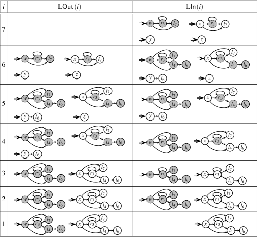
Figure 9: Liveness access graphs including implicit liveness information for the program in Figure 1. Gray nodes are nodes included by link-alias computation. Intermediate nodes are shown with dotted lines.

 

Observe that in the presence of cyclic data structures, we will get alias pairs of the form $\langle\rho,\rho\mbox{\psset{unit=28.45276pt}\begin{pspicture}(0.0pt,0.0pt)(7.68224pt,5.69055pt){\psset{linewidth=0.42679pt}\psline(0.0pt,2.84528pt)(3.5566pt,2.84528pt)(3.5566pt,0.99583pt)(7.11319pt,2.84528pt)(3.5566pt,4.6947pt)(3.5566pt,2.84528pt)}\end{pspicture}}\sigma\rangle$. If a link in the cycle is live then the link alias closure will ensure that all possible links are marked live by creating cycles in the access graphs. This may cause approximation but would be safe.

3.2 Availability and Anticipability of Access Paths

Example 3.1 shows that safety of inserting an assignment $\alpha_{x}=\mbox{\sf\em null\/}$ at a program point $p$ requires that whenever control reaches $p$, every prefix of $\mbox{\sf\em Base\/}(\rho_{x})$ has a non-null l-value. Such an access path is said to be accessible at $p$. Our use of accessibility ensures the preservation of semantics in the following sense: Consider an execution path which does not have a dereferencing exception in the unoptimized program. Then the proposed optimization will also not have any dereferencing exception in the same execution path.

3.2.1 Defining Availability and Anticipability

We define an access path $\rho_{x}$ to be accessible at $p$ if all of its prefixes are available or anticipable at $p$:

• An access path $\rho_{x}$ is available at a program point $p$, if along every path reaching $p$, there exists a program point $p^{\prime}$ such that $\mbox{\sf\em Frontier\/}(\rho_{x})$ is either dereferenced or assigned a non-null l-value at $p^{\prime}$ and is not made null between $p^{\prime}$ to $p$.

• An access path $\rho_{x}$ is anticipable at a program point $p$, if along every path starting from $p$, $\mbox{\sf\em Frontier\/}(\rho_{x})$ is dereferenced before being assigned.

Since both these properties are all paths properties, all may-link aliases of the left hand side of an assignment need to be killed. Conversely, these properties can be made more precise by including must-aliases in the set of anticipable or available paths.

Recall that comparisons in conditionals consists of simple variables only. The use of these variables does not involve any dereferencing. Hence a comparison $x==y$ does not contribute to accessibility of $x$ or $y$.

$\begin{array}[]{|@{\ }l@{\ }|@{\ }c@{\ }|@{\ }c@{\ }|@{\ }c@{\ }|}\hline\cr\mbox{Statement }s&\mbox{$Av{\mbox{\em Kill}}$}_{s}&\mbox{$Av{\mbox{\em Direct}}$}_{s}&\mbox{$Av{\mbox{\em Transfer}}$}_{s}(X)\\ \hline\cr\hline\cr\alpha_{x}=\alpha_{y}&\{\rho_{z}\mbox{\psset{unit=28.45276pt}\begin{pspicture}(0.0pt,0.0pt)(7.68224pt,5.69055pt){\psset{linewidth=0.42679pt}\psline(0.0pt,2.84528pt)(3.5566pt,2.84528pt)(3.5566pt,0.99583pt)(7.11319pt,2.84528pt)(3.5566pt,4.6947pt)(3.5566pt,2.84528pt)}\end{pspicture}}*\mid\rho_{z}\in\ \mbox{\sf LnA}(\rho_{x},\mbox{{\sf$\mathbb{A}$In}}(s))\}&(\mbox{\sf\em Base\/}(\rho_{x}))&\{\rho_{x}\mbox{\psset{unit=28.45276pt}\begin{pspicture}(0.0pt,0.0pt)(7.68224pt,5.69055pt){\psset{linewidth=0.42679pt}\psline(0.0pt,2.84528pt)(3.5566pt,2.84528pt)(3.5566pt,0.99583pt)(7.11319pt,2.84528pt)(3.5566pt,4.6947pt)(3.5566pt,2.84528pt)}\end{pspicture}}\sigma\mid\rho_{y}\mbox{\psset{unit=28.45276pt}\begin{pspicture}(0.0pt,0.0pt)(7.68224pt,5.69055pt){\psset{linewidth=0.42679pt}\psline(0.0pt,2.84528pt)(3.5566pt,2.84528pt)(3.5566pt,0.99583pt)(7.11319pt,2.84528pt)(3.5566pt,4.6947pt)(3.5566pt,2.84528pt)}\end{pspicture}}\sigma\in X\}\\ &&\cup(\mbox{\sf\em Base\/}(\rho_{y}))&\\ \hline\cr\alpha_{x}=f(\alpha_{y})&\{\rho_{z}\mbox{\psset{unit=28.45276pt}\begin{pspicture}(0.0pt,0.0pt)(7.68224pt,5.69055pt){\psset{linewidth=0.42679pt}\psline(0.0pt,2.84528pt)(3.5566pt,2.84528pt)(3.5566pt,0.99583pt)(7.11319pt,2.84528pt)(3.5566pt,4.6947pt)(3.5566pt,2.84528pt)}\end{pspicture}}*\mid\rho_{z}\in\ \mbox{\sf LnA}(\rho_{x},\mbox{{\sf$\mathbb{A}$In}}(s))\}&(\mbox{\sf\em Base\/}(\rho_{x}))&\emptyset\\ \hline\cr\alpha_{x}=\mbox{\sf\em new\/}&\{\rho_{z}\mbox{\psset{unit=28.45276pt}\begin{pspicture}(0.0pt,0.0pt)(7.68224pt,5.69055pt){\psset{linewidth=0.42679pt}\psline(0.0pt,2.84528pt)(3.5566pt,2.84528pt)(3.5566pt,0.99583pt)(7.11319pt,2.84528pt)(3.5566pt,4.6947pt)(3.5566pt,2.84528pt)}\end{pspicture}}*\mid\rho_{z}\in\ \mbox{\sf LnA}(\rho_{x},\mbox{{\sf$\mathbb{A}$In}}(s))\}&(\rho_{x})&\emptyset\\ \hline\cr\alpha_{x}=\mbox{\sf\em null\/}&\{\rho_{z}\mbox{\psset{unit=28.45276pt}\begin{pspicture}(0.0pt,0.0pt)(7.68224pt,5.69055pt){\psset{linewidth=0.42679pt}\psline(0.0pt,2.84528pt)(3.5566pt,2.84528pt)(3.5566pt,0.99583pt)(7.11319pt,2.84528pt)(3.5566pt,4.6947pt)(3.5566pt,2.84528pt)}\end{pspicture}}*\mid\rho_{z}\in\ \mbox{\sf LnA}(\rho_{x},\mbox{{\sf$\mathbb{A}$In}}(s))\}&(\mbox{\sf\em Base\/}(\rho_{x}))&\emptyset\\ \hline\cr\mbox{\sf\em use\/}\;\alpha_{y}.d&\emptyset&(\rho_{y})&\emptyset\\ \hline\cr\mbox{\sf\em return\/}\;\alpha_{y}&\emptyset&(\mbox{\sf\em Base\/}(\rho_{y}))&\emptyset\\ \hline\cr\mbox{other}&\emptyset&\emptyset&\emptyset\\ \hline\cr\end{array}$

Figure 10: Flow functions for availability. $\mbox{{\sf$\mathbb{A}$In}}(s)$ denotes the set of may-aliases at the entry of $s$.

 

Definition 3.3.

Availability. The set of paths which are available at a program point $p$, denoted by $\mbox{\em Avail\/}_{p}$, is defined as follows.

$$\mbox{\em Avail\/}_{p} = \displaystyle\bigcap_{\psi\in Paths(p)}(\mbox{\em PathAvail\/}^{\psi}_{p})$$

where, $\psi\in Paths(p)$ is a control flow path Entry to $p$ and $\mbox{\em PathAvail\/}^{\psi}_{p}$ denotes the availability at $p$ along $\psi$ and is defined as follows. If $p$ is not Entry of the procedure being analyzed, then let the statement which precedes it be denoted by $s$ and the program point immediately preceding $s$ be denoted by $p^{\prime}$. Then,

$$\mbox{\em PathAvail\/}^{\psi}_{p} = \left\{\begin{array}[]{cl}\emptyset&p\mbox{ is \mbox{\sf\em Entry\/}}\\ \mbox{\em StatementAvail\/}_{s}(\mbox{\em PathAvail\/}^{\psi}_{p^{\prime}})&\mbox{otherwise}\end{array}\right.$$

where the flow function for $s$ is defined as follows:

$$\mbox{\em StatementAvail\/}_{s}(X) = (X-\mbox{$Av{\mbox{\em Kill}}$}_{s})\;\cup\;\mbox{$Av{\mbox{\em Direct}}$}_{s}\;\cup\;\mbox{$Av{\mbox{\em Transfer}}$}_{s}(X)$$

$\mbox{$Av{\mbox{\em Kill}}$}_{s}$ denotes the sets of access paths which cease to be available after statement $s$, $\mbox{$Av{\mbox{\em Direct}}$}_{s}$ denotes the set of access paths which become available due to local effect of $s$ and $\mbox{$Av{\mbox{\em Transfer}}$}_{s}(X)$ denotes the the set of access paths which become available after $s$ due to transfer. They are defined in Figure 10. $\Box$

In a similar manner, we define anticipability of access paths.

$\begin{array}[]{|@{\ }l@{\ }|@{\ }c@{\ }|@{\ }c@{\ }|@{\ }c@{\ }|}\hline\cr\mbox{Statement }s&\mbox{$An{\mbox{\em Kill}}$}_{s}&\mbox{$An{\mbox{\em Direct}}$}_{s}&\mbox{$An{\mbox{\em Transfer}}$}_{s}(X)\\ \hline\cr\hline\cr\alpha_{x}=\alpha_{y}&\{\rho_{z}\mbox{\psset{unit=28.45276pt}\begin{pspicture}(0.0pt,0.0pt)(7.68224pt,5.69055pt){\psset{linewidth=0.42679pt}\psline(0.0pt,2.84528pt)(3.5566pt,2.84528pt)(3.5566pt,0.99583pt)(7.11319pt,2.84528pt)(3.5566pt,4.6947pt)(3.5566pt,2.84528pt)}\end{pspicture}}*\mid\rho_{z}\in\ \mbox{\sf LnA}(\rho_{x},\mbox{{\sf$\mathbb{A}$Out}}(s))\}&(\mbox{\sf\em Base\/}(\rho_{x}))&\{\rho_{y}\mbox{\psset{unit=28.45276pt}\begin{pspicture}(0.0pt,0.0pt)(7.68224pt,5.69055pt){\psset{linewidth=0.42679pt}\psline(0.0pt,2.84528pt)(3.5566pt,2.84528pt)(3.5566pt,0.99583pt)(7.11319pt,2.84528pt)(3.5566pt,4.6947pt)(3.5566pt,2.84528pt)}\end{pspicture}}\sigma\mid\rho_{x}\mbox{\psset{unit=28.45276pt}\begin{pspicture}(0.0pt,0.0pt)(7.68224pt,5.69055pt){\psset{linewidth=0.42679pt}\psline(0.0pt,2.84528pt)(3.5566pt,2.84528pt)(3.5566pt,0.99583pt)(7.11319pt,2.84528pt)(3.5566pt,4.6947pt)(3.5566pt,2.84528pt)}\end{pspicture}}\sigma\in X\}\\ &&\cup(\mbox{\sf\em Base\/}(\rho_{y}))&\\ \hline\cr\alpha_{x}=f(\alpha_{y})&\{\rho_{z}\mbox{\psset{unit=28.45276pt}\begin{pspicture}(0.0pt,0.0pt)(7.68224pt,5.69055pt){\psset{linewidth=0.42679pt}\psline(0.0pt,2.84528pt)(3.5566pt,2.84528pt)(3.5566pt,0.99583pt)(7.11319pt,2.84528pt)(3.5566pt,4.6947pt)(3.5566pt,2.84528pt)}\end{pspicture}}*\mid\rho_{z}\in\ \mbox{\sf LnA}(\rho_{x},\mbox{{\sf$\mathbb{A}$Out}}(s))\}&(\mbox{\sf\em Base\/}(\rho_{x}))&\emptyset\\ &&\cup(\mbox{\sf\em Base\/}(\rho_{y}))&\\ \hline\cr\alpha_{x}=\mbox{\sf\em new\/}&\{\rho_{z}\mbox{\psset{unit=28.45276pt}\begin{pspicture}(0.0pt,0.0pt)(7.68224pt,5.69055pt){\psset{linewidth=0.42679pt}\psline(0.0pt,2.84528pt)(3.5566pt,2.84528pt)(3.5566pt,0.99583pt)(7.11319pt,2.84528pt)(3.5566pt,4.6947pt)(3.5566pt,2.84528pt)}\end{pspicture}}*\mid\rho_{z}\in\ \mbox{\sf LnA}(\rho_{x},\mbox{{\sf$\mathbb{A}$Out}}(s))\}&(\mbox{\sf\em Base\/}(\rho_{x}))&\emptyset\\ \hline\cr\alpha_{x}=\mbox{\sf\em null\/}&\{\rho_{z}\mbox{\psset{unit=28.45276pt}\begin{pspicture}(0.0pt,0.0pt)(7.68224pt,5.69055pt){\psset{linewidth=0.42679pt}\psline(0.0pt,2.84528pt)(3.5566pt,2.84528pt)(3.5566pt,0.99583pt)(7.11319pt,2.84528pt)(3.5566pt,4.6947pt)(3.5566pt,2.84528pt)}\end{pspicture}}*\mid\rho_{z}\in\ \mbox{\sf LnA}(\rho_{x},\mbox{{\sf$\mathbb{A}$Out}}(s))\}&(\mbox{\sf\em Base\/}(\rho_{x}))&\emptyset\\ \hline\cr\mbox{\sf\em use\/}\;\alpha_{y}.d&\emptyset&(\rho_{y})&\emptyset\\ \hline\cr\mbox{\sf\em return\/}\;\alpha_{y}&\emptyset&(\mbox{\sf\em Base\/}(\rho_{y}))&\emptyset\\ \hline\cr\mbox{other}&\emptyset&\emptyset&\emptyset\\ \hline\cr\end{array}$

Figure 11: Flow functions for anticipability. $\mbox{{\sf$\mathbb{A}$Out}}(s)$ denotes the set of may-aliases at the exit of $s$.

 

Definition 3.4.

Anticipability. The set of paths which are anticipable at a program point $p$, denoted by $\mbox{\em Ant\/}_{p}$ is defined as follows.

$$\mbox{\em Ant\/}_{p} = \displaystyle\bigcap_{\psi\in Paths(p)}(\mbox{\em PathAnt\/}^{\psi}_{p})$$

where, $\psi\in Paths(p)$ is a control flow path $p$ to Exit and $\mbox{\em PathAvail\/}^{\psi}_{p}$ denotes the anticipability at $p$ along $\psi$ and is defined as follows. If $p$ is Exit then let the statement which follows it be denoted by $s$ and the program point immediately following $s$ be denoted by $p^{\prime}$. Then,

$$\mbox{\em PathAnt\/}^{\psi}_{p} = \left\{\begin{array}[]{cl}\emptyset&p\mbox{ is \mbox{\sf\em Exit\/}}\\ \ \mbox{\em StatementAnt\/}_{s}(\mbox{\em PathAnt\/}^{\psi}_{p^{\prime}})&\mbox{otherwise}\end{array}\right.$$

where the flow function for $s$ is defined as follows:

$$\mbox{\em StatementAnt\/}_{s}(X) = (X-\mbox{$An{\mbox{\em Kill}}$}_{s})\;\cup\;\mbox{$An{\mbox{\em Direct}}$}_{s}\;\cup\;\mbox{$An{\mbox{\em Transfer}}$}_{s}(X)$$

$\mbox{$An{\mbox{\em Kill}}$}_{s}$ denotes the sets of access paths which cease to be anticipable before statement $s$, $\mbox{$An{\mbox{\em Direct}}$}_{s}$ denotes the set of access paths which become anticipable due to local effect of $s$ and $\mbox{$An{\mbox{\em Transfer}}$}_{s}(X)$ denotes the the set of access paths which become anticipable before $s$ due to transfer. They are defined in Figure 11. $\Box$

Observe that both $\mbox{\em Avail\/}_{p}$ and $\mbox{\em Ant\/}_{p}$ are prefix-closed.

3.2.2 Data Flow Analyses for Availability and Anticipability

Availability and Anticipability are all (control-flow) paths properties in that the desired property must hold along every path reaching/leaving the program point under consideration. Thus these analyses identify access paths which are common to all control flow paths including acyclic control flow paths. Since acyclic control flow paths can generate only acyclic and hence finite access paths, anticipability and availability analyses deal with a finite number of access paths and summarization is not required.

Thus there is no need to use access graphs for availability and anticipability analyses. The data flow analysis can be performed using a set of access paths because the access paths are bounded and the sets would be finite. Moreover, since the access paths resulting from anticipability and availability are prefix-closed, they can be represented efficiently.

The data flow equations are same as the definitions of these analyses except that definitions are path-based (i.e. they define MoP solution) while the data flow equations are edge-based (i.e. they define MFP solution) as is customary in data flow analysis. In other words, the data flow information is merged at the intermediate points and availability and anticipability information is derived from the corresponding information at the preceding and following program point respectively. As observed in appendix A, the flow functions in availability and anticipability analyses are non-distributive hence MoP and MFP solutions may be different.

For brevity, we omit the data flow equations. We use the universal set of access paths as the initial value for all blocks other than Entry for availability analysis and Exit for anticipability analysis.

 

Figure 12: Availability and anticipability for the program in Figure 1.

Example 3.5.

Figure 12 gives the availability and anticipability information for program in Figure 1. $\mbox{{\sf$\mathbb{A}$vIn}$$}(i)$ and $\mbox{{\sf$\mathbb{A}$vOut}$$}(i)$ denote the set of available access paths before and after the statement $i$, while $\mbox{{\sf$\mathbb{A}$nIn}$$}(i)$ and $\mbox{{\sf$\mathbb{A}$nOut}$$}(i)$ denote the set of anticipable access paths before and after the statement $i$. $\Box$

4 null Assignment Insertion

We now explain how the analyses described in preceding sections can be used to insert appropriate null assignments to nullify dead links. The inserted assignments should be safe and profitable as defined below.

Definition 4.1.

Safety. It is safe to insert an assignment $\alpha=\mbox{\sf\em null\/}$ at a program point $p$ if and only if $\rho$ is not live at $p$ and $\mbox{\sf\em Base\/}(\rho)$ can be dereferenced without raising an exception.

An access path $\rho$ is nullable at a program point $p$ if and only if it is safe to insert assignment $\alpha=\mbox{\sf\em null\/}$ at $p$.

Definition 4.2.

Profitability. It is profitable to insert an assignment $\alpha=\mbox{\sf\em null\/}$ at a program point $p$ if and only if no proper prefix of $\rho$ is nullable at $p$ and the link corresponding to $\mbox{\sf\em Frontier\/}(\rho)$ is not made null before execution reaches $p$.

Note that profitability definition is strict in that every control flow path may nullify a particular link only once. Redundant null assignments on any path are prohibited. Since control flow paths have common segments, a null assignment may be partially redundant in the sense that it may be redundant along one path but not along some other path. Such null assignments will be deemed unprofitable by Definition 4.2. Our algorithm may not be able to avoid all redundant assignments.

Example 4.3.

We illustrate some situations of safety and profitability for the program in Figure 1.

• Access path $x\mbox{\psset{unit=28.45276pt}\begin{pspicture}(0.0pt,0.0pt)(7.68224pt,5.69055pt){\psset{linewidth=0.42679pt}\psline(0.0pt,2.84528pt)(3.5566pt,2.84528pt)(3.5566pt,0.99583pt)(7.11319pt,2.84528pt)(3.5566pt,4.6947pt)(3.5566pt,2.84528pt)}\end{pspicture}}\mbox{\em lptr\/}\mbox{\psset{unit=28.45276pt}\begin{pspicture}(0.0pt,0.0pt)(7.68224pt,5.69055pt){\psset{linewidth=0.42679pt}\psline(0.0pt,2.84528pt)(3.5566pt,2.84528pt)(3.5566pt,0.99583pt)(7.11319pt,2.84528pt)(3.5566pt,4.6947pt)(3.5566pt,2.84528pt)}\end{pspicture}}\mbox{\em lptr\/}$ is not nullable at the entry of 6. This is because $x\mbox{\psset{unit=28.45276pt}\begin{pspicture}(0.0pt,0.0pt)(7.68224pt,5.69055pt){\psset{linewidth=0.42679pt}\psline(0.0pt,2.84528pt)(3.5566pt,2.84528pt)(3.5566pt,0.99583pt)(7.11319pt,2.84528pt)(3.5566pt,4.6947pt)(3.5566pt,2.84528pt)}\end{pspicture}}\mbox{\em lptr\/}\mbox{\psset{unit=28.45276pt}\begin{pspicture}(0.0pt,0.0pt)(7.68224pt,5.69055pt){\psset{linewidth=0.42679pt}\psline(0.0pt,2.84528pt)(3.5566pt,2.84528pt)(3.5566pt,0.99583pt)(7.11319pt,2.84528pt)(3.5566pt,4.6947pt)(3.5566pt,2.84528pt)}\end{pspicture}}\mbox{\em lptr\/}$ is implicitly live, due to the use of $y\mbox{\psset{unit=28.45276pt}\begin{pspicture}(0.0pt,0.0pt)(7.68224pt,5.69055pt){\psset{linewidth=0.42679pt}\psline(0.0pt,2.84528pt)(3.5566pt,2.84528pt)(3.5566pt,0.99583pt)(7.11319pt,2.84528pt)(3.5566pt,4.6947pt)(3.5566pt,2.84528pt)}\end{pspicture}}\mbox{\em lptr\/}$ in 6. Hence it is not safe to insert $x.\mbox{\em lptr\/}.\mbox{\em lptr\/}=\mbox{\sf\em null\/}$ at the entry of 6.

• Access path $x\mbox{\psset{unit=28.45276pt}\begin{pspicture}(0.0pt,0.0pt)(7.68224pt,5.69055pt){\psset{linewidth=0.42679pt}\psline(0.0pt,2.84528pt)(3.5566pt,2.84528pt)(3.5566pt,0.99583pt)(7.11319pt,2.84528pt)(3.5566pt,4.6947pt)(3.5566pt,2.84528pt)}\end{pspicture}}\mbox{\em rptr\/}$ is nullable at the entry of 4, and continues to be so on the path from the entry of 4 to the entry of 7. The assignment $x.\mbox{\em rptr\/}=\mbox{\sf\em null\/}$ is profitable only at the entry of 4. $\Box$

Section 4.1 describes the criteria for deciding whether a given path $\rho$ should be considered for a null assignment at a program point $p$. Section 4.2 describes how we create the set of candidate access paths. Let Live($p$), Available($p$), and Anticipable($p$) denote set of live paths, set of available paths and set of anticipable paths respectively at program point $p$. They refer to $\mbox{{\sf$\mathbb{L}$In}$$}(i)$, $\mbox{{\sf$\mathbb{A}$vIn}$$}(i)$, and $\mbox{{\sf$\mathbb{A}$nIn}$$}(i)$ respectively when $p$ is In_i. When $p$ is Out_i, they refer to $\mbox{{\sf$\mathbb{L}$Out}$$}(i)$, $\mbox{{\sf$\mathbb{A}$vOut}$$}(i)$, and $\mbox{{\sf$\mathbb{A}$nOut}$$}(i)$ respectively.

4.1 Computing Safety and Profitability

To find out if $\rho$ can be nullified at $p$, we compute two predicates: Nullable and Nullify. $\mbox{\em Nullable}(\rho,p)$ captures the safety property—it is true if insertion of assignment $\alpha=\mbox{\sf\em null\/}$ at program point $p$ is safe.

$$\mbox{\em Nullable}(\rho,p) = \rho\not\in\mbox{{\em Live\/}($p$)}\;\wedge\;\mbox{\sf\em Base\/}(\rho)\in\mbox{{\em Available\/}($p$) $\cup$ {\em Anticipable\/}($p$)}$$ (25)

$\mbox{\em Nullify}(\rho,p)$ captures the profitability property—it is true if insertion of assignment $\alpha=\mbox{\sf\em null\/}$ at program point $p$ is profitable. To compute Nullify, we note that it is most profitable to set a link to null at the earliest point where it ceases to be live. Therefore, the Nullify  predicate at a point has to take into account the possibility of null assignment insertion at previous point(s). For a statement $i$ in the program, let In_i and Out_i denote the program points immediately before and after $i$. Then,

$$\mbox{\em Nullify}(\rho,\mbox{\sf Out${}_{i}$}) = \mbox{\em Nullable}(\rho,\mbox{\sf Out${}_{i}$})\wedge(\bigwedge_{\rho^{\prime}\in\mbox{\scriptsize\em ProperPrefix}(\rho)}\rho^{\prime}\not\in\mbox{{\em Live\/}($\mbox{\sf Out${}_{i}$}$)})$$ (26)

$$\wedge\;(\neg\mbox{\em Nullable}(\rho,\mbox{\sf In${}_{i}$})\vee\neg\mbox{\sf\em Transp\/}(\rho,i))$$

$$\mbox{\em Nullify}(\rho,\mbox{\sf In${}_{i}$}) = \mbox{\em Nullable}(\rho,\mbox{\sf In${}_{i}$})\wedge(\bigwedge_{\rho^{\prime}\in\mbox{\scriptsize\em ProperPrefix}(\rho)}\rho^{\prime}\not\in\mbox{{\em Live\/}($\mbox{\sf In${}_{i}$}$)})$$ (27)

$$\wedge\;\rho\neq\mbox{\sf\em lhs\/}(i)\wedge(\neg\!\!\!\!\bigwedge_{j\in pred(i)}\!\!\!\!\!\!\mbox{\em Nullable}(\rho,\mbox{\sf Out${}_{j}$}))$$

where, Transp($\rho$, $i$) denotes that $\rho$ is transparent with respect to statement $i$, i.e. no prefix of $\rho$ is may-link-aliased to the access path corresponding to the lhs of statement $i$ at In_i. lhs($i$) denotes the access path corresponding to the lhs access expression of assignment in statement $i$. $pred(i)$ is the set of predecessors of statement $i$ in the program. $\mbox{\em ProperPrefix}(\rho)$ is the set of all proper prefixes of $\rho$.

We insert assignment $\alpha=\mbox{\sf\em null\/}$ at program point $p$ if $\mbox{\em Nullify}(\rho,p)$ is true.

4.2 Computing Candidate Access Paths for null Insertion

The method described above only checks whether a given access path $\rho$ can be nullified at a given program point $p$. We can generate the candidate set of access paths for null insertion at $p$ as follows: For any candidate access path $\rho$, $\mbox{\sf\em Base\/}(\rho)$ must either be available or anticipable at $p$. Additionally, all simple access paths are also candidates for null insertions. Therefore,

$$\mbox{\em Candidates}(p) = \left\{\rho\mbox{\psset{unit=28.45276pt}\begin{pspicture}(0.0pt,0.0pt)(7.68224pt,5.69055pt){\psset{linewidth=0.42679pt}\psline(0.0pt,2.84528pt)(3.5566pt,2.84528pt)(3.5566pt,0.99583pt)(7.11319pt,2.84528pt)(3.5566pt,4.6947pt)(3.5566pt,2.84528pt)}\end{pspicture}}f\mid\rho\in\mbox{{\em Available\/}($p$) $\cup$ {\em Anticipable\/}($p$)},f\in\mbox{\em OutField}(\rho)\right\}$$ (28)

$$\cup\left\{\rho\mid\rho\mbox{ is a simple access path }\right\}$$

Where $\mbox{\em OutField}(\rho)$ is the set of fields which can be used to extend access path $\rho$ at $p$. It can be obtained easily from the type information of the object $\mbox{\sf\em Target\/}(\rho)$ at $p$.

Figure 13: Null insertion for the program in Figure 1.

 

Note that all the information required for equations (25), (26), (27), and (28) is obtained from the result of data flow analyses described in preceding sections. Type information of objects required by equation (28) can be obtained from the front end of compiler. Transp uses may alias information as computed in terms of pairs of access graph.

Example 4.4.

Figure 13 lists a trace of the null insertion algorithm for the program in Figure 1. $\Box$

4.3 Reducing Redundant null Insertions

Consider a program with an assignment statement $i:\alpha_{x}=\alpha_{y}$. Assume a situation where, for some non-empty suffix $\sigma$, both $\mbox{\em Nullify}(\rho_{y}\mbox{\psset{unit=28.45276pt}\begin{pspicture}(0.0pt,0.0pt)(7.68224pt,5.69055pt){\psset{linewidth=0.42679pt}\psline(0.0pt,2.84528pt)(3.5566pt,2.84528pt)(3.5566pt,0.99583pt)(7.11319pt,2.84528pt)(3.5566pt,4.6947pt)(3.5566pt,2.84528pt)}\end{pspicture}}\sigma,\mbox{\sf In${}_{i}$})$ and $\mbox{\em Nullify}(\rho_{x}\mbox{\psset{unit=28.45276pt}\begin{pspicture}(0.0pt,0.0pt)(7.68224pt,5.69055pt){\psset{linewidth=0.42679pt}\psline(0.0pt,2.84528pt)(3.5566pt,2.84528pt)(3.5566pt,0.99583pt)(7.11319pt,2.84528pt)(3.5566pt,4.6947pt)(3.5566pt,2.84528pt)}\end{pspicture}}\sigma,\mbox{\sf Out${}_{i}$})$ are true. In that case, we will be inserting $\alpha_{y}.\sigma=\mbox{\sf\em null\/}$ at In_i and $\alpha_{x}.\sigma=\mbox{\sf\em null\/}$ at Out_i. Clearly, the latter null assignment is redundant in this case and can be avoided by checking if $\rho_{y}\mbox{\psset{unit=28.45276pt}\begin{pspicture}(0.0pt,0.0pt)(7.68224pt,5.69055pt){\psset{linewidth=0.42679pt}\psline(0.0pt,2.84528pt)(3.5566pt,2.84528pt)(3.5566pt,0.99583pt)(7.11319pt,2.84528pt)(3.5566pt,4.6947pt)(3.5566pt,2.84528pt)}\end{pspicture}}\sigma$ is nullable at In_i.

If must-alias analysis is performed then redundant assignments can be reduced further. Since must-link-alias relation is symmetric, reflexive, and transitive and hence an equivalence relation, the set of candidate paths at a program point can be divided into equivalence classes based on must-link-alias relation. Redundant null assignments can be reduced by nullifying at most one access path in any equivalence class.

5 Convergence of Heap Reference Analysis

The null assignment insertion algorithm makes a single traversal over the control flow graph. We show the termination of liveness analysis using the properties of access graph operations. Termination of availability and anticipability can be shown by similar arguments over finite sets of bounded access paths. Termination of alias analysis follows from hind99interprocedural.

5.1 Monotonicity

For a program there are a finite number of basic blocks, a finite number of fields for any root variable, and a finite number of field names in any access expression. Hence the number of access graphs for a program is finite. Further, the number of nodes and hence the size of each access graph, is bounded by the number of labels which can be created for a program.

Access graphs for a variable $x$ form a complete lattice with a partial order $\sqsubseteq_{G}$ induced by ${\;\uplus\;}$. Note that ${\;\uplus\;}$ is commutative, idempotent, and associative. Let $G=\langle x,N_{F},N_{I},E\rangle$ and $G^{\prime}=\langle x,N^{\prime}_{F},N^{\prime}_{I},E^{\prime}\rangle$ where subscripts $F$ and $I$ distinguish between the final and intermediate nodes. The partial order $\sqsubseteq_{G}$ is defined as

$$G\sqsubseteq_{G}G^{\prime}\Leftrightarrow\left(N^{\prime}_{F}\subseteq N_{F}\right)\wedge\left(N^{\prime}_{I}\subseteq\left(N_{F}\cup N_{I}\right)\right)\wedge\left(E^{\prime}\subseteq E\right)$$

Clearly, $G\sqsubseteq_{G}G^{\prime}$ implies that $G$ contains all access paths of $G^{\prime}$. We extend $\sqsubseteq_{G}$ to a set of access graphs as follows:

$$S_{1}\sqsubseteq_{S}S_{2}\Leftrightarrow\forall G_{2}\in S_{2},\exists G_{1}\in S_{1}\mbox{ s.t. }G_{1}\sqsubseteq_{G}G_{2}$$

It is easy to verify that $\sqsubseteq_{G}$ is reflexive, transitive, and antisymmetric. For a given variable $x$, the access graph $\mbox{$\mathcal{E}$}\!_{G}$ forms the $\top$ element of the lattice while the $\bot$ element is a greatest lower bound of all access graphs.

The partial order over access graphs and their sets can be carried over unaltered to remainder graphs ($\sqsubseteq_{RG}$) and their sets ($\sqsubseteq_{RS}$), with the added condition that ${$\epsilon$}_{RG}$ is incomparable to any other non empty remainder graph.

Operation	Monotonicity
Union	$G_{1}\sqsubseteq_{G}G_{1}^{\prime}\wedge G_{2}\sqsubseteq_{G}G_{2}^{\prime}$	$\Rightarrow$	$G_{1}{\;\uplus\;}G_{2}\sqsubseteq_{G}G_{1}^{\prime}{\;\uplus\;}G_{2}^{\prime}$
Path Removal	$G_{1}\sqsubseteq_{G}G_{2}$	$\Rightarrow$	$G_{1}\ominus\rho\sqsubseteq_{G}G_{2}\ominus\rho$
Factorization	$G_{1}\sqsubseteq_{G}G_{2}$	$\Rightarrow$	$G_{1}/(G,M)\sqsubseteq_{RS}G_{2}/(G,M)$
Extension	$RS_{1}\sqsubseteq_{RS}RS_{2}\wedge G_{1}\sqsubseteq_{G}G_{2}\wedge M_{1}\subseteq M_{2}$	$\Rightarrow$	$\mbox{$(G_{1},M_{1})\#\,RS_{1}$}\sqsubseteq_{G}\mbox{$(G_{2},M_{2})\#\,RS_{2}$}$
Link-Alias Closure	$G_{1}\sqsubseteq_{G}G^{\prime}_{1}\wedge G_{2}\sqsubseteq_{G}G^{\prime}_{2}$	$\Rightarrow$	$\mbox{\sf LnG}(G_{1},G_{2},\langle g_{x},g_{y}\rangle)\sqsubseteq_{S}\mbox{\sf LnG}(G^{\prime}_{1},G^{\prime}_{2},\langle g_{x},g_{y}\rangle)$

Figure 14: Monotonicity of Access Graph Operations

  .

Access graph operations are monotonic as described in Figure 14. Path removal is monotonic in the first argument but not in the second argument. Similarly factorization is monotonic in the first argument but not in the second and the third argument. However, we show that in each context where they are used, the resulting functions are monotonic:

1. Path removal is used only for an assignment $\alpha_{x}=\alpha_{y}$. It is used in liveness analysis and its second argument is $\rho_{x}$ which is constant for any assignment statement $\alpha_{x}=\alpha_{y}$. Thus the resulting flow functions are monotonic.

2. Factorization is used in the following situations:

   1. Link-alias closure of access graphs. From equation (21) it is clear LnG is monotonic in the first argument (because it is used in ${\;\uplus\;}$) and the second argument (because it is supplied as the first argument of factorization). The third and the fourth arguments of LnG are linear access graphs containing a single path and hence are incomparable with any other linear access graph. Thus link-alias computation is monotonic in all its arguments.

   2. Liveness analysis. Factorization is used for the flow function corresponding to an assignment $\alpha_{x}=\alpha_{y}$ and its second argument is G$({\rho_{x}})$ while its third argument is lastNode$({\mbox{{\sf\em\small G\/}$({\rho_{x}})$}})$ both of which are constant for any assignment statement $\alpha_{x}=\alpha_{y}$. Thus, the resulting flow functions are monotonic.

Thus we conclude that all flow functions are monotonic. Since lattices are finite, termination of heap reference analysis follows.

Appendix A discusses the distributivity of flow functions.

5.2 Complexity

This section discusses the issues which influence the complexity and efficiency of performing heap reference analysis. Empirical measurements which corroborate the observations made in this section are presented in Section 7.

The data flow frameworks defined in this paper are not separable [Khedker (2002)] because the data flow information of a variable depends on the data flow information of other variables. Thus the number of iterations over control flow graph is not bounded by the depth of the graph [Aho et al. (1986), Hecht (1977), Khedker (2002)] but would also depend on the number of root variables which depend on each other.

Although we consider each statement to be a basic block, our control flow graphs retain only statements involving references. A further reduction in the size of control flow graphs follows from the fact that successive use statements need not be kept separate and can be grouped together into a block which ends on a reference assignment.

The amount of work done in each iteration is not fixed but depends on the size of access graphs. Of all operations performed in an iteration, only CFN$({G},{G^{\prime}})$ is costly. Conversion to deterministic access graphs is also a costly operations but is performed for a single pass during null assignment insertion. In practice, the access graphs are quite small because of the following reason: Recall that edges in access graphs capture dependence of a reference made at one program point on some other reference made at another point (Section 2.4.1). In real programs, traversals involving long dependences are performed using iterative constructs in the program. In such situations, the length of the chain of dependences is limited by the process of summarization because summarization treats nodes with the same label as being identical. Thus, in real programs chains of such dependences, and hence the access graphs, are quite small in size. This is corroborated by Figure 16 which provides the empirical data for the access graphs in our examples. The average number of nodes in these access graphs is less than 7 while the average number of edges is less than 12. These numbers are still smaller in the interprocedural analysis. Hence the complexities of access graph operations is not a matter of concern.

6 Safety of null Assignment Insertion

We have to prove that the null assignments inserted by our algorithm (Section 4) in a program are safe in that they do not alter the result of executing the program. We do this by showing that (a) an inserted statement itself does not raise a dereferencing exception, and (b) an inserted statement does not affect any other statement, both original and inserted.

We use the subscripts $b$ and $a$ for a program point $p$ to denote “before” and “after” in an execution order. Further, the corresponding program points in the original and modified program are distinguished by the superscript $o$ and $m$. The correspondence is defined as follows: If $p^{m}$ is immediately before or after an inserted assignment $\alpha=\mbox{\sf\em null\/}$, $p^{o}$ is the point where the decision to insert the null assignment is taken. For any other $p^{m}$, there is an obvious $p^{o}$.

We first assert the soundness of availability, anticipability and alias analyses without proving them.

Lemma 6.1.

(Soundness of Availability Analysis). Let $AV_{\!\!\mbox{$p_{a}$}}$ be the set of access paths available at program point $p_{a}$. Let $\rho\in AV_{\!\!\mbox{$p_{a}$}}$. Then along every path reaching $p_{a}$, there exists a program point $p_{b}$, such that the link represented by $\mbox{\sf\em Frontier\/}(\rho)$ is either dereferenced or assigned a non-null l-value at $p_{b}$ and is not made null between $p_{b}$ and $p_{a}$.

Lemma 6.2.

(Soundness of Anticipability Analysis). Let $AN_{p}$ be the set of access paths anticipable at program point $p$. Let $\rho\in AN_{p}$. Then along every path starting from $p$, the link represented by $\mbox{\sf\em Frontier\/}(\rho)$ is dereferenced before being assigned.

For semantically valid input programs (i.e.  programs which do not generate dereferencing exceptions), Lemma 6.1 and Lemma 6.2 guarantee that if $\rho$ is available or anticipable at $p$, $\mbox{\sf\em Target\/}(\rho)$ can be dereferenced at $p$.

Lemma 6.3.

(Soundness of Alias Analysis). Let $\mbox{\sf\em Frontier\/}(\rho_{x})$ represents the same link as $\mbox{\sf\em Frontier\/}(\rho_{y})$ at a program point $p$ during some execution of the program. Then link-alias computation of $\rho_{x}$ at $p$ would discover $\rho_{y}$ to be link-aliased to $\rho_{x}$.

For the main claim, we relate the access paths at $p_{a}$ to the access paths at $p_{b}$ by incorporating the effect of intervening statements only, regardless of the statements executed before $p_{b}$. In some execution of a program, let $\rho$ be the access path of interest at $p_{a}$ and the sequence of statements between $p_{b}$ and $p_{a}$ be $s$. Then $T(s,\rho)$ represents the access path at $p_{b}$ which, if non-$\mathcal{E}$, can be used to access the link represented by $\mbox{\sf\em Frontier\/}(\rho)$. $T(s,\rho)$ captures the transitive effect of backward transfers of $\rho$ through $s$. $T$ is defined as follows:

$$T(s,\rho) = \left\{\begin{array}[]{ll}\rho&s\mbox{ is a use statement }\\ \rho&s\mbox{ is }\alpha_{x}=\ldots\mbox{ and }\rho_{x}\mbox{ is not a prefix of }\rho\\ \mbox{$\mathcal{E}$}&s\mbox{ is }\alpha_{x}=\mbox{{\em New\/} and }\rho=\rho_{x}\mbox{\psset{unit=28.45276pt}\begin{pspicture}(0.0pt,0.0pt)(7.68224pt,5.69055pt){\psset{linewidth=0.42679pt}\psline(0.0pt,2.84528pt)(3.5566pt,2.84528pt)(3.5566pt,0.99583pt)(7.11319pt,2.84528pt)(3.5566pt,4.6947pt)(3.5566pt,2.84528pt)}\end{pspicture}}\sigma\\ \mbox{$\mathcal{E}$}&s\mbox{ is }\alpha_{x}=\mbox{\sf\em null\/}\ \mbox{ and }\rho=\rho_{x}\mbox{\psset{unit=28.45276pt}\begin{pspicture}(0.0pt,0.0pt)(7.68224pt,5.69055pt){\psset{linewidth=0.42679pt}\psline(0.0pt,2.84528pt)(3.5566pt,2.84528pt)(3.5566pt,0.99583pt)(7.11319pt,2.84528pt)(3.5566pt,4.6947pt)(3.5566pt,2.84528pt)}\end{pspicture}}\sigma\\ \rho_{y}\mbox{\psset{unit=28.45276pt}\begin{pspicture}(0.0pt,0.0pt)(7.68224pt,5.69055pt){\psset{linewidth=0.42679pt}\psline(0.0pt,2.84528pt)(3.5566pt,2.84528pt)(3.5566pt,0.99583pt)(7.11319pt,2.84528pt)(3.5566pt,4.6947pt)(3.5566pt,2.84528pt)}\end{pspicture}}\sigma&s\mbox{ is }\alpha_{x}=\alpha_{y}\mbox{ and }\rho=\rho_{x}\mbox{\psset{unit=28.45276pt}\begin{pspicture}(0.0pt,0.0pt)(7.68224pt,5.69055pt){\psset{linewidth=0.42679pt}\psline(0.0pt,2.84528pt)(3.5566pt,2.84528pt)(3.5566pt,0.99583pt)(7.11319pt,2.84528pt)(3.5566pt,4.6947pt)(3.5566pt,2.84528pt)}\end{pspicture}}\sigma\\ \rho&s\mbox{ is the function call }\alpha_{x}=f(\alpha_{y})\mbox{ and }\\ &\mbox{\sf\em Root\/}(\rho)\mbox{ is a global variable}\\ \rho_{y}\mbox{\psset{unit=28.45276pt}\begin{pspicture}(0.0pt,0.0pt)(7.68224pt,5.69055pt){\psset{linewidth=0.42679pt}\psline(0.0pt,2.84528pt)(3.5566pt,2.84528pt)(3.5566pt,0.99583pt)(7.11319pt,2.84528pt)(3.5566pt,4.6947pt)(3.5566pt,2.84528pt)}\end{pspicture}}\sigma&s\mbox{ is the function call }\alpha_{x}=f(\alpha_{y}),\rho=z\mbox{\psset{unit=28.45276pt}\begin{pspicture}(0.0pt,0.0pt)(7.68224pt,5.69055pt){\psset{linewidth=0.42679pt}\psline(0.0pt,2.84528pt)(3.5566pt,2.84528pt)(3.5566pt,0.99583pt)(7.11319pt,2.84528pt)(3.5566pt,4.6947pt)(3.5566pt,2.84528pt)}\end{pspicture}}\sigma\mbox{ and }\\ &z\mbox{ is the formal parameter of }f\\ \rho&s\mbox{ is the return statement }return(\alpha_{z})\mbox{ and }\\ &\mbox{\sf\em Root\/}(\rho)\mbox{ is a global variable}\\ \rho_{z}\mbox{\psset{unit=28.45276pt}\begin{pspicture}(0.0pt,0.0pt)(7.68224pt,5.69055pt){\psset{linewidth=0.42679pt}\psline(0.0pt,2.84528pt)(3.5566pt,2.84528pt)(3.5566pt,0.99583pt)(7.11319pt,2.84528pt)(3.5566pt,4.6947pt)(3.5566pt,2.84528pt)}\end{pspicture}}\sigma&s\mbox{ is the return statement }return(\alpha_{z}),\rho=\rho_{x}\mbox{\psset{unit=28.45276pt}\begin{pspicture}(0.0pt,0.0pt)(7.68224pt,5.69055pt){\psset{linewidth=0.42679pt}\psline(0.0pt,2.84528pt)(3.5566pt,2.84528pt)(3.5566pt,0.99583pt)(7.11319pt,2.84528pt)(3.5566pt,4.6947pt)(3.5566pt,2.84528pt)}\end{pspicture}}\sigma\mbox{ and}\\ &\mbox{the corresponding call is }\alpha_{x}=f(\alpha_{y})\\ T(s_{1},T(s_{2},\rho))&s\mbox{ is a sequence }s_{1};s_{2}\end{array}\right.$$

Lemma 6.4.

(Liveness Propagation). Let $\rho^{a}$ be in some explicit liveness graph at $p_{a}$. Let the sequence of statements between $p_{b}$ to $p_{a}$ be $s$. Then, if $T(s,\rho^{a})=\rho^{b}$ and $\rho^{b}$ is not $\mathcal{E}$, then $\rho^{b}$ is in some explicit liveness graph at $p_{b}$.

Proof 6.5.

The proof is by structural induction on $s$. Since $\rho^{b}$ is non-$\mathcal{E}$, the base cases are:

1. $s$ is a use statement. In this case $\rho^{b}=\rho^{a}$.

2. $s$ is an assignment $\alpha_{x}=\ldots$ such that $\rho_{x}$ is not a prefix of $\rho^{a}$. Here also $\rho^{b}=\rho^{a}$.

3. $s$ is an assignment $\alpha_{x}=\alpha_{y}$ such that $\rho^{a}=\rho_{x}\mbox{\psset{unit=28.45276pt}\begin{pspicture}(0.0pt,0.0pt)(7.68224pt,5.69055pt){\psset{linewidth=0.42679pt}\psline(0.0pt,2.84528pt)(3.5566pt,2.84528pt)(3.5566pt,0.99583pt)(7.11319pt,2.84528pt)(3.5566pt,4.6947pt)(3.5566pt,2.84528pt)}\end{pspicture}}\sigma$. In this case $\rho^{b}=\rho_{y}\mbox{\psset{unit=28.45276pt}\begin{pspicture}(0.0pt,0.0pt)(7.68224pt,5.69055pt){\psset{linewidth=0.42679pt}\psline(0.0pt,2.84528pt)(3.5566pt,2.84528pt)(3.5566pt,0.99583pt)(7.11319pt,2.84528pt)(3.5566pt,4.6947pt)(3.5566pt,2.84528pt)}\end{pspicture}}\sigma$.

4. $s$ is the function call $\alpha_{x}=f(\alpha_{y})$. The only interesting case is when $\rho^{a}=z\mbox{\psset{unit=28.45276pt}\begin{pspicture}(0.0pt,0.0pt)(7.68224pt,5.69055pt){\psset{linewidth=0.42679pt}\psline(0.0pt,2.84528pt)(3.5566pt,2.84528pt)(3.5566pt,0.99583pt)(7.11319pt,2.84528pt)(3.5566pt,4.6947pt)(3.5566pt,2.84528pt)}\end{pspicture}}\sigma$, where $z$ is the formal parameter of $f$. In this case, $\rho^{b}=\rho_{y}\mbox{\psset{unit=28.45276pt}\begin{pspicture}(0.0pt,0.0pt)(7.68224pt,5.69055pt){\psset{linewidth=0.42679pt}\psline(0.0pt,2.84528pt)(3.5566pt,2.84528pt)(3.5566pt,0.99583pt)(7.11319pt,2.84528pt)(3.5566pt,4.6947pt)(3.5566pt,2.84528pt)}\end{pspicture}}\sigma$.

5. $s$ is the return statement $return(\alpha_{z})$. The only interesting case is when $\rho^{a}=\rho_{x}\mbox{\psset{unit=28.45276pt}\begin{pspicture}(0.0pt,0.0pt)(7.68224pt,5.69055pt){\psset{linewidth=0.42679pt}\psline(0.0pt,2.84528pt)(3.5566pt,2.84528pt)(3.5566pt,0.99583pt)(7.11319pt,2.84528pt)(3.5566pt,4.6947pt)(3.5566pt,2.84528pt)}\end{pspicture}}\sigma$, and the corresponding call is $\alpha_{x}=f(\alpha_{y})$. In this case, $\rho^{b}=\rho_{z}\mbox{\psset{unit=28.45276pt}\begin{pspicture}(0.0pt,0.0pt)(7.68224pt,5.69055pt){\psset{linewidth=0.42679pt}\psline(0.0pt,2.84528pt)(3.5566pt,2.84528pt)(3.5566pt,0.99583pt)(7.11319pt,2.84528pt)(3.5566pt,4.6947pt)(3.5566pt,2.84528pt)}\end{pspicture}}\sigma$.

For (1) and (2), since $\rho^{a}$ is not in E$\mathbb{L}$KillPath, $\rho^{b}$ is in some explicit liveness graph at $p_{b}$. For (3), from Equation (18), $\rho^{b}$ is in some explicit liveness graph at $p_{b}$. For (4) and (5), the result follows from the fact that $\mbox{\em Summary\/}(\rho_{y})$ and $\mbox{\em Summary\/}(\rho_{z})$ are in the explicit liveness graph of the program points before the call and return statements respectively.

For the inductive step, assume that the lemma holds for $s_{1}$ and $s_{2}$. From the definition of $T$, there exists a non-$\mathcal{E}$ $\rho^{i}$ at the intermediate point $p_{i}$ between $s_{1}$ and $s_{2}$, such that $\rho^{i}=T(s_{2},\rho^{a})$ and $\rho^{b}=T(s_{1},\rho^{i})$. Since $\rho^{a}$ is in some explicit liveness graph at $p_{a}$, by the induction hypothesis, $\rho^{i}$ must be in some explicit liveness graph at $p_{i}$. Further, by the induction hypothesis, $\rho^{b}$ must be in some explicit liveness graph at $p_{b}$.

Lemma 6.6.

Every access path which is in some liveness graph at $p^{m}_{b}$ is also in some liveness graph at $p^{o}_{b}$.

Proof 6.7.

If an extra explicitly live access path is introduced in the modified program, it could be only because of an inserted assignment $\alpha=\mbox{\sf\em null\/}$ at some $p^{m}_{a}$. The only access paths which this statement can add to an explicit liveness graph are the paths corresponding the proper prefixes of $\alpha$. However, the algorithm selects $\alpha$ for nullification only if the access paths corresponding to all its proper prefixes are in some explicit liveness graph. Therefore every access path which is in some explicit liveness graph at $p^{m}_{a}$ is also in some explicit liveness graph at $p^{o}_{a}$. The same relation would hold at $p^{m}_{b}$ and $p^{o}_{b}$.

If an extra live access path is introduced in the modified program, it could be only because of an inserted assignment $\alpha=\mbox{\sf\em null\/}$ at some $p^{m}_{a}$. The only access paths which this statement can add to an liveness graphs are $\mbox{\sf LnA}(\rho^{\prime},\mbox{\sf\em AS\/}^{m})$, where $\rho^{\prime}$ is a proper prefix of $\rho$ and $\mbox{\sf\em AS\/}^{m}$ represents the alias set at $p^{m}_{a}$. However, the algorithm selects $\alpha$ for nullification at $p^{m}_{a}$  only if the access paths corresponding to all its proper prefixes are in some liveness graph at $p^{o}_{a}$. As liveness graphs are closed under link aliasing, this implies that the liveness graph at $p^{o}_{a}$ includes paths $\mbox{\sf LnA}(\rho^{\prime},\mbox{\sf\em AS\/}^{o})$, where $\mbox{\sf\em AS\/}^{o}$ represents the alias set at $p^{o}_{a}$. Since inserted statements can only kill aliases, $\mbox{\sf\em AS\/}^{m}\subseteq\mbox{\sf\em AS\/}^{o}$. Thus, $\mbox{\sf LnA}(\rho^{\prime},\mbox{\sf\em AS\/}^{m})$, the paths resulting out of insertion, are also in the liveness graph at $p^{o}_{a}$. Therefore every access path which is in some liveness graph at $p^{m}_{a}$ is also in some liveness graph at $p^{o}_{a}$. The same relation would hold at $p^{m}_{b}$ and $p^{o}_{b}$.

Theorem 6.8.

(Safety of null insertion). Let the assignment $\alpha^{b}=\mbox{\sf\em null\/}$ be inserted by the algorithm immediately before $p^{m}_{b}$. Then:

1. Execution of $\alpha^{b}=\mbox{\sf\em null\/}$ does not raise any exception due to dereferencing.

2. Let $\alpha^{a}$ be used immediately after $p^{m}_{a}$ (in an original statement or an inserted null assignment). Then, execution of $\alpha^{b}=\mbox{\sf\em null\/}$ cannot nullify any link used in $\alpha^{a}$.

Proof 6.9.

We prove the two parts separately.

1. If $\alpha^{b}$ is a root variable, then the execution of $\alpha^{b}=\mbox{\sf\em null\/}$ cannot raise an exception. When $\alpha^{b}$ is not a root variable, from the null assignment algorithm, every proper prefix $\rho^{\prime}$ of $\rho^{b}$ is either anticipable or available. From the soundness of both these analyses, $\mbox{\sf\em Target\/}(\rho^{\prime})$ exists and the execution of $\alpha^{b}=\mbox{\sf\em null\/}$ cannot raise an exception.

2. We prove this by contradiction. Let $s$ denote the sequence of statements between $p^{m}_{b}$ and $p^{m}_{a}$. Assume that $\alpha^{b}=\mbox{\sf\em null\/}$ nullifies a link used in $\alpha^{a}$. This is possible only if there exists a prefix $\rho^{\prime}$ of $\rho^{a}$ such that $T(s,\rho^{\prime})$ shares its frontier with $\rho^{b}$ at $p^{m}_{b}$. By Lemma 6.4, $T(s,\rho^{\prime})$ must be in some explicit liveness graph at $p^{m}_{b}$. From Lemma 6.3 and the definition of liveness, $\rho^{b}$ is in some liveness graph at $p^{m}_{b}$. By Lemma 6.6, $\rho^{b}$ is also in some liveness graph at $p^{o}_{b}$. Thus a decision to insert $\alpha^{b}=\mbox{\sf\em null\/}$ cannot be taken at $p^{o}_{b}$.

7 Empirical Measurements

X axis indicates measurement instants in milliseconds. Y axis indicates heap usage in KB. Solid line represents memory required for original program while dashed line represents memory for the modified program. Observe that the modified program executed faster than the original program in each case.  

Figure 15: Temporal plots of memory usages.

In order to show the effectiveness of heap reference analysis, we have developed proof-of-concept implementations of heap reference analysis at two levels: One at the interprocedural level and the other at the intraprocedural level.

7.1 Experimentation Methodology

Our intraprocedural analyzer, which predates the interprocedural version is an evidence of the effectiveness of intraprocedural analysis. It was implemented using XSB-Prolog. The measurements were made on a 800 MHz Pentium III machine with 128 MB memory running Fedora Core release 2. The benchmarks used were Loop, DLoop, CReverse, BiSort, TreeAdd and GCBench. Three of these (Loop, DLoop and CReverse) are similar to those in [Shaham et al. (2003)]. Loop creates a singly linked list and traverses it, DLoop is doubly linked list variation of the same program, CReverse reverses a singly linked list. BiSort and TreeAdd are taken from Java version of Olden benchmark suite [Carlisle (1996)]. GCBench is taken from [(5)].

For measurements on this implementation, the function of interest in a given Java program was manually translated to Prolog representation. This allowed us to avoid redundant information like temporaries, empty statements etc. resulting in a compact representations of programs. The interprocedural information for this function was approximated in the Prolog representations in the following manner: Calls to non-recursive functions were inlined and calls to recursive functions were replaced by iterative constructs which approximated the liveness property of heap manipulations in the function bodies. The result of the analysis was used to manually insert null assignments in the original Java programs to create modified Java programs.

Manual interventions allowed us to handle procedure calls without performing interprocedural analysis. In order to automate the analysis and extend it to interprocedural level, we used SOOT [Vallée-Rai et al. (1999)] which has built in support for many of our requirements. However, compared to the Prolog representation of programs, the default Jimple representation used by SOOT is not efficient for our purposes because it introduces a large number of temporaries and contains all statements even if they do not affect heap reference analysis.

As was described earlier, our interprocedural analysis is very simplistic. Our experience shows that imprecision of interprocedural alias analysis increases the size of alias information thereby making the analysis inefficient apart from reducing the precision of the resulting information. This effect has been worsened by the fact that SOOT introduces a large number of temporary variables. Besides, the complete alias information is not required for our purposes.

We believe that our approach can be made much more scalable by

• Devising a method of avoiding full alias analysis and computing only the required alias information, and

• Improving the Jimple representation by eliminating redundant information, combining multiple successive uses into a single statement etc.

The implementations, along with the test programs (with their original, modified, and Prolog versions) are available at [Karkare (2005)].

Intraprocedural analysis of selected method (Prolog Implementation)
Program Analysis Access Graphs Execution Name.Function Time Nodes Edges Time (sec) #Iter (sec) #G Avg Max Avg Max #null Orig. Mod. Loop.main 5 0.082 172 1.13 2 0.78 2 9 1.503 1.388 DLoop.main 5 1.290 332 2.74 4 5.80 10 11 1.594 1.470 CReverse.main 5 0.199 242 1.41 4 1.10 6 8 1.512 1.414 BiSort.main 6 0.083 63 2.16 3 3.81 6 5 3.664 3.646 TreeAdd.addtree 6 0.255 132 2.84 7 4.87 14 7 1.976 1.772 GCBench.Populate 6 0.247 136 2.73 7 4.63 14 7 132.99 88.86
Interprocedural analysis of all methods (SOOT Implementation)
Program LOC # Analysis Access Graph Stats Execution Name in methods Time Nodes Edges #null Time (sec) Jimple (sec.) Max Avg Max Avg Orig. Mod. Loop 83 2 0.558 2 1.24 2 0.39 12 1.868 1.711 DLoop 78 2 20.660 5 1.45 12 0.76 12 1.898 1.772 CReverse 85 2 1.833 3 1.39 4 0.51 12 1.930 1.929 BiSort 466 12 1.498 7 1.29 10 0.40 77 1.519 1.524 TreeAdd 228 4 0.797 6 1.29 7 0.46 34 2.704 2.716 GCBench 226 9 1.447 4 1.13 5 0.16 56 122.731 60.372

• #Iter is the maximum number of iterations taken by any analysis.

• Analysis Time is the total time taken by all analyses.

• #G is total number of access graphs created by alias analysis and liveness analysis. Prolog implementation performs alias analysis also using access graphs.

• Max nodes (edges) is the maximum over number of nodes (edges) in all access graphs. In some cases, maximum number nodes/edges is more in case of intraprocedural analysis due to presence of longer paths in explicitly supplied boundary information, which gets replaced by a single * node in interprocedural analysis.

• Avg nodes (edges) is the average number of nodes (edges) over all access graphs.

• #null is the number of inserted null assignments.

Figure 16: Empirical measurements of proof-of-concept implementations of heap reference analyzer.

 

7.2 Measurements and Observations

Our experiments were directed at measuring:

1. The efficiency of analysis. We measured the total time required, number of iterations of round robin analyses, and the number and sizes of access graphs.

2. The effectiveness of null assignment insertions. The programs were made to create huge data structures. Memory usage was measured by explicit calls to garbage collector in both modified and original Java programs at specific probing points such as call sites, call returns, loop begins and loop ends. The overall execution time for the original and the modified programs was also measured.

The results of our experiments are shown in Figure 15 and Figure 16. As can be seen from Figure 15, nullification of links helped the garbage collector to collect a lot more garbage, thereby reducing the allocated heap memory. In case of BiSort, however, the links were last used within a recursive procedure which was called multiple times. Hence, safety criteria prevented null assignment insertion within the called procedure. Our analysis could only nullify the root of the data structure at the end of the program. Thus the memory was released only at the end of the program.

For interprocedural analysis, class files for both original as well as modified programs were generated using SOOT. As can be seen from Figure 16, modified programs executed faster. In general, a reduction in execution time can be attributed to the following two factors: (a) a decrease in the number of calls to garbage collector and (b) reduction in the time taken for garbage collection in each call. The former is possible because of availability of a larger amount of free memory, the latter is possible because lesser reachable memory needs to be copied. In our experiments, factor (a) above was absent because the number of (explicit) calls to garbage collector were kept same. GCBench showed a large improvement in execution time after null assignment insertion. This is because GCBench creates large trees in heap, which are not used in the program after creation and our implementation was able to nullify left and right subtrees of these trees immediately after their creation. This also reduced the high water mark of the heap memory requirement.

As explained in Section 5.2, sizes of the access graphs (average number of nodes and edges) is small. This can be verified from Figure 16. The analysis of DLoop creates a large number of access graphs because of the presence of cycles in heap. In such a case, a large number of alias pairs are generated, many of which are redundant. Though it is possible to reduce analysis time by eliminating redundant alias pairs, our implementation, being a proof-of-concept implementation, does not do so for sake of simplicity.

Our technique and implementation compares well with the technique and results described in [Shaham et al. (2003)]. A conceptual comparison with this method is included in Section 9.2. The implementation described in [Shaham et al. (2003)] runs on a 900 MHz P-III with 512 MB RAM running Windows 2000. It takes 1.76 seconds, 2.68 seconds and 4.79 seconds respectively for Loop, DLoop and CReverse for null assignment insertion. Time required by our implementation for the above mentioned programs is given in Figure 16. Our implementation automatically computes the program points for null insertion whereas their method cannot do so. Our implementation performs much better in all cases.

8 Extensions for C++

This approach becomes applicable to C++ by extending the concept of access graphs to faithfully represent the C++ memory model. It is assumed that the memory which becomes unreachable due to nullification of pointers is reclaimed by an independent garbage collector. Otherwise, explicit reclamation of memory can be performed by checking that no node-alias of a nullified pointer is live.

In order to extend the concept of access graphs to C++, we need to account for two major differences between the C++ and the Java memory model:

1. Unlike Java, C++ has explicit pointers. Field of a structure (struct or class) can be accessed in two different ways in C++:

   • using pointer dereferencing ($*.$), e.g. $(*x).\mbox{\em lptr\/}$ or

   • using simple dereferencing (.) , e.g. $y.\mbox{\em rptr\/}$.

   We need to distinguish between the two.

2. Although root variables are allocated on stack in both C++ and Java, C++ allows a pointer/reference to point to root variables on stack through the use of addressof (&) operator, whereas Java does not allow a reference to point to stack. Since the root nodes in access graphs do not have an incoming edge by definition, it is not possible to use access graphs directly to represent memory links in C++.

We create access graphs for C++ memory model as follows:

1. We treat dereference of a pointer as a field reference, i.e., $*$ is considered as a field named deref. For example, an access expression $(*x).\mbox{\em lptr\/}$ is viewed as $x.\mbox{\sf\em deref}.\mbox{\em lptr\/}$, and corresponding access path is $x\mbox{\psset{unit=28.45276pt}\begin{pspicture}(0.0pt,0.0pt)(7.68224pt,5.69055pt){\psset{linewidth=0.42679pt}\psline(0.0pt,2.84528pt)(3.5566pt,2.84528pt)(3.5566pt,0.99583pt)(7.11319pt,2.84528pt)(3.5566pt,4.6947pt)(3.5566pt,2.84528pt)}\end{pspicture}}\mbox{\sf\em deref}\mbox{\psset{unit=28.45276pt}\begin{pspicture}(0.0pt,0.0pt)(7.68224pt,5.69055pt){\psset{linewidth=0.42679pt}\psline(0.0pt,2.84528pt)(3.5566pt,2.84528pt)(3.5566pt,0.99583pt)(7.11319pt,2.84528pt)(3.5566pt,4.6947pt)(3.5566pt,2.84528pt)}\end{pspicture}}\mbox{\em lptr\/}$. The access path for $x.\mbox{\em lptr\/}$ is xlptr.

2. Though a pointer can point to a variable $x$, it is not possible extract the address of $\&x$, i.e. no pointer can point to $\&x$. For Java, we partition memory as stack and heap, and had root variables of access graphs correspond to stack variables. In C++, we partition the memory as address of variables and rest of the memory (stack and heap together). We make the roots of access graphs correspond to addresses of variables. A root variable $y$ is represented as $\mbox{\sf\em deref}\,(\&y)$. Thus,           

Handling pointer arithmetic and type casting in C++ is orthogonal to above discussion, and requires techniques similar to [Yong et al. (1999), Cheng and Hwu (2000)] to be used.

9 Related Work

Several properties of heap (viz. reachability, sharing, liveness etc.) have been explored in past; a good review has been provided by shape.chap. In this section, we review the related work in the main property of interest: liveness. We are not aware of past work in availability and anticipability analysis of heap references.

9.1 Liveness Analysis of Heap Data

Most of the reported literature in liveness analysis of heap data either does not address liveness of individual objects or addresses liveness of objects identified by their allocation sites. Our method, by contrast, does not need the knowledge of allocation site. Since the precision of a garbage collector depends on its ability to distinguish between reachable heap objects and live heap objects, even state of art garbage collectors leave a significant amount of garbage uncollected [Agesen et al. (1998), Shaham et al. (2000), Shaham et al. (2001), Shaham et al. (2002)]. All reported attempts to incorporate liveness in garbage collection have been quite approximate. The known approaches have been:

1. Liveness of root variables. A popular approach (which has also been used in some state of art garbage collectors) involves identifying liveness of root variable on the stack. All heap objects reachable from the live root variables are considered live [Agesen et al. (1998)].

2. Imposing stack discipline on heap objects. These approaches try to change the statically unpredictable lifetimes of heap objects into predictable lifetimes similar to stack data. They can be further classified as

   • Allocating objects on call stack. These approach try to detect which objects can be allocated on stack frame so that they are automatically deallocated without the need of traditional garbage collection. A profile based approach which tracks the last use of an object is reported in [McDowell (1998)], while a static analysis based approach is reported in [Reid et al. (1999)].

     Some approaches ask a converse question: which objects are unstackable (i.e. their lifetimes outlive the procedure which created it)? They use abstract interpretation and perform escape analysis to discover objects which escape a procedure[Blanchet (1999), Blanchet (2003), Choi et al. (1999)]. All other objects are allocated on stack.

   • Associating objects with call stack [Cannarozzi et al. (2000)]. This approach identifies the stackability. The objects are allocated in the heap but are associated with a stack frame and the runtime support is modified to deallocate these (heap) objects when the associated stack frame is popped.

   • Allocating objects on separate stack. This approach uses a static analysis called region inference [Tofte and Birkedal (1998), Hallenberg et al. (2002)] to identify regions which are storages for objects. These regions are allocated on a separate region stack.

   All these approaches require modifying the runtime support for the programs.

3. Liveness analysis of locally allocated objects. The Free-Me approach [Guyer et al. (2006)] combines a lightweight pointer analysis with liveness information that detects when allocated objects die and insert statements to free such objects. The analysis is simpler and cheaper as the scope is limited, but it frees locally allocated objects only by separating objects which escape the procedure call from those which do not. The objects which do not escape the procedure which creates them become unreachable at the end of the procedure anyway and would be garbage collected. Thus their method merely advances the work of garbage collection instead of creating new garbage. Further, this does not happened in the called method. Further, their method uses traditional liveness analysis for root variables only and hence can not free objects that are stored in field references.

4. The Shape Analysis Based based approaches. The two approaches in this category are

   • Heap Safety Automaton approach [Shaham et al. (2003)] is a recently reported work which comes closest to our approach since it tries to determine if a reference can be made null. We discuss this approach in the next section.

   • cherem06compile use a shape analysis framework [Hackett and Rugina (2005)] to analyze a single heap cell to discover the point in the program where it object becomes unreachable. Their method claims the objects at such points thereby reducing the work of the garbage collector. They use equivalence classes of expressions to store definite points-to and definitely-not points-to information in order to increase the precision of abstract reference counts. However, multiple iterations of the analysis and the optimization steps are required, since freeing a cell might result in opportunities for more deallocations. Their method does not take into account the last use of an object, and therefore does not make additional objects unreachable.

9.2 Heap Safety Automaton Based Approach

This approach models safety of inserting a null statement at a given point by an automaton. A shape graph based abstraction of the program is then model-checked against the heap safety automaton. Additionally, they also consider freeing the object; our approach can be easily extended to include freeing.

The fundamental differences between the two approaches are

• Their method answers the following question: Given an access expression and a program point, can the access expression be set to null immediately after that program point? However, they leave a very important question unanswered: Which access expressions should we consider and at which point in the program? It is impractical to use their method to ask this question for every pair of access expression and program point. Our method answers both the questions by finding out appropriate access expressions and program points.

• We insert null assignments at the earliest possible point. The effectiveness of any method to improve garbage collection depends crucially on this aspect. Their method does not address this issue directly.

• As noted in Section 7.2, their method is inefficient in practice. For a simple Java program containing 11 lines of executable statements, it takes over 1.37 MB of storage and takes 1.76 seconds for answering the question: Can the variable $y$ be set to null after line 10?

Hence our approach is superior to their approach in terms of completeness, effectiveness, and efficiency.

10 Conclusions and Further Work

Two fundamental challenges in analyzing heap data are that the temporal and spatial structures of heap data seem arbitrary and are unbounded. The apparent arbitrariness arises due to the fact that the mapping between access expressions and l-values varies dynamically.

The two key insights which allow us to overcome the above problems in the context of liveness analysis of heap data are:

• Creating finite representations for properties of heap data using program structure. We create an abstract representation of heap in terms of sets of access paths. Further, a bounded representation, called access graphs, is used for summarizing sets of access paths. Summarization is based on the fact that the heap can be viewed as consisting of repeating patterns which bear a close resemblance to the program structure. Access graphs capture this fact directly by tagging program points to access graph nodes. Unlike [Horwitz et al. (1989), Chase et al. (1990), Choi et al. (1993), Wilson and Lam (1995), Hind et al. (1999)] where only memory allocation points are remembered, we remember all program points where references are used. This allows us to combine data flow information arising out of the same program point, resulting in bounded representations of heap data. These representations are simple, precise, and natural.

  The dynamically varying mapping between access expressions and l-values is handled by abstracting out regions in the heap which can possibly be accessed by a program. These regions are represented by sets of access paths and access graphs which are manipulated using a carefully chosen set of operations. The computation of access graphs and access paths using data flow analysis is possible because of their finiteness and the monotonicity of the chosen operations. We define data flow analyses for liveness, availability and anticipability of heap references. Liveness analysis is an any path problem, hence it involve unbounded information requiring access graphs as data flow values. Availability and anticipability analyses are all paths problems, hence they involve bounded information which is represented by finite sets of access paths.

• Identifying the minimal information which covers every live link in the heap. An interesting aspect of our liveness analysis is that the property of explicit liveness captures the minimal information which covers every link which can possibly be live. Complete liveness is computed by incorporating alias information in explicit liveness.

An immediate application of these analyses is a technique to improve garbage collection. This technique works by identifying objects which are dead and rendering them unreachable by setting them to null as early as possible. Though this idea was previously known to yield benefits [(13)], nullification of dead objects was based on profiling [Shaham et al. (2001), Shaham et al. (2002)]. Our method, instead, is based on static analysis.

For the future work, we find some scope of improvements on both conceptual level and at the level of implementation.

1. Conceptual Aspects.

   1. Since the scalability of our method critically depends on the scalability of alias analysis, we would like to explore the possibility of avoiding computation of complete alias information at each program point. Since explicit liveness does not require alias information, an interesting question for further investigation is: Just how much alias information is enough to compute complete liveness from explicit liveness? This question is important because:

      • Not all aliases contribute to complete liveness.

      • Even when an alias contributes to liveness, it needs to be propagated over a limited region of the program.

   2. We have proposed an efficient version of call strings based interprocedural data flow analysis in an independent work [Karkare (2007)]. It is a generic approach which retains full context sensitivity. We would like to use it for heap reference analysis.

   3. We would like to improve the null insertion algorithm so that the same link is not nullified more than once.

   4. We would like to analyze array fragments instead of treating an entire array as a scalar (and hence, all elements as equivalent).

   5. We would also like to extend the scope of heap reference analysis for functional languages. The basic method and the details of the liveness analysis are already finalized [Karkare et al. (2007)]. The details of other analyses are being finalized [Karkare et al. (2007)].

2. Implementation Related Aspects.

   1. We would also like to implement this approach for C/C++ and use it for plugging memory leaks statically.

   2. Our experience with our proof-of-concept implementations indicates that the engineering choices made in the implementation have a significant bearing on the performance of our method. For example, we would like to use a better representation than the one provided by SOOT.

We would also like to apply the summarization heuristic to other analyses. Our initial explorations indicate that a similar approach would be useful for extending static inferencing of flow-sensitive monomorphic types [Khedker et al. (2003)] to include polymorphic types. This is possible because polymorphic types represent an infinite set of types and hence discovering them requires summarizing unbounded information.

Several people have contributed to this work in past few years. We would particularly like to thank Smita Ranjan, Asit Varma, Deepti Gupta, Neha Adkar, C. Arunkumar, Mugdha Jain, and Reena Kharat. Neha’s work was supported by Tata Infotech Ltd. A initial version of the prototype implementation of this work was partially supported by Synopsys India Ltd. Amey Karkare has been supported by Infosys Fellowship. We are thankful to the anonymous referee for detailed remarks.

Appendix A Non-Distributivity in Heap Reference Analysis

Explicit liveness analysis defined in this paper is not distributive whereas availability and anticipability analyses are distributive. Explicit liveness analysis is non-distributive because of the approximation introduced by the ${\;\uplus\;}$ operation. $G_{1}{\;\uplus\;}G_{2}$ may contain access paths which are neither in $G_{1}$ nor in $G_{2}$.

Example A.1.

Figure 17 illustrates the non-distributivity of explicit liveness analysis. Liveness graphs associated with the entry each block is shown in shaded boxes. Let $f_{1}$ denote the flow function which computes $x$-rooted liveness graphs at the entry of block 1. Neither $\mbox{{\sf E$\mathbb{L}$In}${}_{x}$}(2)$ nor $\mbox{{\sf E$\mathbb{L}$In}${}_{x}$}(4)$ contains the access path $x\mbox{\psset{unit=28.45276pt}\begin{pspicture}(0.0pt,0.0pt)(7.68224pt,5.69055pt){\psset{linewidth=0.42679pt}\psline(0.0pt,2.84528pt)(3.5566pt,2.84528pt)(3.5566pt,0.99583pt)(7.11319pt,2.84528pt)(3.5566pt,4.6947pt)(3.5566pt,2.84528pt)}\end{pspicture}}r\mbox{\psset{unit=28.45276pt}\begin{pspicture}(0.0pt,0.0pt)(7.68224pt,5.69055pt){\psset{linewidth=0.42679pt}\psline(0.0pt,2.84528pt)(3.5566pt,2.84528pt)(3.5566pt,0.99583pt)(7.11319pt,2.84528pt)(3.5566pt,4.6947pt)(3.5566pt,2.84528pt)}\end{pspicture}}n\mbox{\psset{unit=28.45276pt}\begin{pspicture}(0.0pt,0.0pt)(7.68224pt,5.69055pt){\psset{linewidth=0.42679pt}\psline(0.0pt,2.84528pt)(3.5566pt,2.84528pt)(3.5566pt,0.99583pt)(7.11319pt,2.84528pt)(3.5566pt,4.6947pt)(3.5566pt,2.84528pt)}\end{pspicture}}r$ but their union contains it. It is easy to see that

$$f_{1}(\mbox{{\sf E$\mathbb{L}$In}${}_{x}$}(2){\;\uplus\;}\mbox{{\sf E$\mathbb{L}$In}${}_{x}$}(4))\sqsubseteq_{G}f_{1}(\mbox{{\sf E$\mathbb{L}$In}${}_{x}$}(2)){\;\uplus\;}f_{1}(\mbox{{\sf E$\mathbb{L}$In}${}_{x}$}(4))\\$$

$\Box$

Figure 17: Non-distributivity of liveness analysis. Access path $x\mbox{\psset{unit=28.45276pt}\begin{pspicture}(0.0pt,0.0pt)(7.68224pt,5.69055pt){\psset{linewidth=0.42679pt}\psline(0.0pt,2.84528pt)(3.5566pt,2.84528pt)(3.5566pt,0.99583pt)(7.11319pt,2.84528pt)(3.5566pt,4.6947pt)(3.5566pt,2.84528pt)}\end{pspicture}}r\mbox{\psset{unit=28.45276pt}\begin{pspicture}(0.0pt,0.0pt)(7.68224pt,5.69055pt){\psset{linewidth=0.42679pt}\psline(0.0pt,2.84528pt)(3.5566pt,2.84528pt)(3.5566pt,0.99583pt)(7.11319pt,2.84528pt)(3.5566pt,4.6947pt)(3.5566pt,2.84528pt)}\end{pspicture}}n\mbox{\psset{unit=28.45276pt}\begin{pspicture}(0.0pt,0.0pt)(7.68224pt,5.69055pt){\psset{linewidth=0.42679pt}\psline(0.0pt,2.84528pt)(3.5566pt,2.84528pt)(3.5566pt,0.99583pt)(7.11319pt,2.84528pt)(3.5566pt,4.6947pt)(3.5566pt,2.84528pt)}\end{pspicture}}r$ is a spurious access path which does not get killed by the assignment in block 1.

 

Availability and anticipability analyses are non-distributive because they depend on may-alias analysis which is non-distributive.

References

• Agesen et al. (1998) Agesen, O., Detlefs, D., and Moss, J. E. 1998. Garbage collection and local variable type-precision and liveness in Java virtual machines. In PLDI ’98: Proceedings of the ACM SIGPLAN 1998 conference on Programming language design and implementation. ACM Press, New York, NY, USA, 269–279.
• Aho et al. (1986) Aho, A. V., Sethi, R., and Ullman, J. D. 1986. Compilers – Principles, Techniques, and Tools. Addison-Wesley.
• Blanchet (1999) Blanchet, B. 1999. Escape analysis for object-oriented languages: application to Java. In OOPSLA ’99: Proceedings of the 14th ACM SIGPLAN conference on Object-oriented programming, systems, languages, and applications. ACM Press, New York, NY, USA, 20–34.
• Blanchet (2003) Blanchet, B. 2003. Escape analysis for JavaTM: Theory and practice. ACM Transactions on Programming Languages and Systems 25, 6, 713–775.
• (5) Boehm, H. An artificial garbage collection benchmark. http://www.hpl.hp.com/personal/Hans_Boehm/gc/gc_bench.html.
• Cannarozzi et al. (2000) Cannarozzi, D. J., Plezbert, M. P., and Cytron, R. K. 2000. Contaminated garbage collection. In PLDI ’00: Proceedings of the ACM SIGPLAN 2000 conference on Programming language design and implementation. ACM Press, New York, NY, USA, 264–273.
• Carlisle (1996) Carlisle, M. C. 1996. Olden: Parallelizing programs with dynamic data structures on distributed-memory machines. Ph.D. thesis, Princeton University.
• Chase et al. (1990) Chase, D. R., Wegman, M., and Zadeck, F. K. 1990. Analysis of pointers and structures. In PLDI ’90: Proceedings of the ACM SIGPLAN 1990 conference on Programming language design and implementation. ACM Press, New York, NY, USA, 296–310.
• Cheng and Hwu (2000) Cheng, B.-C. and Hwu, W.-M. W. 2000. Modular interprocedural pointer analysis using access paths: design, implementation, and evaluation. In PLDI ’00: Proceedings of the ACM SIGPLAN 2000 conference on Programming language design and implementation. ACM Press, New York, NY, USA, 57–69.
• Cherem and Rugina (2006) Cherem, S. and Rugina, R. 2006. Compile-time deallocation of individual objects. In ISMM ’06: Proceedings of the 2006 international symposium on Memory management. ACM Press, New York, NY, USA, 138–149.
• Choi et al. (1993) Choi, J.-D., Burke, M., and Carini, P. 1993. Efficient flow-sensitive interprocedural computation of pointer-induced aliases and side effects. In POPL ’93: Proceedings of the 20th ACM SIGPLAN-SIGACT symposium on Principles of programming languages. ACM Press, New York, NY, USA, 232–245.
• Choi et al. (1999) Choi, J.-D., Gupta, M., Serrano, M., Sreedhar, V. C., and Midkiff, S. 1999. Escape analysis for Java. In OOPSLA ’99: Proceedings of the 14th ACM SIGPLAN conference on Object-oriented programming, systems, languages, and applications. ACM Press, New York, NY, USA, 1–19.
• (13) Gadbois, D., Fiterman, C., Chase, D., Shapiro, M., Nilsen, K., Haahr, P., Barnes, N., and Pirinen, P. P. The GC FAQ. http://www.iecc.com/gclist/GC-faq.html.
• Guyer et al. (2006) Guyer, S. Z., McKinley, K. S., and Frampton, D. 2006. Free-me: a static analysis for automatic individual object reclamation. In PLDI ’06: Proceedings of the 2006 ACM SIGPLAN conference on Programming language design and implementation. ACM Press, New York, NY, USA, 364–375.
• Hackett and Rugina (2005) Hackett, B. and Rugina, R. 2005. Region-based shape analysis with tracked locations. In POPL ’05: Proceedings of the 32nd ACM SIGPLAN-SIGACT symposium on Principles of programming languages. ACM Press, New York, NY, USA, 310–323.
• Hallenberg et al. (2002) Hallenberg, N., Elsman, M., and Tofte, M. 2002. Combining region inference and garbage collection. In PLDI ’02: Proceedings of the ACM SIGPLAN 2002 Conference on Programming language design and implementation. ACM Press, New York, NY, USA, 141–152.
• Hecht (1977) Hecht, M. S. 1977. Flow Analysis of Computer Programs. Elsevier North-Holland Inc.
• Hind et al. (1999) Hind, M., Burke, M., Carini, P., and Choi, J.-D. 1999. Interprocedural pointer alias analysis. ACM Transactions on Programming Languages and Systems 21, 4, 848–894.
• Hirzel et al. (2002) Hirzel, M., Diwan, A., and Henkel, J. 2002. On the usefulness of type and liveness accuracy for garbage collection and leak detection. ACM Transactions on Programming Languages and Systems 24, 6, 593–624.
• Hirzel et al. (2002) Hirzel, M., Henkel, J., Diwan, A., and Hind, M. 2002. Understanding the connectivity of heap objects. In ISMM ’02: Proceedings of the 3rd international symposium on Memory management. ACM Press, New York, NY, USA, 36–49.
• Horwitz et al. (1989) Horwitz, S., Pfeiffer, P., and Reps, T. 1989. Dependence analysis for pointer variables. In PLDI ’89: Proceedings of the ACM SIGPLAN 1989 Conference on Programming language design and implementation. ACM Press, New York, NY, USA, 28–40.
• Iyer (2005) Iyer, P. C. 2005. PVS based proofs of safety properties of access graph operations. http://www.cse.iitb.ac.in/~uday/hraResources/AGSafety.html.
• Jones and Muchnick (1979) Jones, N. D. and Muchnick, S. S. 1979. Flow analysis and optimization of lisp-like structures. In POPL ’79: Proceedings of the 6th ACM SIGACT-SIGPLAN symposium on Principles of programming languages. ACM Press, New York, NY, USA, 244–256.
• Jones and Muchnick (1982) Jones, N. D. and Muchnick, S. S. 1982. A flexible approach to interprocedural data flow analysis and programs with recursive data structures. In POPL ’82: Proceedings of the 9th ACM SIGPLAN-SIGACT symposium on Principles of programming languages. ACM Press, New York, NY, USA, 66–74.
• Karkare (2005) Karkare, A. 2005. XSB-Prolog based prototype implementation of heap reference analysis. http://www.cse.iitb.ac.in/~uday/hraResources/hraPrototpye.html.
• Karkare et al. (2007) Karkare, A., Khedker, U., and Sanyal, A. 2007. Liveness of heap data for functional programs. In HAV 2007: Heap Analysis and Verification Workshop. 64–80. http://research.microsoft.com/~jjb/papers/HAV_proceedings.pdf.
• Karkare et al. (2007) Karkare, A., Sanyal, A., and Khedker, U. 2007. Heap reference analysis for functional programs. (In preparation).
• Karkare (2007) Karkare, B. 2007. Complexity and efficiency issues in data flow analysis. Ph.D. thesis, Department of Computer Science and Engineering, Indian Institute of Technology, Bombay. (Submitted).
• Khedker (2002) Khedker, U. P. 2002. Data flow analysis. In Compiler Design Handbook: Optimizations and Machine Code Generation, Y. N. Srikant and P. Shankar, Eds. CRC Press, Inc., Boca Raton, FL, USA.
• Khedker et al. (2003) Khedker, U. P., Dhamdhere, D. M., and Mycroft, A. 2003. Bidirectional data flow analysis for type inferencing. Computer Languages, Systems and Structures 29, 1-2, 15–44.
• Larus and Hilfinger (1988) Larus, J. R. and Hilfinger, P. N. 1988. Detecting conflicts between structure accesses. In PLDI ’88: Proceedings of the ACM SIGPLAN 1988 conference on Programming Language design and Implementation. ACM Press, New York, NY, USA, 24–31.
• McDowell (1998) McDowell, C. E. 1998. Reducing garbage in java. SIGPLAN Notices 33, 9, 84–86.
• Reid et al. (1999) Reid, A., McCorquodale, J., Baker, J., Hsieh, W., and Zachary, J. 1999. The need for predictable garbage collection. In Proceedings of the ACM SIGPLAN Workshop on Compiler Support for System Software (WCSSS’99).
• Sagiv et al. (2002) Sagiv, M., Reps, T., and Wilhelm, R. 2002. Shape analysis and applications. In Compiler Design Handbook: Optimizations and Machine Code Generation, Y. N. Srikant and P. Shankar, Eds. CRC Press, Inc, Boca Raton, FL, USA.
• Shaham et al. (2000) Shaham, R., Kolodner, E. K., and Sagiv, M. 2000. On effectiveness of gc in java. In ISMM ’00: Proceedings of the 2nd international symposium on Memory management. ACM Press, New York, NY, USA, 12–17.
• Shaham et al. (2001) Shaham, R., Kolodner, E. K., and Sagiv, M. 2001. Heap profiling for space-efficient java. In PLDI ’01: Proceedings of the ACM SIGPLAN 2001 conference on Programming language design and implementation. ACM Press, New York, NY, USA, 104–113.
• Shaham et al. (2002) Shaham, R., Kolodner, E. K., and Sagiv, M. 2002. Estimating the impact of heap liveness information on space consumption in Java. In ISMM ’02: Proceedings of the 3rd international symposium on Memory management. ACM Press, New York, NY, USA, 64–75.
• Shaham et al. (2003) Shaham, R., Yahav, E., Kolodner, E. K., and Sagiv, S. 2003. Establishing local temporal heap safety properties with applications to compile-time memory management. In SAS ’03: Proceedings of the 10th International Symposium on Static Analysis. Springer-Verlag, London, UK, 483–503.
• Tofte and Birkedal (1998) Tofte, M. and Birkedal, L. 1998. A region inference algorithm. ACM Transactions on Programming Languages and Systems 20, 4, 724–767.
• Vallée-Rai et al. (1999) Vallée-Rai, R., Hendren, L., Sundaresan, V., Lam, P., Gagnon, E., and Co, P. 1999. Soot - a java optimization framework. In Proceedings of CASCON 1999. 125–135.
• Wilson and Lam (1995) Wilson, R. P. and Lam, M. S. 1995. Efficient, context-sensitive pointer analysis for C programs. In PLDI ’95: Proceedings of the ACM SIGPLAN 1995 conference on Programming language design and implementation. ACM Press, New York, NY, USA, 1–12.
• Yong et al. (1999) Yong, S. H., Horwitz, S., and Reps, T. 1999. Pointer analysis for programs with structures and casting. In PLDI ’99: Proceedings of the ACM SIGPLAN 1999 conference on Programming language design and implementation. ACM Press, New York, NY, USA, 91–103.