A Condition Number Analysis of a Line-Surface Intersection Algorithm

Abstract

We propose an algorithm based on Newton’s method and subdivision for finding all zeros of a polynomial system in a bounded region of the plane. This algorithm can be used to find the intersections between a line and a surface, which has applications in graphics and computer-aided geometric design. The algorithm can operate on polynomials represented in any basis that satisfies a few conditions. The power basis, the Bernstein basis, and the first-kind Chebyshev basis are among those compatible with the algorithm. The main novelty of our algorithm is an analysis showing that its running is bounded only in terms of the condition number of the polynomial’s zeros and a constant depending on the polynomial basis.

1 Introduction

The problem of line-surface intersection has many applications in areas such as geometric modeling, robotics, collision avoidance, manufacturing simulation, scientific visualization, and computer graphics. It is also a basis for considering intersections between more complicated objects. This article deals with intersections of a line and a parametric surface. The parametric method of surface representation is a very convenient way of approximating and designing curved surfaces, and computation using parametric representation is often much more efficient than other types of surface representations.

Typically, intersection problems reduce to solving systems of nonlinear equations. Subdivision methods introduced by Whitted [22, 15] were the first to be used for this problem. In these methods, a simple shape such as rectangular box or sphere is used to bound the surface and is tested whether the line intersects the bounding volume. If it does, the surface patch is subdivided, and the bounding volumes are found for each subpatch. The process repeats until no bounding volumes intersect the line or the volumes are smaller than a specified size where the intersection between such volumes and the line are taken as the intersections between the surface and the line. Subdivision methods are robust and simple, but normally not efficient when high accuracy of the solutions are required. They also cannot indicate if there are more than one zero inside the remaining subdomains.

Regardless, a variation of subdivision methods known as Bézier clipping by Nishita et al. should be noted for its efficient subdivision [13]. For a non-rational Bézier surface, Bézier clipping uses the intersection between the convex hull of the orthographic projection of the surface along the line and a parameter axis to determine the regions which do not contain any intersections before subdividing the remaining region. Sherbrooke and Patrikalakis generalizes Bézier clipping to a zero-finding algorithm for an $n$-dimensional nonlinear polynomial system called Projected Polyhedron (PP) algorithm [16].

On the numerical side, Kajiya [10] proposes a method for intersecting a line with a bicubic surface based on algebraic geometry without subdivisions. His method is robust and simple. However, it is too costly to extend to higher degree polynomials. Jónsson and Vavasis [9] introduce an algorithm for solving systems of two polynomials in two variables using Macaulay resultant matrices. They also analyze the accuracy of the computed zeros in term of the conditioning of the problem.

Another approach is to combine a subdivision method with a Newton-type method, using the latter to find the solutions of the resulted system of equations after subpatches pass some criteria. The advantages of Newton’s method are its quadratic convergence and simplicity in implementation, but it requires a good initial approximation to converge and does not guarantee that all zeros have been found. To remedy these shortcomings, Toth [20] uses the result from interval analysis to determine the “safe regions”, where a Newton-like method starting from any point in them are guaranteed to converge. He tests each patch if it is a safe region and if its axis-aligned bounding box intersects the line. If neither is true, the patch is subdivided recursively. Lischinski and Gonczarowski [12] propose an improvement to Toth’s algorithm specific to scene-rendering in computer graphics by utilizing ray and surface coherences.

In contrast, other researchers develop methods to estimate good initial points for Newton’s method rather than test for convergence of each choice of initial points. These methods use tighter bounding volumes and subdivide the surface adaptively until subpatches are flat enough, that is, until they are close enough to the bounding volumes. Then the intersection between the bounding volume and the line is chosen as the initial point for Newton’s method. Examples of methods in this category are [1, 6, 14, 18, 23]. There is also the ray-tracing algorithm by Wang et al. that combines Newton’s method and Bézier clipping together [21].

Our algorithm is in the same category as Toth’s in that it tests for the convergence of initial points before performing Newton’s iteration to find solutions and it uses a bounding polygon of a subpatch to exclude the one that cannot have a solution. The convergence test our algorithm uses is the Kantorovich test. Because the Kantorovich test also tells us whether Newton’s method converges quadratically for the initial point in question in addition to whether it converges at all, we can choose to hold off Newton’s method until quadratic convergence is assured.

The main feature of our algorithm is that there is an upper bound on the number of subdivisions performed during the course of the algorithm that depends only on the condition number of the problem instance. For example, having a solution located exactly on the border of a subpatch does not adversely affect its efficiency. To the best of our knowledge, there is no previous algorithm in this class whose running time has been bounded in terms of the condition of the underlying problem instance, and we are not sure whether such an analysis is possible for previous algorithms. Its efficiency also depends on the choice of basis because the type of bounding polygon depends on the basis.

The notion of bounding the running time of an iterative method in terms of the condition number of the instance is an old one, with the most notable example being the condition-number bound of conjugate gradient (see Chapter 10 of [8]). This approach has also been used in interior-point methods for linear programming [7] and Krylov-space eigenvalue computation [19].

2 The theorem of Kantorovich

Denote the closed ball centered at $x$ with radius $r>0$ by

$$\bar{B}(x,r)=\{y\in\mathbb{R}^{n}:\left\|y-x\right\|\leq r\},$$

and denote $B(x,r)$ as the interior of $\bar{B}(x,r)$. Kantorovich’s theorem in affine invariant form is

Theorem 2.1 (Kantorovich, affine invariant form [2, 11]).

Let $f:D\subseteq\mathbb{R}^{n}\rightarrow\mathbb{R}^{n}$ be differentiable in the open convex set $D$. Assume that for some point $x^{0}\in D$, the Jacobian $f^{\prime}(x^{0})$ is invertible with

$$\left\|f^{\prime}(x^{0})^{-1}f(x^{0})\right\|\leq\eta.$$

Let there be a Lipschitz constant $\omega>0$ for $f^{\prime}(x^{0})^{-1}f^{\prime}$ such that

$$\left\|f^{\prime}(x^{0})^{-1}(f^{\prime}(x)-f^{\prime}(y))\right\|\leq\omega\cdot\left\|x-y\right\|\textrm{ for all }x,y\in D.$$

If $h=\eta\omega\leq 1/2$ and $\bar{B}(x^{0},\rho_{-})\subseteq D$, where

$$\rho_{-}=\frac{1-\sqrt{1-2h}}{\omega},$$

then $f$ has a zero $x^{*}$ in $\bar{B}(x^{0},\rho_{-})$. Moreover, this zero is the unique zero of $f$ in $(\bar{B}(x^{0},\rho_{-})\cup B(x^{0},\rho_{+}))\cap D$ where

$$\rho_{+}=\frac{1+\sqrt{1-2h}}{\omega}$$

and the Newton iterates $x^{k}$ with

$$x^{k+1}=x^{k}-f^{\prime}(x^{k})^{-1}f(x^{k})$$

are well-defined, remain in $\bar{B}(x^{0},\rho_{-})$, and converge to $x^{*}$. In addition,

$$\left\|x^{*}-x^{k}\right\|\leq\frac{\eta}{h}\left(\frac{(1-\sqrt{1-2h})^{2^{k}}}{2^{k}}\right),k=0,1,2,\ldots$$ (1)

We call $x^{0}$ a fast starting point if the sequence of Newton iterates starting from it converges to a solution $x^{*}$ and (1) is satisfied with $h\leq 1/4$, which implies quadratic convergence of the iterates starting from $x^{0}$. The Kantorovich’s theorem also holds for complex functions [5].

3 Formulation and representation of the line-surface intersection problem

Let $\phi_{0}$, …, $\phi_{n}$ denote a basis for the set of univariate polynomials of degree at most $n$. For example, the power basis is defined by $\phi_{i}(t)=t^{i}$. Other choices of basis are discussed below.

Let $S$ be a two-dimensional surface embedded in $\mathbb{R}^{3}$ parametrized by

$$\begin{array}[]{llll}\bar{f}(u,v)&=&\sum_{i=0}^{m}\sum_{j=0}^{n}\bar{c}_{ij}\phi_{i}(u)\phi_{j}(v),&0\leq u,v\leq 1,\end{array}$$

where $\bar{c}_{ij}\in\mathbb{R}^{3}$ $(i=0,1,\ldots,m;j=0,1,\ldots,n)$ denote the coefficients. Define a line

$$\begin{array}[]{llll}L&=&\{p+dt:&t\in\mathbb{R}\},\end{array}$$

where $p,d\in\mathbb{R}^{3},d\neq 0$. The line-surface intersection problem is to find all of the intersections between $S$ and $L$, which are the solutions of the polynomial system

$$\bar{f}(u,v)-(p+dt)=0.$$ (2)

The system (2) can be reduced to a system of two equations and two unknowns. To show this, we first break (2) into its component parts

$$\bar{f}_{1}(u,v)-p_{1}-td_{1} = 0,$$

$$\bar{f}_{2}(u,v)-p_{2}-td_{2} = 0,$$

$$\bar{f}_{3}(u,v)-p_{3}-td_{3} = 0.$$

Here, the subscript $i$ denotes the $i$th coordinate of the point in three-dimensional space. Assuming $|d_{1}|\geq\max\left\{|d_{2}|,|d_{3}|\right\}$, we have the equivalent system

$$\left.\begin{array}[]{lll}d_{1}(\bar{f}_{2}(u,v)-p_{2})-d_{2}(\bar{f}_{1}(u,v)-p_{1})=0,\\ d_{1}(\bar{f}_{3}(u,v)-p_{3})-d_{3}(\bar{f}_{1}(u,v)-p_{1})=0,\end{array}\right.$$ (3)

which can be rewritten with the same basis $\phi_{i}(u)\phi_{j}(v)$ (see item 4 on the list of basis properties below) as

$$f(u,v)\equiv\sum_{i=0}^{m}\sum_{j=0}^{n}c_{ij}\phi_{i}(u)\phi_{j}(v)=0.$$ (4)

The system (4) is the one our algorithm operates on.

Since the parametric domain of the surface under consideration is square, our algorithm uses the infinity norm for all of its norm computation. Therefore, for the rest of this article, the notation $\left\|\cdot\right\|$ is used to refer specifically to infinity norm.

Our algorithm works with any polynomial basis $\phi_{i}(u)\phi_{j}(v)$ provided that the following properties hold:

1. There is a natural interval $[l,h]$ that is the domain for the polynomial. In the case of Bernstein polynomials, this is $[0,1]$, and in the case of power and Chebyshev polynomials, this is $[-1,1]$.

2. It is possible to compute a bounding polygon $P$ of $S=\{f(u,v):l\leq u,v\leq h\}$, where $f(u,v)=\sum_{i=0}^{m}\sum_{j=0}^{n}c_{ij}\phi_{i}(u)\phi_{j}(v)$ and $c_{ij}\in\mathbb{R}^{d}$ for any $d\geq 1$, that satisfies the following properties:

   1. Determining whether $0\in P$ can be done efficiently (ideally in $O(mn)$ operations).

   2. Polygon $P$ is affinely and translationally invariant. In other words, the bounding polygon of $\{Af(u,v)+b:l\leq u,v\leq h\}$ is $\{Ax+b:x\in P\}$ for any nonsingular matrix $A\in\mathbb{R}^{d\times d}$ and any vector $b\in\mathbb{R}^{d}$.

   3. For any $y\in P$,

      $$\left\|y\right\|\leq\theta\max_{l\leq u,v\leq h}\left\|f(u,v)\right\|,$$ (5)

      where $\theta$ is a function of $m$ and $n$.

   4. If $d=1$, then the endpoints of $P$ can be computed efficiently (ideally in $O(mn)$ time).

3. It is possible to reparametrize with $[l,h]^{2}$ the surface $S_{1}=\{f(x):x\in\bar{B}(x^{0},r)\}$, where $x^{0}\in\mathbb{R}^{2}$ and $r\in\mathbb{R}>0$. In other words, it is possible (and efficient) to compute the polynomial $\hat{f}$ represented in the same basis such that $S_{1}=\{\hat{f}(\hat{x}):\hat{x}\in[l,h]^{2}\}$.

4. Constant polynomials are easy to represent.

5. Derivatives of polynomials are easy to determine in the same basis. (preferably in $O(mn)$ operations).

Recall that $P$ is a bounding polygon of $S$ if and only if $x\in S$ implies $x\in P$.

As shown later in Section 7, the efficiency of our algorithm depends on $\theta$. Hence, the choice of the basis affects the algorithm’s performance as each basis allows different ways to compute bounding polygons.

4 The Kantorovich-Test Subdivision algorithm

Before we detail our algorithm, we define notation and crucial quantities that are used by the algorithm and its analysis. Denote $x=(u,v)$ as a point in two-dimensional parametric space and $f(x)=f(u,v)$ as the value of $f$ at $x$.

For a given zero $x^{*}$ of polynomial $f$, let $\omega_{*}(x^{*})$ and $\rho_{*}(x^{*})$ be quantities satisfying the conditions that, first, $\omega_{*}(x^{*})$ is the smallest Lipschitz constant for $f^{\prime}(x^{*})^{-1}f^{\prime}$, i.e.,

$$\left\|f^{\prime}(x^{*})^{-1}\left(f^{\prime}(x)-f^{\prime}(y)\right)\right\|\leq\omega_{*}(x^{*})\cdot\left\|x-y\right\|\textrm{ for all }x,y\in\bar{B}(x^{*},\rho_{*}(x^{*}))$$ (6)

and, second,

$$\rho_{*}(x^{*})=\frac{2}{\omega_{*}(x^{*})}.$$ (7)

Since $\omega_{*}(x^{*})$ is nondecreasing as $\rho_{*}(x^{*})$ increases in (6) but $\rho_{*}(x^{*})$ is decreasing as $\omega_{*}(x^{*})$ increases in (7), there exists a unique pair $(\omega_{*}(x^{*}),\rho_{*}(x^{*}))$ satisfying the above conditions, and this pair can be obtained by binary search. When more than one function is being discussed, we use $\omega_{*}^{f}(x^{*})$ to denote $\omega_{*}(x^{*})$ of the function $f$. Approximation to these two quantities, $\omega_{*}(x^{*})$ and $\rho_{*}(x^{*})$, are computed and made use of by the algorithm.

For clarity, we simply abbreviate $\omega_{*}(x^{*})$ and $\rho_{*}(x^{*})$ as $\omega_{*}$ and $\rho_{*}$, respectively, throughout the rest of this article when it is clear from the context to which $x^{*}$ the quantities belong.

Straightforward application of the affine invariant form of Kantorovich’s theorem with $x^{0}=x^{*}$ and $D=\bar{B}(x^{*},\rho_{*}(x^{*}))$ yields the result that $x^{*}$ is the unique zero of $f$ in $\bar{B}(x^{*},\rho_{*}(x^{*}))$. In fact, the above definitions of $\omega_{*}(x^{*})$ and $\rho_{*}(x^{*})$ are chosen such that the ball that is guaranteed by the Kantorovich’s theorem to contain no other zeros than $x^{*}$ is the largest possible.

Define

$$\gamma(\theta)=1/\left(4\sqrt{\theta(4\theta+1)}-8\theta\right),$$

where $\theta$ is as in (5). Observe that $1\leq\gamma(\theta)\leq\left(\sqrt{5}+2\right)/4\approx 1.0590$ since $\gamma(\theta)$ is a decreasing function for positive $\theta$ and $\theta\geq 1$ by the definition of a bounding polygon. Another quantity of interest is $\omega_{D^{\prime}}$, which is defined as the smallest nonnegative constant $\omega$ satisfying

$$\begin{array}[]{llll}\left\|f^{\prime}(x^{*})^{-1}\left(f^{\prime}(y)-f^{\prime}(z)\right)\right\|&\leq&\omega\cdot\left\|y-z\right\|,&y,z\in D^{\prime},x^{*}\in[0,1]^{2}\\ &&&\textrm{satisfying }f(x^{*})=0,\end{array}$$ (8)

where

$$D^{\prime}=\left[-\gamma(\theta),1+\gamma(\theta)\right]^{2}.$$ (9)

The motivation of this definition of $D^{\prime}$ is that it contains all domains whose Lipschitz constants may be needed during the course of the algorithm. Denote $\omega_{f}$ as the maximum of $\omega_{D^{\prime}}$ and all $\omega_{*}(x^{*})$

$$\omega_{f}=\max\{\omega_{D^{\prime}},\max_{x^{*}\in\mathbb{C}^{2}:f(x^{*})=0}\omega_{*}(x^{*})\}.$$

Finally, define the condition number of $f$ to be

$$\mathop{\rm{cond}}(f)=\max\{\omega_{f},\max_{x^{*}\in\mathbb{C}^{2}:f(x^{*})=0,y\in[0,1]^{2}}\left\|f^{\prime}(x^{*})^{-1}f^{\prime}(y)\right\|\}.$$ (10)

Note that in (8), $x^{*}$ is restricted to zeros in $[0,1]^{2}$ whereas in (10), $x^{*}$ ranges over all complex zeros of $f$. We defer the discussion of why (10) is a reasonable condition number until after the description of our algorithm.

We define the Kantorovich test on a region $X=\bar{B}(x^{0},r)$ as the application of Kantorovich’s Theorem on the point $x^{0}$ using $\bar{B}(x^{0},2\gamma(\theta)r)$ as the domain $D$ in the statement of the theorem and $\left\|f^{\prime}(x^{0})^{-1}f(x^{0})\right\|$ as $\eta$. For $\omega$, we instead use $\hat{\omega}\geq\omega$, where $\hat{\omega}$ is defined by (14) below. The region $X$ passes the Kantorovich test if $\eta\hat{\omega}\leq 1/4$ and $\bar{B}(x^{0},\rho_{-})\subseteq D^{\prime}$, which implies that $x^{0}$ is a fast starting point.

The other test our algorithm uses is the exclusion test. For a given region $X$, let $\hat{f}_{X}$ be the polynomial in the basis $\phi_{i}(u)\phi_{j}(v)$ that reparametrizes with $[l,h]^{2}$ the surface defined by $f$ over $X$. The region $X$ passes the exclusion test if the bounding polygon of $\{\hat{f}_{X}(u,v):l\leq u,v\leq h\}$ excludes the origin. Note that the bounding polygon used in this test must satisfy item 2 of the basis properties listed in Section 3.

We now proceed to describe our algorithm, the Kantorovich-Test Subdivision algorithm or KTS in short.

Algorithm KTS:

• Let $Q$ be a queue with $[0,1]^{2}$ as its only entry. Set $S=\emptyset$.

• Repeat until $Q=\emptyset$

  1. Let $X$ be the patch at the front of $Q$. Remove $X$ from $Q$.

  2. If $X\not\subseteq X_{S}$ for all $X_{S}\in S$,

     • Perform the exclusion test on $X=\bar{B}(x^{0},r)$

     • If $X$ fails the exclusion test,

       1. Perform the Kantorovich test on $X$

       2. If $X$ passes the Kantorovich test,

          1. Perform Newton’s method starting from $x^{0}$ to find a zero $x^{*}$.

          2. If $x^{*}\not\in X_{S}$ for any $X_{S}\in S$ (i.e., $x^{*}$ has not been found previously),

             • Compute $\rho_{*}(x^{*})$ and its associated $\omega_{*}(x^{*})$ by binary search.

             • Set $S=S\cup\left\{\bar{B}(x^{*},\rho_{*}(x^{*}))\right\}$.

       3. Subdivide $X$ along both $u$ and $v$-axes into four equal subregions. Add these subregions to the end of $Q$.

A few remarks are needed regarding the description of the KTS algorithm.

• The subdivision in step 2.c is performed regardless of the result of the Kantorovich test. In general, passing the Kantorovich test does not imply that there is only one zero in $X$.

• The check that the zero found by Newton’s method is not a duplicate (step 2.b.ii) is necessary since the Kantorovich test may detect a zero outside $X$.

• If the Kantorovich test is not applicable for a certain patch due to the Jacobian of the midpoint being singular, the patch is treated as if it fails the Kantorovich test.

One property of KTS is that it is affine invariant. In other words, left-multiplying $f$ with a 2-by-2 matrix $A$ prior to executing KTS does not change its behavior. This is the main reason we define the condition number to be affine invariant. Define $g\equiv Af$. To see that our condition number is affine invariant, note that $g^{\prime}(x)^{-1}g^{\prime}(y)=[Af^{\prime}(x)]^{-1}Af^{\prime}(y)=f^{\prime}(x)^{-1}A^{-1}Af^{\prime}(y)=f^{\prime}(x)^{-1}f^{\prime}(y)$ for any $x,y\in\mathbb{R}^{n}$. Therefore, $\mathop{\rm{cond}}(g)=\mathop{\rm{cond}}(f)$. In contrast, simpler condition numbers such as Lipschitz constants for $f^{\prime}$ are not affine invariant and hence are not chosen for our analysis.

Since Toth’s algorithm is the most similar one to KTS, it is worthwhile to discuss the main differences between the two and the implications these differences make. First, Toth’s uses the Krawczyk-Moore test and another unnamed test, both based on interval analysis, as the convergence test. These two tests guarantee linear convergence for the simple Newton iteration—a variation of Newton’s method where the Jacobian of the initial point is used in place of the Jacobian of the current point in every iteration. With our Kantorovich test, KTS starts Newton’s method only when quadratic convergence is assured.

Another main difference is in the choice of domains for the convergence test. Toth’s uses the subpatch $X$ itself as the domain for the test. This choice may exhibit undesirable behavior when a zero lies on the border of a subpatch, which is not necessarily on or near the border of the original domain $[0,1]^{2}$. For example, consider the function $f(u,v)=(u^{2}-.25,v-.8)^{T}$ whose zeros are $(.5,.8)$ and $(-.5,.8)$. The patch $\{(u,v):.5\leq u\leq.5+\epsilon,a\leq v\leq b\}$ does not pass either of Toth’s convergence tests for any $\epsilon>0$ and any $a\leq.8\leq b$ although the patch $\{(u,v):.45\leq u\leq.8,0\leq v\leq 1\}$, a large patch whose borders do not coincide with any zeros, does pass the Krawczyk-Moore test. This results in excessive subdivisions by Toth’s algorithm. KTS uses $\bar{B}(x^{0},2\gamma(\theta)r)$ as the domain for $X$ to avoid this problem. Theorem 7.1 below shows that the Kantorovich test does not have trouble detecting the zeros locating on the border of the subpatch.

5 Implementation details when using power, Bernstein, or Chebyshev bases

This section covers the implementation details of KTS when the polynomial system is in the power, Bernstein, or Chebyshev bases. The power basis for polynomials of degree $n$ is $\phi_{k}(t)=t^{k}$ $(0\leq k\leq n)$. The Bernstein basis is $\phi_{k}(t)=Z_{k,n}(t)=\left(\begin{array}[]{c}n\\ k\end{array}\right)(1-t)^{n-k}t^{k}$ $(0\leq k\leq n)$. The Chebyshev basis is $\phi_{k}(t)=T_{k}(t)$ $(0\leq k\leq n)$, where $T_{k}(t)$ is the Chebyshev polynomial of the first kind generated by the recurrence relation

$$T_{0}(t) = 1,$$

$$T_{1}(t) = t,$$

$$T_{k+1}(t) = 2tT_{k}(t)-T_{k-1}(t)\textrm{ for }k\geq 1.$$ (11)

5.1 Bounding polygons

We begin with the choices of $l$ and $h$ and the definitions of bounding polygons of the surface $S=\{f(u,v):l\leq u,v\leq h\}$, where $f(u,v)$ is represented by one of the three bases, that satisfy the required properties detailed in Section 3. For Bernstein basis, the convex hull of the coefficients (control points), call it $P_{1}$, satisfies the requirements for $l=0$ and $h=1$. The convex hull $P_{1}$ can be described as

$$P_{1}=\left\{\sum_{i,j}c_{ij}s_{ij}:\sum_{i,j}s_{ij}=1,0\leq s_{ij}\leq 1\right\}.$$ (12)

For power and Chebyshev bases, the bounding polygon

$$P_{2}=\left\{c_{00}+\sum_{i+j>0}c_{ij}s_{ij}:-1\leq s_{ij}\leq 1\right\}$$ (13)

satisfies the requirements for $l=-1$ and $h=1$. Note that $P_{2}$ is a bounding polygon of $S$ in the Chebyshev case since $|T_{k}(t)|\leq 1$ for any $k\geq 0$ and any $t\in[-1,1]$. Determining whether $0\in P_{2}$ is done by solving a small linear programming problem. The value of $\theta$ for each case is summarized in Table 1. The reader is referred to [17] for the derivation of $\theta$ for each of the three bases as well as the proofs that $P_{1}$ and $P_{2}$ satisfy all of the basis properties listed in Section 3.

Basis	$\theta$
Bernstein	$\left(\sum_{i=0}^{m}\prod_{i^{\prime}\neq i}\frac{\max\{|m-i^{\prime}|,|i^{\prime}|\}}{|i-i^{\prime}|}\right)\left(\sum_{j=0}^{n}\prod_{j^{\prime}\neq j}\frac{\max\{|n-j^{\prime}|,|j^{\prime}|\}}{|j-j^{\prime}|}\right)=O(m^{m+1}n^{n+1})$
Chebyshev	$2(m+1)(n+1)$
Power	$(m+1)(n+1)(3^{m+1}-1)(3^{n+1}-1)/2$

Table 1: The value of $\theta$’s of the power, the Bernstein, and the Chebyshev bases and their corresponding bounding polygons.

5.2 Computation of Lipschitz constant

Another step of KTS that needs further elaboration is the computation of Lipschitz constant in the Kantorovich test. The Lipschitz constant for $f^{\prime}(x^{0})^{-1}f^{\prime}\equiv g$ is obtained from an upper bound of the derivative of $g$

$$g^{\prime}(x)=\left(\frac{\partial^{2}\left(f^{\prime}(x^{0})^{-1}f\right)_{i}(x)}{\partial x_{j}\partial x_{k}}\right)$$

for all $x\in X$. Let $\hat{g}\equiv\hat{g}_{X}$ be the polynomial in the same basis as $f$ that reparametrizes with $[l,h]^{2}$ the surface defined by $g$ over $X$. We have that

$$\max_{x\in X}\left\|g^{\prime}(x)\right\| = \max_{x\in[l,h]^{2}}\left\|\hat{g}^{\prime}(x)\right\|$$

$$= \max_{x\in[l,h]^{2}}\max_{\left\|y\right\|=1}\left\|\hat{g}^{\prime}(x)y\right\|$$

$$\leq \max_{x\in[l,h]^{2}}\max_{i}\sum_{j=1}^{2}\sum_{k=1}^{2}|\hat{g}^{\prime}_{ijk}(x)|$$

$$\leq 4\max_{i,j,k}\max_{x\in[l,h]^{2}}|\hat{g}^{\prime}_{ijk}(x)|.$$

Note that each entry of $\hat{g}^{\prime}$ can be written as a polynomial in the same basis as $f$ (refer to property 5 of the basis). For this reason, an upper bound of $\max_{x\in[l,h]^{2}}|\hat{g}^{\prime}_{ijk}(x)|$ can be computed as follows: Let $P_{ijk}$ be the bounding polygon (bounding interval in this case) of $\{\hat{g}^{\prime}_{ijk}(x):x\in[l,h]^{2}\}$ computed in the same way as described in Section 5.1. The maximum absolute value of the endpoints of $P_{ijk}$ (refer to property 2d of the basis) is an upper bound of $\max_{x\in[l,h]^{2}}|\hat{g}^{\prime}_{ijk}(x)|$. Let $\hat{\omega}$ denote the Lipschitz constant computed in this manner, that is,

$$\hat{\omega}\equiv 4\max_{i,j,k}\max_{x\in[l,h]^{2}}|\hat{g}^{\prime}_{ijk}(x)|,$$ (14)

where $\max_{x\in[l,h]^{2}}|\hat{g}^{\prime}_{ijk}(x)|$ is computed from the endpoints of its bounding interval.

6 Significance of our condition number

We now discuss the significance of (10) to the conditioning of the problem. In particular, we attempt to justify that the efficiency of any algorithm in the same class as KTS is dependent on (10). This class of algorithms being considered includes any algorithm that (i) isolates unique zeros with subdivision before finding them and (ii) will not discard a patch until the convex hull of its function values (which is clearly a subset of any possible bounding convex polygon) excludes the origin.

6.1 Condition number and the Kantorovich test

This section discusses the relationship between $\omega_{f}$ and the Kantorovich test. We show that, for any given zero $x^{*}$ of an arbitrary $f$, there is a function $\bar{f}$ such that $x^{*}$ is also a zero of $\bar{f}$, $f^{\prime}(x^{*})=\bar{f}^{\prime}(x^{*})$, $\omega_{*}^{f}(x^{*})=\omega_{*}^{\bar{f}}(x^{*})$, and $\bar{f}$ has another zero $y^{*}$ with $\left\|y^{*}-x^{*}\right\|=\rho_{*}(x^{*})$. For example, consider a zero $x^{*}=(.5,.5)$ of the function $f=(u^{3}-2.2u^{2}+1.55u-.35,v^{2}-.7v+.1)^{T}$, of which $\rho_{*}(x^{*})=.1$. A corresponding $\bar{f}$ with the above properties is $\bar{f}=(u^{2}-.9u+.2,.3v-.15)^{T}$, which has zeros at $(.5,.5)$ and $(.4,.5)$. Since the Kantorovich test uses only the function value, its first derivative, and the Lipschitz constant, all of which are the same for $f$ and $\bar{f}$ at $x^{*}$, the functions $f$ and $\bar{f}$ are identical from the perspective of the Kantorovich test applied to $x^{*}$. Therefore, $\rho_{*}(x^{*})$ is a reasonable number that quantifies the distance between $x^{*}$ and its nearest other zero barring the usage of additional information. Consequently, $\omega_{f}$, which is greater than or equal to $\omega_{*}(x^{*})=2/\rho_{*}(x^{*})$ for all zeros $x^{*}$ of $f$, describes the distance between the closest pairs of zeros of $f$. Therefore, the efficiency of any algorithm that isolates unique zeros is dependent on $\omega_{f}$.

The function $\bar{f}$ with the above properties can be constructed as follows: Let $x^{*}=(u^{*},v^{*}),$ $f^{\prime}(x^{*})=\left(\begin{array}[]{cc}\alpha_{1}&\alpha_{2}\\ \alpha_{3}&\alpha_{4}\end{array}\right)$, and $\omega_{*}^{f}(x^{*})=\omega$. If $|\alpha_{4}|\geq|\alpha_{3}|$,

$$\bar{f}(u,v)=\left(\begin{array}[]{c}\frac{\omega(\alpha_{1}\alpha_{4}-\alpha_{2}\alpha_{3})}{2\alpha_{4}}(u-u^{*})^{2}+\alpha_{1}(u-u^{*})+\alpha_{2}(v-v^{*})\\ \alpha_{3}(u-u^{*})+\alpha_{4}(v-v^{*})\end{array}\right).$$ (15)

Otherwise,

$$\bar{f}(u,v)=\left(\begin{array}[]{c}\alpha_{1}(u-u^{*})+\frac{\omega(\alpha_{1}\alpha_{4}-\alpha_{2}\alpha_{3})}{2\alpha_{3}}(v-v^{*})^{2}+\alpha_{2}(v-v^{*})\\ \alpha_{3}(u-u^{*})+\alpha_{4}(v-v^{*})\end{array}\right).$$

It is straightforward to verify that $\bar{f}(x^{*})=0$, $\bar{f}^{\prime}(x^{*})=f^{\prime}(x^{*})$, and $\omega_{*}^{\bar{f}}(x^{*})=\omega$. We now show that $\left\|y^{*}-x^{*}\right\|=\rho_{*}(x^{*})$ for the case where $|\alpha_{4}|\geq|\alpha_{3}|$. The other case can be verified in the same manner. Let $y^{*}=(u^{*}+\Delta u,v^{*}+\Delta v)$. Substituting $y^{*}$ into (15) and setting it to zero yields

$$g(u^{*}+\Delta u,v^{*}+\Delta v)=\left(\begin{array}[]{c}\frac{\omega(\alpha_{1}\alpha_{4}-\alpha_{2}\alpha_{3})}{2\alpha_{4}}(\Delta u)^{2}+\alpha_{1}\Delta u+\alpha_{2}\Delta v\\ \alpha_{3}\Delta u+\alpha_{4}\Delta v\end{array}\right)=\left(\begin{array}[]{c}0\\ 0\end{array}\right).$$ (16)

Solving (16) yields

$$\Delta u = -\frac{2}{\omega},$$

$$\Delta v = \frac{\alpha_{3}}{\alpha_{4}}\cdot\frac{2}{\omega}.$$

Since $|\alpha_{4}|\geq|\alpha_{3}|$ and $\rho_{*}(x^{*})=2/\omega$, $\left\|y^{*}-x^{*}\right\|=\rho_{*}(x^{*})$.

6.2 Condition number and the exclusion test

The other term in our condition number, $\max_{x^{*}\in\mathbb{C}^{2}:f(x^{*})=0,y\in[0,1]^{2}}\left\|f^{\prime}(x^{*})^{-1}f^{\prime}(y)\right\|$, relates to the convex bounding polygon test—the test to determine whether the convex bounding polygon of a subpatch contains the origin. We show that there exists a function $f$ such that a patch $B(x^{0},r)$ where $x^{0}$ is relatively close to a zero, fails the convex bounding polygon test if $r\geq O(1/\mathop{\rm{cond}}(f))$. Denote $x^{0}=(u^{0},v^{0})$. Define the complex function $g(z)=\left(z-(u^{0}-\epsilon-i\epsilon)\right)\cdot\left(z-(u^{0}+\epsilon-i\epsilon)\right)$, where $\epsilon\in\mathbb{R}$ and $0<\epsilon<1$. Consider the following function

$$f(u,v) = \left(\begin{array}[]{l}{\rm Re}\left(g(u+iv)\right)\\ {\rm Im}\left(g(u+iv)\right)\end{array}\right)$$ (19)

$$= \left(\begin{array}[]{l}u^{2}-v^{2}-2u^{0}u-2\epsilon v-2\epsilon^{2}+(u^{0})^{2}\\ 2uv-2u^{0}v+2\epsilon u-2\epsilon u^{0}\end{array}\right),$$ (22)

where ${\rm Re}(z)$ and ${\rm Im}(z)$ denote the real and imaginary parts of the complex number $z$, respectively. The four complex zeros of $f$ are $(u^{0}-\epsilon,-\epsilon)$, $(u^{0}+\epsilon,-\epsilon)$, $(u^{0},-\epsilon-i\epsilon)$, and $(u^{0},-\epsilon+i\epsilon)$. Therefore,

$$\max_{x^{*}\in\mathbb{C}^{2}:f(x^{*})=0,y\in[0,1]^{2}}\left\|f^{\prime}(x^{*})^{-1}f^{\prime}(y)\right\|=O(1/\epsilon).$$

Moreover,

$$\omega_{f}=O(1/\epsilon).$$

We now show for the case that $v^{0}=O(\epsilon)$ that $B(x^{0},r)$ fails the convex bounding polygon test if $r\geq O(\epsilon)$. Let $A$ be the circular arc centered at $(u^{0},-\epsilon)$ that goes from $(u^{0}+r,v^{0}-r)$ to $(u^{0}-r,v^{0}-r)$ counterclockwise. Observe that $f$ maps $A$ to the circular arc centered at $(-\epsilon^{2},0)$ that goes from $(2(v^{0}+\epsilon)r-2\epsilon v^{0}-(v^{0})^{2}-2\epsilon^{2},2r(v^{0}+\epsilon-r))$ to $(2(v^{0}+\epsilon)r-2\epsilon v^{0}-(v^{0})^{2}-2\epsilon^{2},-2r(v^{0}+\epsilon-r))$ counterclockwise (see Figure 1). Notice that $2r(v^{0}+\epsilon-r)\geq 0$ because $B(x^{0},r)\subseteq[0,1]^{2}$. Therefore, the convex bounding polygon of $f(A)$ contains the origin if $r>((v^{0})^{2}+2\epsilon v^{0}+2\epsilon^{2})/(2(v^{0}+\epsilon))=O(\epsilon)$ (recall the assumption that $v^{0}=O(\epsilon)$). Since $A\subset B(x^{0},r)$, the convex bounding polygon of $f(B(x^{0},r))$ also contains the origin and the convex bounding polygon test fails.

(a) The circular arc $A\subseteq\bar{B}(x^{0},r)$ .

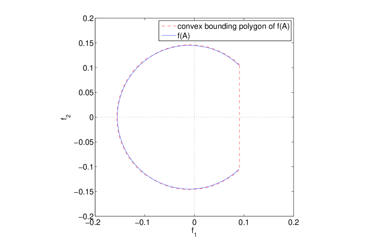
(b) The range $f(A)$ and its convex bounding polygon

Figure 1: The circular arc $A$ centered at $(u^{0},-\epsilon)$ that goes from $(u^{0}+r,v^{0}-r)$ to $(u^{0}-r,v^{0}-r)$ and its range $f(A)$ where $f$ is as in (22). Figure 1b shows that the bounding convex polygon of $f(A)$ contains the origin, and therefore $\bar{B}(x^{0},r)$ fails the convex bounding polygon test.

7 Time complexity analysis

In this section, we prove a number of theorems relating to the behavior of the KTS algorithm. We analyze the efficiency of KTS by showing that a patch either is a subset of a safe region, passes the Kantorovich test, or passes the exclusion test when it is smaller than a certain size that depends on the condition number of the function. Hence, we have the upper bound of the total number of patches examined by KTS in order to solve the intersection problem.

Recall that the Lipschitz constant $\hat{\omega}$ given by (14) is not the smallest Lipschitz constant of $f^{\prime}(x^{0})^{-1}f$ over $D^{\prime}$, where $D^{\prime}$ is given by (9). However, we can show that $\hat{\omega}\leq 4\theta\omega$, where $\omega$ denotes the smallest Lipschitz constant of $f^{\prime}(x^{0})^{-1}f$ over $D^{\prime}$. Since $\hat{\omega}$ is computed from the endpoints of the bounding intervals of $\max_{x\in[l,h]^{2}}|\hat{g}^{\prime}_{ijk}(x)|$, by (5),

$$\hat{\omega} \leq 4\theta\max_{i,j,k}\max_{x\in[l,h]^{2}}\left|\hat{g}^{\prime}_{ijk}(x)\right|$$ (23)

$$= 4\theta\max_{i,j,k}\max_{x\in X}\left|g^{\prime}_{ijk}(x)\right|$$

$$\leq 4\theta\max_{x\in X}\left\|g^{\prime}(x)\right\|=4\theta\omega.$$

With this bound on $\hat{\omega}$, we can now analyze the behavior of the Kantorovich test.

Theorem 7.1.

Let $x^{0}$ be a point in $[0,1]^{2}$ such that $f^{\prime}(x^{0})$ is invertible. Let $x^{*}$ be a zero of $f$ that is contained in $\bar{B}(x^{0},r)$, where $r$ is the radius of the patch under consideration. The patch $X=\bar{B}(x^{0},r)\subseteq[0,1]^{2}$ passes the Kantorovich test if

$$r\leq\frac{\gamma(\theta)-1}{\gamma(\theta)\omega_{D^{\prime}}}.$$ (24)

Proof.

The first step is to show that $\eta\hat{\omega}\leq 1/4$, where $\hat{\omega}$ is as in (14). Since $r\leq 1/2$, $\bar{B}(x^{0},2\gamma(\theta)r)\subseteq D^{\prime}$. Observe that for any $x,y\in D^{\prime}$,

$$\left\|f^{\prime}(x^{0})^{-1}(f^{\prime}(x)-f^{\prime}(y))\right\| = \|\left(f^{\prime}(x^{*})^{-1}+(f^{\prime}(x^{0})^{-1}-f^{\prime}(x^{*})^{-1})\right)$$ (25)

$$\left(f^{\prime}(x)-f^{\prime}(y)\right)\|$$

$$\leq \left\|f^{\prime}(x^{*})^{-1}\left(f^{\prime}(x)-f^{\prime}(y)\right)\right\|+\|f^{\prime}(x^{*})^{-1}$$

$$(f^{\prime}(x^{*})-f^{\prime}(x^{0}))f^{\prime}(x^{0})^{-1}(f^{\prime}(x)-f^{\prime}(y))\|$$

$$\leq \omega_{D^{\prime}}\left\|x-y\right\|+\left\|f^{\prime}(x^{*})^{-1}(f^{\prime}(x^{*})-f^{\prime}(x^{0}))\right\|\cdot$$

$$\left\|f^{\prime}(x^{0})^{-1}(f^{\prime}(x)-f^{\prime}(y))\right\|$$

$$\leq \omega_{D^{\prime}}\left\|x-y\right\|+$$

$$\omega_{D^{\prime}}\left\|x^{*}-x^{0}\right\|\cdot\left\|f^{\prime}(x^{0})^{-1}(f^{\prime}(x)-f^{\prime}(y))\right\|$$

$$\leq \omega_{D^{\prime}}\left\|x-y\right\|+$$

$$\omega_{D^{\prime}}r\cdot\left\|f^{\prime}(x^{0})^{-1}(f^{\prime}(x)-f^{\prime}(y))\right\|.$$

Since (24) implies

$$1-\omega_{D^{\prime}}r\geq 1/\gamma(\theta)>0,$$ (26)

the inequality (25) becomes

$$\left\|f^{\prime}(x^{0})^{-1}(f^{\prime}(x)-f^{\prime}(y))\right\|\leq\left(\frac{\omega_{D^{\prime}}}{1-\omega_{D^{\prime}}r}\right)\left\|x-y\right\|.$$

Hence

$$\omega\leq\frac{\omega_{D^{\prime}}}{1-\omega_{D^{\prime}}r},$$ (27)

where $\omega$ is the smallest Lipschitz constant of $f^{\prime}(x^{0})^{-1}f^{\prime}$ over $D^{\prime}$.

Recall that $f(x^{*})=0$ and $X\subseteq D^{\prime}$. Observe that

$$\eta \equiv \left\|f^{\prime}(x^{0})^{-1}f(x^{0})\right\|$$ (28)

$$= \left\|f^{\prime}(x^{0})^{-1}(f(x^{0})-f(x^{*}))\right\|$$

$$\leq \left(\max_{x\in X}\left\|f^{\prime}(x^{0})^{-1}f^{\prime}(x)\right\|\right)\cdot\left\|x^{0}-x^{*}\right\|$$

$$\leq \left(\max_{x\in X}\left\|f^{\prime}(x^{0})^{-1}(f^{\prime}(x)-f^{\prime}(x^{0}))+f^{\prime}(x^{0})^{-1}f^{\prime}(x^{0})\right\|\right)\cdot r$$

$$\leq \left(\max_{x\in X}\left\|f^{\prime}(x^{0})^{-1}(f^{\prime}(x)-f^{\prime}(x^{0}))\right\|+1\right)\cdot r$$

$$\leq (\omega r+1)r.$$

Using (23), (24), (26), (27), and (28) together give

$$\eta\hat{\omega}\leq\frac{1}{4}.$$

The last step is to to verify the other condition that $\bar{B}(x^{0},\rho_{-})\subseteq\bar{B}(x^{0},2\gamma(\theta)r)$. Noting that $\sqrt{1-2h}\geq 1-2h$ for $0\leq h\leq 1/2$, it is seen that

$$\rho_{-}(\eta,\hat{\omega}) = \frac{1-\sqrt{1-2\eta\hat{\omega}}}{\hat{\omega}}$$

$$\leq 2\eta$$

$$\leq 2(\omega r+1)r$$

$$\leq 2\gamma(\theta)r.\qed$$

Next results are concerned with the size of the patch satisfying the exclusion test.

Lemma 7.2.

Let $f:\mathbb{C}^{n}\rightarrow\mathbb{C}^{n}$ be a polynomial function with generic coefficients. Assume that all zeros of $f$ are invertible. Let $x^{0}$ be a point in $\mathbb{R}^{n}$. If

$$\left\|f^{\prime}(x^{*})^{-1}f(x^{0})\right\|\leq\frac{1}{2\omega_{f}}$$ (29)

for all complex zeros $x^{*}$ of $f$, then there exists $\hat{x}^{*}$, a zero of $f$, such that

$$\left\|x^{0}-\hat{x}^{*}\right\| \leq \frac{1-\sqrt{1-2\omega_{f}\left\|f^{\prime}(\hat{x}^{*})^{-1}f(x^{0})\right\|}}{\omega_{f}}$$

$$\equiv \sigma(\hat{x}^{*},x^{0}).$$

Proof.

By the assumption that $f$ has generic coefficients, the polynomial $f$ has a finite number of zeros. Let $x^{*}_{1}$, $x^{*}_{2}$, …, $x^{*}_{d}$ be all the complex zeros of $f$. Recall that a multiple zero has singular Jacobian. Hence, $f$ has no multiple zeros by assumption.

Define the polynomial $\bar{f}(x)=f(x)-f(x^{0})$. Note that $x^{0}$ is a zero of $\bar{f}$. We apply the Kantorovich’s theorem for complex functions (see [5]) to each $x^{*}_{i}$ with respect to $\bar{f}$. For each $x^{*}_{i}$, we use $D=\bar{B}(x^{*}_{i},\rho_{*}(x^{*}_{i}))$ and $\omega=\omega_{f}$. Since $\eta\equiv\left\|\bar{f}^{\prime}(x^{*}_{i})^{-1}\bar{f}(x^{*}_{i})\right\|=\left\|f^{\prime}(x^{*}_{i})^{-1}f(x^{0})\right\|$, the assumption (29) guarantees that the condition $\eta\omega\leq 1/2$ is satisfied. The condition $\bar{B}(x^{*}_{i},\rho_{-})\subseteq D$ is also satisfied by the definition of $D$. Therefore, the Kantorovich theorem states that there is a zero of $\bar{f}$, call it $\bar{x}^{*}_{i}$, such that

$$\left\|\bar{x}^{*}_{i}-x^{*}_{i}\right\|\leq\sigma(x^{*}_{i},x^{0}).$$ (31)

Recall that, for any $j$, $x^{*}_{j}$ is the unique zero of $f$ in $\bar{B}(x^{*}_{j},\rho_{*}(x^{*}_{j}))$. Therefore,

$$\left\|x^{*}_{i}-x^{*}_{j}\right\|>\max\{\rho_{*}(x^{*}_{i}),\rho_{*}(x^{*}_{j})\},i\neq j.$$ (32)

But (31) and (32) together imply that

$$\bar{x}^{*}_{i}\neq\bar{x}^{*}_{j},i\neq j.$$ (33)

Hence the mapping $x^{*}_{i}\rightarrow\bar{x}^{*}_{i}$ is injective. But since $f$ has generic coefficients and $f$ and $\bar{f}$ are of the same degrees, $f$ has at least as many zeros as $\bar{f}$ [3]. This implies that $x^{0}=\bar{x}^{*}_{i}$, for some $i$. The lemma follows. ∎

Theorem 7.3.

Let $f(x)=f(u,v)$ be a polynomial system in basis $\phi_{i}(u)\phi_{j}(v)$ in two dimensions with generic coefficients. Let $x^{0}=(u^{0},v^{0})$ be a point in $[0,1]^{2}$ such that $f^{\prime}(x^{0})$ is invertible and $f(x^{0})\neq 0$, $x^{*}$ be the closest zero in $\mathbb{R}^{2}$ of $f$ to $x^{0}$, and $\delta$ denote $\left\|x^{0}-x^{*}\right\|$. Let $r>0$ be such that $\bar{B}(x^{0},r)\subseteq[0,1]^{2}$. Assume $\delta>\frac{1}{\omega_{f}}$. Define $\hat{f}(\hat{u},\hat{v})$ such that

$$\hat{f}(\hat{u},\hat{v})=f(\frac{2r}{h-l}\hat{u}-\frac{2hr}{h-l}+u^{0}+r,\frac{2r}{h-l}\hat{v}-\frac{2hr}{h-l}+v^{0}+r).$$ (34)

In other word, $\hat{f}$ is a polynomial in basis $\phi_{i}(u)\phi_{j}(v)$ that reparametrizes with $[l,h]^{2}$ the surface defined by $f$ over the patch $\bar{B}(x^{0},r)$. The bounding polygon of $\{\hat{f}(u,v):l\leq u,v\leq h\}$ satisfying item 2 of the basis properties listed in Section 3 does not contain the origin if

$$r\leq\frac{1}{2\theta\mathop{\rm{cond}}(f)^{2}}.$$ (35)

Proof.

Let $X$ denote the patch $\bar{B}(x^{0},r)$ and $x$ denote an arbitrary point in $X$. Since $\delta>\frac{1}{\omega_{f}}$, the contrapositive of Lemma 7.2 implies there exists a zero $\bar{x}^{*}$ of $f$ satisfying $\left\|f^{\prime}(\bar{x}^{*})^{-1}f(x^{0})\right\|>\frac{1}{2\omega_{f}}$. Therefore, the condition (35) implies

$$r \leq \frac{1}{2\theta\mathop{\rm{cond}}(f)^{2}}$$

$$\leq \frac{1}{2\theta\omega_{f}\left\|f^{\prime}(\bar{x}^{*})^{-1}f^{\prime}(x)\right\|}$$

$$< \frac{\left\|f^{\prime}(\bar{x}^{*})^{-1}f(x^{0})\right\|}{\theta\left\|f^{\prime}(\bar{x}^{*})^{-1}f^{\prime}(x)\right\|}.$$

More specifically, we have

$$r<\frac{\left\|f^{\prime}(\bar{x}^{*})^{-1}f(x^{0})\right\|}{\theta\max_{y\in X}\left\|f^{\prime}(\bar{x}^{*})^{-1}f^{\prime}(y)\right\|},$$

which is equivalent to

$$\theta\cdot\max_{y\in X}\left\|f^{\prime}(\bar{x}^{*})^{-1}f^{\prime}(y)\right\|\cdot r<\left\|f^{\prime}(\bar{x}^{*})^{-1}f(x^{0})\right\|.$$ (36)

Recall that $\max_{y\in X}\left\|f^{\prime}(\bar{x}^{*})^{-1}f^{\prime}(y)\right\|$ is the Lipschitz constant for $f^{\prime}(\bar{x}^{*})^{-1}f$ on $X$. Hence, for any $x\in X$,

$$\left\|f^{\prime}(\bar{x}^{*})^{-1}f(x)-f^{\prime}(\bar{x}^{*})^{-1}f(x^{0})\right\| \leq \max_{y\in X}\left\|f^{\prime}(\bar{x}^{*})^{-1}f^{\prime}(y)\right\|\cdot\left\|x-x^{0}\right\|$$ (37)

$$\leq \max_{y\in X}\left\|f^{\prime}(\bar{x}^{*})^{-1}f^{\prime}(y)\right\|\cdot r.$$

Combining (36) and (37) gives

$$\theta\cdot\left\|f^{\prime}(\bar{x}^{*})^{-1}f(x)-f^{\prime}(\bar{x}^{*})^{-1}f(x^{0})\right\|<\left\|f^{\prime}(\bar{x}^{*})^{-1}f(x^{0})\right\|,$$

which is equivalent to

$$\theta\cdot\left\|f^{\prime}(\bar{x}^{*})^{-1}\hat{f}(\hat{x})-f^{\prime}(\bar{x}^{*})^{-1}\hat{f}(\hat{x}^{0})\right\|<\left\|f^{\prime}(\bar{x}^{*})^{-1}\hat{f}(\hat{x}^{0})\right\|$$

for some $\hat{x}\in[l,h]^{2}$, where $\hat{x}$ is the rescaled $x$ and $\hat{x}^{0}$ is the rescaled $x^{0}$ according to (34). In particular,

$$\theta\cdot\max_{\hat{x}\in[l,h]^{2}}\left\|f^{\prime}(\bar{x}^{*})^{-1}\hat{f}(\hat{x})-f^{\prime}(\bar{x}^{*})^{-1}\hat{f}(\hat{x}^{0})\right\|<\left\|f^{\prime}(\bar{x}^{*})^{-1}\hat{f}(\hat{x}^{0})\right\|.$$ (38)

Let $h(\hat{x})\equiv f^{\prime}(\bar{x}^{*})^{-1}\hat{f}(\hat{x})$ and $g(\hat{x})\equiv h(\hat{x})-h(\hat{x}^{0})$. By (5),

$$\left\|z\right\|\leq\theta\cdot\max_{\hat{x}\in[l,h]^{2}}\left\|g(\hat{x})\right\|,$$ (39)

for any $z$ in the bounding polygon $P_{g}$ of $\{g(\hat{x}):\hat{x}\in[l,h]^{2}\}$. Since the bounding polygon is required to be translationally invariant (item 2 of the basis properties listed in Section 3), (39) is equivalent to

$$\left\|y-h(\hat{x}^{0})\right\|\leq\theta\cdot\max_{\hat{x}\in[l,h]^{2}}\left\|h(\hat{x})-h(\hat{x}^{0}))\right\|,$$ (40)

for any $y$ in the bounding polygon $P_{h}$ of $\{h(\hat{x}):\hat{x}\in[l,h]^{2}\}$. Substituting (40) into the left hand side of (38) yields

$$\left\|y-h(\hat{x}^{0})\right\|<\left\|h(\hat{x}^{0})\right\|,$$ (41)

which implies that $P$ does not contain the origin. Since $f^{\prime}(\bar{x}^{*})^{-1}$ is invertible and the bounding polygon is affinely invariant, the bounding polygon of $\{\hat{f}(\hat{x}):\hat{x}\in[l,h]^{2}\}$ does not contain the origin, either. ∎

Theorem 7.4.

Let $f(x)=f(u,v)$ be a polynomial system in basis $\phi_{i}(u)\phi_{j}(v)$ in two dimensions with generic coefficients whose zeros are sought. Let $X=\bar{B}(x^{0},r)$ be a patch under consideration during the course of the KTS algorithm. The algorithm does not need to subdivide $X$ if

$$r\leq\frac{1}{2}\cdot\min\left\{\frac{1-1/\gamma(\theta)}{\omega_{f}},\frac{1}{2\theta\mathop{\rm{cond}}(f)^{2}}\right\}.$$ (42)

Proof.

If $\delta>1/\omega_{f}$, where $\delta$ is the distance between $x^{0}$ and the closest zero $x^{*}$, $r\leq\left(1-1/\gamma(\theta)\right)/(2\omega_{f})$ implies that $X$ does not contain a zero. Therefore, $r\leq 1/(4\theta\mathop{\rm{cond}}(f)^{2})$ implies that $X$ is excluded by the exclusion test according to Theorem 7.3.

Observe that $\omega_{*}\leq\omega_{f}$. If $\delta\leq\frac{1}{\omega_{f}}$, for any $x\in X$,

$$\left\|x-x^{*}\right\| \leq \left\|x-x^{0}\right\|+\left\|x^{0}-x^{*}\right\|$$

$$\leq r+\delta$$

$$\leq \frac{1-1/\gamma(\theta)}{\omega_{f}}+\frac{1}{\omega_{f}}$$

$$< \frac{2}{\omega_{f}}\leq\frac{2}{\omega_{*}}=\rho_{*}.$$

In other word, $X$ is contained within $\bar{B}(x^{*},\rho_{*})$, a safe region and therefore is excluded, provided that $x^{*}$ is found before $X$ is checked against all safe regions. By Theorem 7.1, $x^{*}$ is found by a region of size $2r\leq(1-1/\gamma(\theta))/\omega_{D^{\prime}}$. Since KTS examines larger regions before smaller ones, $x^{*}$ is found before $X$ is checked against safe regions. ∎

It should be noted that

$$1-1/\gamma(\theta)\geq 1/(18\theta)$$ (43)

hence both terms of the right hand side of (42) are asymptotically linear in $1/\theta$. The inequality (43) follows from the fact that

$$\sqrt{1+a}\leq 1+a/2-a^{2}/9$$ (44)

for any $a\in[0,1/4]$. To prove (44), simplify (44) to $a^{2}-9a+9/4\geq 0$, whose left hand side is a convex quadratic polynomial that crosses the x-axis at $(9-6\sqrt{2})/2\approx.2574$ and at $(9+6\sqrt{2})/2$.

8 Computational results

The KTS algorithm is implemented in Matlab and is tested against a number of problem instances with varying condition numbers. As Bézier surfaces are widely used in geometric modeling, we choose to implement KTS for the Bernstein basis case. Most of the test problems are created by using normally distributed random numbers as the coefficients $c_{ij}$’s of $f$. For some of the test problems especially those with high condition number, some coefficients are manually entered. The degrees of the test polynomials are between biquadratic and biquartic. As an example, the test case with $\mathop{\rm{cond}}(f)=3.5\times 10^{3}$ is $c_{00}=(1.2,.5)^{T}$, $c_{01}=(-.6,-.6)^{T}$, $c_{02}=(.1,1.1)^{T}$, $c_{10}=(-1.1,-.3)^{T}$, $c_{11}=(.6,-2.3)^{T}$, $c_{12}=(-2,-.1)^{T}$, $c_{20}=(.6,1.2)^{T}$, $c_{21}=(-1.1,-1.2)^{T}$, and $c_{22}=(-.5,.4)^{T}$. This is the test problem for the result in the second row of Table 2.

For the experiment, we use the algorithm by Jónsson and Vavasis [9] to compute the complex zeros required to estimate the condition number. Table 2 compares the efficiency of KTS with its condition number. The total number of subpatches examined by KTS during the entire computation, the width of the smallest patch among those examined, and the maximum number of Newton iterations (in the cases with more than one zero) to converge to a zero are reported. The result shows that KTS needs to examine more number of patches and needs to subdivide to smaller patches as the condition number becomes larger. Note that the high number of Newton iterations of some test cases is due to roundoff error.

	Num. of	Distance	Num. of	Smallest	Max. num. of
$\mathop{\rm{cond}}(f)$	zeros	between two	patches	width	Newton
		closest zeros	examined		iterations
$6.0\times 10^{2}$	1	-	21	.0625	3
$3.5\times 10^{3}$	2	.4196	29	.0625	3
$8.3\times 10^{4}$	2	.6638	33	.0625	3
$1.6\times 10^{5}$	1	-	41	.03125	4
$2.2\times 10^{7}$	3	.3624	57	.03125	4
$1.3\times 10^{8}$	4	.2806	81	.015625	6
$1.9\times 10^{9}$	4	.3069	69	.03125	6
$2.0\times 10^{10}$	2	.7810	105	.015625	6
$2.9\times 10^{11}$	1	-	257	.0039	9

Table 2: Efficiency of KTS algorithm on problems of different condition numbers.

9 Conclusion and future directions

We present KTS algorithm for finding the intersections between a parametric surface and a line. By using the combination of subdivision and Kantorovich’s theorem, our algorithm can take advantage of the quadratic convergence of Newton’s method without the problems of divergence and missing some intersections that commonly occur with Newton’s method. We also show that the efficiency of KTS has an upper bound that depends solely on the conditioning of the problem and the representation of the surface. Nevertheless, there are a number of questions left unanswered by this article such as

• Extensibility to piecewise polynomial surfaces and/or NURBS. Since KTS only requires the ability to compute the bounding polygon of a subpatch that satisfies the list of basis properties, it may be possible to extend KTS to handle these more general surfaces if bounding polygons having similar properties can be computed relatively quickly.

• Tighter condition number. The condition number presented earlier seems overly loose. It is likely that a tighter condition number exists. If a tighter condition number is found, we would be able to calculate a tighter bound on the time complexity of KTS, too.

• The necessity of the generic coefficients assumption. Is it possible to analyze the efficiency of KTS without this assumption?

• Using KTS in floating point arithmetic. In the presence of roundoff error, we may need to make adjustments for KTS to be able to guarantee that all zeros are found. In addition, the accuracy of the computed zeros would become an important issue in this case.

• Choice of polynomial basis. It is evident from Table 1 that the Chebyshev basis has the best (smallest) value of $\theta$, and therefore ought to require the fewest number of subdivisions. Our preliminary computational results [17] comparing bases, however, do not indicate a clear-cut advantage for the Chebyshev basis. Therefore, the impact of the choice of basis on practical efficiency is an interesting topic for further research.

References

- [1] W. Barth and W. Stürzlinger. Efficient ray-tracing for Bézier and B-spline surfaces. Computers and Graphics, 17(4):423–430, 1993.
- [2] Peter Deuflhard and Gerhard Heindl. Affine invariant convergence theorems for Newton’s method and extensions to related methods. SIAM J. Numer. Anal., 16:1–10, 1980.
- [3] I. Z. Emiris and J. F. Canny. Efficient incremental algorithms for the sparse resultant and the mixed volume. J. Symb. Comput., 20:117–149, 1995.
- [4] Gerald Farin. Curves and Surfaces for CAGD: A Practical Guide, fifth edition, Academic Press, 2002.
- [5] Rida T. Farouki, Bethany K. Kuspa, Carla Manni, and Alessandra Sestini. Efficient solution of the complex quadratic tridiagonal system for PH quintic splines. Numerical Algorithms, 27:35–60, 2001.
- [6] Alain Fournier and John Buchanan. Chebyshev polynomials for boxing and intersections of parametric curves and surfaces. Computer Graphics Forum, 13(3):C-127–C-142, 1994.
- [7] Robert M. Freund and Jorge R. Vera. Condition-Based Complexity of Convex Optimization in Conic Linear Form via the Ellipsoid Algorithm. SIAM J. Optim., 10:155–176, 1999.
- [8] Gene H. Golub and Charles F. Van Loan. Matrix Computations, third edition, the Johns Hopkins University Press, 1996.
- [9] G. Jónsson and S. Vavasis. Accurate solution of polynomial equations using Macaulay resultant matrices. Mathematics of Computation, 74:221 -262, 2005.
- [10] James T. Kajiya. Ray tracing parametric patches. Computer Graphics (SIGGRAPH ’82 Proceedings), 16(3):245–254, 1982.
- [11] L. Kantorovich. On Newton’s method for functional equations (Russian). Dokl. Akad. Nauk SSSR, 59:1237–1240, 1948.
- [12] Daniel Lischinski and Jakob Gonczarowski. Improved techniques for ray tracing parametric surfaces. The Visual Computer, 6:134–152, 1990.
- [13] T. Nishita, T. W. Sederberg, and M. Kakimoto. Ray tracing trimmed rational surface patches. ACM Computer Graphics, 24(4):337–345, 1990.
- [14] K. H. Qin, M. L. Gong, Y. J. Guan, and W. P. Wang. A new method for speeding up ray tracing NURBS surfaces. Computers and Graphics, 21(5):577–586, 1997.
- [15] Seven M. Rubin and Turner Whitted. A 3-dimensional representation for fast rendering of complex scenes. Computer Graphics (SIGGRAPH ’80 Proceedings), 14(3):110–116, 1980.
- [16] E. C. Sherbrooke and N. M. Patrikalakis. Computation of the solutions of nonlinear polynomial systems. Computer Aided Geometric Design, 10(5):379–405, 1993.
- [17] G. Srijuntongsiri and S. A. Vavasis. Properties of polynomial bases used in a line-surface intersection algorithm, http://arxiv.org/abs/0707.1515, 2007.
- [18] M. A. J. Sweeney and R. H. Bartels. Ray tracing free-form B-spline surface. IEEE Computer Graphics and Application, 6:41–49, 1986.
- [19] Kim-Chuan Toh and Lloyd N. Trefethen. Calculation of pseudospectra by the Arnoldi iteration. SIAM J. Sci. Comput., 17:1–15, 1996.
- [20] Daniel L. Toth. On ray tracing parametric surfaces. Computer Graphics (SIGGRAPH ’85 Proceedings), 19(3):171–179, 1985.
- [21] S. W. Wang, Z. C. Shih, and R. C. Chang. An efficient and stable ray tracing algorithm for parametric surfaces. Journals of Information Science and Engineering, 18(4):541–561, 2002.
- [22] Turner Whitted. An improved illumination model for shaded display. Communications of the ACM, 23(6):343–349, 1980.
- [23] C. G. Yang. On speeding up ray tracing of B-spline surfaces. Computer Aided Design, 19:122–130, 1987.