The Effect of Scheduling on Link Capacity in Multi-hop Wireless Networks

Abstract

Existing models of Multi-Hop Wireless Networks (MHWNs) assume that interference estimators of link quality such as observed busy time predict the capacity of the links. We show that these estimators do not capture the intricate interactions that occur at the scheduling level, which have a large impact on effective link capacity under contention based MAC protocols. We observe that scheduling problems arise only among those interfering sources whose concurrent transmissions cannot be prevented by the MAC protocol’s collision management mechanisms; other interfering sources can arbitrate the medium and co-exist successfully. Based on this observation, we propose a methodology for rating links and show that it achieves high correlation with observed behavior in simulation. We then use this rating as part of a branch-and-bound framework based on a linear programming formulation for traffic engineering in static MHWNs and show that it achieves considerable improvement in performance relative to interference based models.

I Introduction

Multi-hop wireless networks (MHWNs) play an increasingly important role at the edge of the Internet. Mesh networks provide an extremely cost-effective last mile technology for broadband access, ad hoc networks have many applications in the military, industry and everyday life, and sensor networks hold the promise of revolutionizing sensing across a broad range of applications and scientific disciplines – they are forecast to become bridges between the physical and digital worlds. This range of applications results in MHWNs with widely different properties in terms of scales, traffic patterns, radio capabilities and node capabilities. Thus, effective networking of MHWNs has attracted significant research interest.

Gupta and Kumar [1] derived the asymptotic capacity of MHWNs under the assumptions of idealized propagation, uniformly distributed sources and destinations, and an optimal routing and packet transmission schedule. A key observation in deriving this limit is that the available bandwidth between a pair of communicating nodes is influenced not only by the nominal communication bandwidth, but also by ongoing communication in nearby regions of the network due to interference.

While the asymptotic limit is useful, the analysis cannot be applied to evaluate, or traffic engineer specific networks and traffic patterns. Recently, several efforts to model MHWNs while incorporating the effect of interference have been carried out  [2, 3, 4]. One of the important limitations in these works is that they abstract away scheduling, for example, by ignoring its effect or assuming the presence of an omniscient scheduler. Existing works in this area use an estimate of interference to assess the quality of links for use in estimating capacity or determining effective globally coordinated routing configurations. We present these and other related works in Section II.

The first contribution of the paper is to show (in Section III) that commonly used metrics for capacity provide only an upper bound on the achievable capacity of a link. Scheduling effects, which are not accounted for by these metrics, play an important, often defining, role in determining the effective capacity of a link. The effects arise from the inability of practical contention based MAC protocols, such as IEEE 802.11, to prevent collisions in some cases. We show that metrics such as observed percentage of MAC level timeouts, can estimate the scheduling effect on capacity, and when combined with the interference metrics provide accurate estimates of link quality.

It is not readily clear how to estimate the expected scheduling interactions among a given set of active links. The second contribution of the paper is an analysis of this problem and a proposed model for estimating the scheduling effects. We build on the observation that virtually all collisions are caused only by the subset of interfering sources whose concurrent transmission cannot be prevented by the MAC protocol, due to the imprecise nature of collision prevention mechanisms in contention based MAC; other interfering sources are able to handshake effectively and avoid collisions. We develop a model for identifying these sets of nodes and predicting the quality of a given link. We show that proposed metrics effectively predict the expected percentage of MAC timeouts. The analysis and the development of scheduling aware metrics are presented in Section IV.

To demonstrate the effectiveness of the proposed metrics, we extend a linear programming formulation for global route planning in MHWNs to use the scheduling-aware metrics. We show that the resulting routes achieve large performance improvements relative to routes obtained considering interference metrics only; the improvement is even larger with respect to a greedy routing protocol such as DSR. The algorithm is presented in Section V and the experimental evaluation is presented in Section IV-D.

The centralized approach of the model is useful for analysis and for static networks (e.g., mesh networks), but not directly for dynamic networks. However, we believe that identifying the nature and scope of interactions provides an excellent starting point for developing distributed algorithms that result in effective routing configurations in dynamic networks. We present our conclusions and future research directions in Section VI.

II Related work

A primary challenge of efficient channel usage for the emerging applications in MHWNs would be to identify the critical metrics of routing protocol that enables to approximate an optimal route configuration.Under idealized assumptions, hop count has been experimentally shown to determine a stand-alone connection performance metric  [5]. The validity of hop-count as a sole metric of path quality is brought into question because it fails to account for two crucial factors: the channel state between the sender and receiver (assumed perfect within transmission range) and interference from other connections (which is ignored when taking routing decisions). It does not capture the underlying MAC and physical layer which has a great effect on the routing protocol [6, 7]. Using the shortest number of hops often lead to the choice of distant next-hop, thus reducing signal strength and channel quality between the hops [8]. Researchers have studied approaches for estimating the quality of links including Round Trip Time (RTT) [9] and the expected number of retransmissions (ETX) [10]. Draves et al. carried out a comparison of these and other metrics [11] and concluded that ETX is the most effective measure in their experimental static network. We believe that the scheduling interactions analyzed in the paper would reason the superior performance of ETX.

Various approaches and metrics has resulted in studies that not only identifies the parameters and their relationships but also quantifies them. Most of the studies use the notion of conflict graphs and maximal independent sets for capturing the wireless effects. Jain et al. and Kodialam et al.  [2, 3] propose an interference model and show the effect of interference on the aggregate throughput. However, they assume all-or-none interference and an optimal scheduler. While such interference aware routes spatially characterize the routes, the scheduling interactions studied in this paper capture the temporal properties of the routes. due to contention based scheduling.

Link behavior and routing protocols that account for realistic wireless channel state has been empirically studied in [12, 13, 14, 15]. Garetto et al [16] estimate the effect of scheduling on the throughput of CSMA channels. They use a similar approach to ours in computing maximal cliques to identify concurrently transmitting nodes. However, unlike our approach, they use a Markovian model to estimate the scheduling effects statistically and use the simplified protocol model. In contrast, our model is more constructive in nature starting from the underlying causes of collisions.

III Link Capacity Metrics

In this section, we first show using a simple experiment that aggregate interference metrics provide only a coarse estimate of link quality, especially under medium to high interference, because they ignore the effect of scheduling. We simulate different sets of 144 uniformly distributed nodes with 25 arbitrarily chosen one-hop connections. The aim of this experiment is to show how the performance achieved by these connections correlates with existing capacity metrics. We chose one hop connections to eliminate multi-hop artifacts such as self-interference and pipelining and isolate link-level interactions. Each source sends CBR data at a rate high enough to ensure that it always has packets to send.

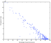
(a)

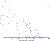
(b)

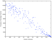
(c)

Figure 1: Effect of Interference and Scheduling on Capacity. (a) shows effect of source busy time on throughput; (b) enlarges the high interference region of (a); (c) shows that normalized throughput is a function of scheduling/MAC level timeouts.

The amount of time a source observes a busy channel is a commonly used estimate of the capacity available to the link. For example, if the MAC uses carrier sense, the sender will not send if the medium is busy. Intuitively, under an ideal scheduler, the throughput of the link will only be a function of the available transmission time (ATT). However, in practical CSMA/CA based schedulers, packet collisions and timeouts arise because perfect scheduling based on local information only is not possible. For example, the channel may be sensed idle, at the source, but a collision occurs at the destination. Thus, the observed throughput will be a function of the available capacity as well as the scheduling interactions.

Figure 1(a) plots the busy time against the observed throughput of the link. In general, as interference increases, the achievable capacity decreases. However, it can be seen that at higher busy times (enlarged for clarity in Figure 1(b)), large variations in throughput arise for the same observed busy time.

With increasing interference, the scheduling effectiveness starts to play a determining effect on the throughput of the link. Let $t_{i}$ be the throughput achieved by an ideal scheduler; intuitively $t_{i}$ is proportional to the amount of available transmission time (ATT). Let $t_{o}$ be the observed throughput in the CSMA based scheduler, IEEE 802.11. The ratio of $\frac{t_{o}}{t_{i}}$, called normalized throughput provides a measure of the scheduling efficiency relative to an ideal scheduler independently of the available transmission time. Figure 1(c) plots the normalized throughput as a function of observed percentage of MAC level transmissions that experience RTS or ACK timeouts for all the links. It can be seen that as the fraction of packet timeouts increases, the normalized throughput decreases almost linearly. Thus the reason for variations in observed capacity from the nominal capacity predicted by the interference metric is the scheduling as observed in MAC level timeouts.

Aggregate interference metrics such as busy time cannot predict scheduling effects and correlate poorly with scheduling efficiency. As a result, in the next section, we analyze the problem of estimating the scheduling effects that a set of active links present to each other to develop link quality metrics capable of capturing both the interference and scheduling effects.

IV Modeling Scheduling Interactions

In this section, we develop models for estimating the effect of scheduling on the capacity of a link. A key observation that provides the starting point for this analysis is that the vast majority of collisions occur due to interfering links whose sources are not prevented from concurrent transmission by the MAC protocol; other interfering links that can handshake effectively through the MAC protocol are not impacted negatively by the scheduling effects.

In contention based protocols, the channel state at the receiver is not known at the sender which gives rise to the well-known hidden and exposed terminal problems [17]. To counter these effects, IEEE 802.11 uses an aggressive CSMA to attempt to prevent far-away interfering sources from transmitting together (but potentially preventing non-interfering sources from transmitting; hidden terminal is reduced, but exposed terminal increased). Despite this aggressive carrier sense value, not all potential hidden terminals are prevented. Optionally, the standard allows the use Collision Avoidance (CA), which consists of Request-to-Send (RTS)/Clear-to-Send (CTS) control packets, to attempt to reserve the medium. Thus, contention is carried out with small packets. However, CA only prevents interfering nodes in reception range of each other (a small subset of possible interferers) and is often not enabled in real deployments. Thus, neither CSMA nor CA block prevent all potential collisions, which gives rise to the destructive scheduling interactions being studied in this paper. We note that many radios turn off the CA mechanism, increasing collision potential and the effect of scheduling. In this paper, we model the case with CA enabled; modeling the case with CA disabled is simpler and similar to the ACK timeout portion of the model.

IV-A Preliminaries

Let $G(V,E)$ be a graph representing the network where $V$ is the set of all the nodes and $E$ is the set of active links. Let $\Theta_{ij}$ be a $n$x$n$ matrix, representing the signal strength observed at node $j$ for node $i$’s transmission. Under ideal power-law signal propagation assumptions, $\Theta_{ij}$ can be derived based on node location. However, it may be defined according to other propagation models or experimentally derived based on observed connectivity and interference.

We show the derivation assuming that the RTS/CTS handshake is enabled (which is the more difficult case). However, it is possible to investigate performance without this handshake since disabling the handshake is becoming more common in practice [18]. We showed in Section III that collisions accurately predict the effect of scheduling on capacity; they are the primary indicators of inefficient scheduling. In addition to wasted channel time, they result in back-offs, which may cause the channel to become idle.

At the source, collisions are observed in one of two ways: an RTS Timeout (indicating a loss of RTS or absence/loss of CTS) or a DATA timeout (indicating a loss of DATA or ACK). The root cause of collisions is the presence of sources that can transmit concurrently but that interfere with each other’s destinations; ideally the MAC protocol would have prevented all but the non-interfering sources from transmission. We break the problem into two parts: (1) identifying the links whose senders can transmit concurrently despite the protocol’s handshake; and (2) Quantifying how these links interact.

IV-B Identifying Concurrently Transmitting Senders

We define the notion of a Maximal Independent Contention Set (MICS) as a set of links whose sources are not prevented from initiating transmissions while there are active transmissions on the other links of the same MICS. Due to the imperfect nature of MAC handshake, links that interfere may belong in the same MICS. Thus, collisions occur due to interactions within an MICS (except for rare race conditions), transmissions across different MICS’ are prevented by the MAC protocol. The definition of an MICS follows.

• A set $C\subseteq E$ forms a Maximal Independent Contention Set (MICS) if $\forall(s,d)\in C,\nexists(s_{2},d_{2})\in E-C\text{ such that }\\ \Theta_{s_{2}d}+\displaystyle\sum_{(s_{1},d_{1})\in C,(s_{1},d_{1})\neq(s,d)}\Theta_{s_{1}d}<{\rm T}_{RX}-W$.
  A set of all MICS is denoted by $\rm M$.

A set of all the MICS in which a given link $(s,d)$ is present is denoted by $N_{(s,d)}$ (Equation 1).

$${N}_{(s,d)}=\{C|C\in\rm M,(s,d)\in C\}$$ (1)

The probability that MICS $C$ is currently active is represented as ${\mu}_{C}$. Precise formulation of ${\mu}_{C}$ requires estimation of different factors like: (1) the dependence of MICS on the initiation order of sources; and (2) the sequence of interactions between the conflicting sources (probably cyclic). An approximation of ${\mu}_{C}$ is desirable since an accurate estimation of all the factors makes the model computationally infeasible. We use the approximation in Equation 2 which assumes that the set of sources capable of initiating concurrent transmissions compete independently from each other. The probability of a MICS occurring is dependent upon the number of sources present in the MICS. Thus, the approximation makes all MICS’ of the same size equi-probable, with the probability of a MICS increasing with the number of edges in it.

$$\mu_{C}=\frac{|C|}{\sum_{C^{\prime}\in\rm M}|C^{\prime}|}$$ (2)

Improving the characterization of MICS activation probabilities is an area of further refinement of the model.

IV-C Quantifying Link Interactions

The majority of the timeouts occur due the interaction among the sources which do not prevent each other from transmission via CSMA or CA. MICS characterize such groups of sources. Evaluating link interactions is therefore simplified into evaluating interactions on a per-MICS basis and then weighting these by the probability of MICS activation in Equation 2. The overall timeouts experienced by a link is a function of the the packet timeouts due to interaction in all the MICS in which the link is present. In this section, we model the problem at two levels: (1) Interactions between the links of the MICS; and (2) A weighting function across MICS to measure the overall timeouts. While we use the IEEE 802.11, the analysis can be adapted to other contention based protocols.

Estimating RTS Timeouts

An RTS timeout occurs for one of three reasons: (1) an RTS collision; (2) a busy receiver not responding to the RTS due to physical or virtual carrier sensing being active at the destination; or (3) a CTS collision.

Consider an RTS timeout at a link $(s,d)$. Since the noise at $s$ is below ${\rm T}_{RX}$ before the RTS initiation (otherwise, the link is not part of the currently active MICS) and $d$ should respond with CTS immediately upon reception of RTS, the chances of CTS collision are low. This intuition was validated by extended observation of MAC traces in simulation. Hence, an RTS collision or a busy channel at the receiver are the candidates for causing an RTS timeout.

In a given MICS $C$, an Unsafe Link $(s_{1},d_{1})$ for a link $(s,d)$ is given by Equation IV-C and is defined as a link whose transmission at source ($s_{1}$) may create a busy channel at the receiver $d$ (condition 1 of Equation IV-C) or cause an RTS collision (condition 2). Both the cases results in an RTS Timeout.

$${\rm U}^{C}_{(s,d)}=\Bigl{\{}(s_{1},d_{1})\mid(s_{1},d_{1})\in C,$$

$$\Theta_{s_{1}d}\geq{\rm T}_{RX}-W\text{ or }\frac{\Theta_{sd}}{\Theta_{s_{1}d}+W}<{\rm T}_{SINR}\Bigr{\}}$$ (3)

A limitation of the current formulation is that we do not consider the effect of timeouts due to the virtual carrier sense being set at the receiver. While a substantial number of RTS timeouts were due to the VCS (around 25% as explained later in IV-D1), modeling this effect requires estimating: (1) Packet capture ability of the node under a given MICS (which cannot be assumed to be a constant “reception threshold” as done in Protocol Model of interference); (2) Distinguishing the timeouts due to “False VCS” which may turn on the VCS even if the competing packet transfer is unsuccessful (that is, an RTS may cause a sender to defer, even if its CTS was never received – we call this “false VCS” effect). A deeper study of VCS related effects is an area of extension of the model.

The number of RTS Timeouts for a link $(s,d)$ depends upon the number of unsafe links that can be initiated before the link $(s,d)$. Deriving the probabilities of such initiations is done as follows: Let $p_{e}(k)$ be the probability that exactly $k$ links will initiate transmission before a given link. It can be shown that this probability is given by $p_{e}(k)=\frac{1}{k+1}$. Let $p(k)$ be the probability that at least one of the $k$ links will initiate transmission before any given link. It can be shown that $p(k)=\sum_{i=1}^{k}{(-1)}^{(i-1)}{k\choose i}p_{e}(k)$. Given $k$ unsafe links, $p(k)$ indicates the probability that at least one of the unsafe link has initiated before the link $(s,d)$. A cumulative metric to measure the percentage of the RTS Timeouts should be unbiased to the number of MICS to which the link belongs. We approximate the such a metric by ${{\cal{R}}}_{s,d}$.

• We define the following Interaction Based RTS Link Rating (${\cal{R}}_{(s,d)}$) for a link $(s,d)$:
  ${{\cal{R}}}_{(s,d)}=\dfrac{\displaystyle\sum_{C\in\rm M}p(|{\rm U}^{C}_{(s,d)}|)}{|{N}_{(s,d)}|}$

Estimating ACK Timeouts

More important than RTS timeouts are collisions affecting DATA or ACK packets which result in ACK timeouts. ACK timeouts are costly since they denote unsuccessful communication after a prolonged period of channel usage. Considering that the ACK will be sent immediately after DATA transmission, the probability of the ACK collision at the source is small. Hence we formulate the ACK timeouts due to DATA packet corruption. The basis for modeling ACK timeouts is to determine the links that can corrupt an ongoing DATA packet by RTS, CTS or ACK packet. We define a set of links that can corrupt the DATA transmission of the link $(s,d)$ by initiating an RTS by ${\rm K}_{(s,d)}$ as given in Equation IV-C. These are the set of links $(s_{1},d_{1})$ which co-exist in any of the MICS of the link and the RTS from $s_{1}$ could corrupt the data packet at $d$.

$${\rm K}_{(s,d)}=\Bigl{\{}(s_{1},d_{1})\mid\exists C\in\rm M\text{ such that }$$

$$(s,d),(s_{1},d_{1})\in C,\frac{\Theta_{sd}}{\Theta_{s_{1},d}+W}<{\rm T}_{SINR}\Bigl{\}}$$ (4)

Similar to ${\rm K}$, the sets of links that can corrupt the DATA packet by transmitting CTS or ACK are represented as $\bar{\rm K}_{(s,d)}$ and $\ddot{\rm K}_{(s,d)}$ respectively. To determine the set $\bar{\rm K}_{(s,d)}$, we place the restriction that RTS does not corrupt the data packet to ensure that the same DATA packet drop is not accounted twice, in ${\rm K}_{(s,d)}$ and $\bar{\rm K}_{(s,d)}$. Equation 5 shows the set of links that can corrupt the packet of the link $(s,d)$ by CTS transmission.

$$\bar{\rm K}_{(s,d)}=\{(s_{1},d_{1})\mid\exists C\in\rm M\text{ such that }$$

$$(s,d),(s_{1},d_{1})\in C,(s_{1},d_{1})\not\in{\rm K}_{(s,d)},$$

$$\Theta_{sd_{1}}<{\rm T}_{RX}-N,\frac{\Theta_{sd}}{\Theta_{d_{1}d}+W}<{\rm T}_{SINR}\}$$ (5)

Similarly, the set of links that can corrupt the DATA packet by ACK transmission are defined in equation 6. There may be links whose CTS does not corrupt the DATA packet of but the ACK packet could corrupt since ACK transmission $\cal{T}$ A $\ddot{\rm K}_{(s,d)}$ for a given link is a set of links $(s_{1},d_{1})$ such that the links co-exist in the same MICS and $(s_{1},d_{1})$ does not belong to either ${\rm K}_{(s,d)}$ or $\bar{\rm K}_{(s,d)}$ and an RTS from either $(s,d)$ or $(s_{1},d_{1})$ does not corrupt the DATA packet of the other link, while the ACK packet from $d_{1}$ corrupts the DATA of $(s,d)$. There may be links $(s_{2},d_{2})$ whose CTS does not corrupt the DATA packet of $(s,d)$ because CTS initiation is canceled because of the channel being busy at $d_{2}$. However, if the scheduling of two links is such that $(s_{2},d_{2})$ starts before $(s,d)$ and $(s_{2},d_{2})$ ends before $(s,d)$ then the ACK packet of $d_{2}$ may corrupt the DATA packet at $d$ since ACK transmission happens without CCA.

$$\ddot{\rm K}_{(s,d)}=\{(s_{1},d_{1})\mid\exists C\in\rm M\text{ such that }(s,d),(s_{1},d_{1})\in C,$$

$$(s_{1},d_{1})\not\in{\rm K}_{(s,d)},(s_{1},d_{1})\not\in\bar{\rm K}_{(s,d)},$$

$$\frac{\Theta_{s_{1}d_{1}}}{\Theta_{sd_{1}}+W}>={\rm T}_{SINR},\frac{\Theta_{sd}}{\Theta_{d_{1}d}+W}<{\rm T}_{SINR}\}$$ (6)

While calculating the DATA drops, it is important to account for the cumulative interference produced by multiple concurrent links. This is because of the higher possibility of such combination of interference during the longer period of data transmission. Let $\nu_{C}^{(s,d)}$ be the probability that the interference from the links of the MICS $C$ corrupts the DATA packet. Calculation of $\nu_{C}^{(s,d)}$ requires the estimation of the interference caused to a node by multiple active links. In the next paragraph, we explain the estimation of the $\nu_{C}^{(s,d)}$ by capturing the cumulative interference.

Indirect Interference Edges $\rm I_{C}^{(s,d)}$ for a given edge $(s,d)$ in a given MICS $C$ is a set of links in $C$ whose transmission does not make the channel busy at $d$ (Equation IV-C). The maximum cumulative noise from indirect edges is the sum of maximum noises observed at $d$ by either $s_{1}$ or $d_{1}$(Equation 8). Simultaneous DATA transmissions by Indirect Interference Edges may create a busy channel.

$$\rm I_{C}^{(s,d)}=\Bigl{\{}(s_{1},d_{1})\mid(s_{1},d_{1})\in C,(s_{1},d_{1})\neq(s,d),$$

$$\Theta_{s_{1}d}+W<{\rm T}_{RX},\Theta_{d_{1}d}+W<{\rm T}_{RX}\Bigl{\}}$$ (7)

$$\eta_{C}^{(s,d)}=\sum_{\forall(s_{1},d_{1})\in\rm I_{C}^{(s,d)}}\operatorname{max}(\Theta_{s_{1}d},\Theta_{d_{1}d})$$ (8)

The cumulative interference factor (Equation 9) defines the effect on data transmission because of such combination of interference. If the interference $\eta^{C}_{(s,d)}$ does not corrupt the data packet, then the value $\nu^{C}_{(s,d)}$ is set to $0$. If it affects it then it is set to a value based on probability of MICS $C$ and the number of indirect interfering links (Equation 9).

$$\nu_{C}^{(s,d)}=\begin{cases}\mu_{C}p_{e}(|\rm I_{C}^{(s,d)}|)&\text{if }\frac{\Theta_{sd}}{(\eta_{C}^{(s,d)}+W)}<{\rm T}_{SINR}\\ 0,&\textit{otherwise.}\end{cases}$$ (9)

Finally, an estimate for the amount of ACK Timeouts is obtained by accounting for the links that corrupt DATA packet by RTS, CTS, ACK in addition to indirectly interfering links as given in Equation 10. Since, the percentage of timeouts is of interest, the probability that the interfering links will corrupt the data packet also depends upon ratio of the probability of the source winning in a given MICS. The probability of the source of the link $(s,d)$ winning the channel is denoted by $\sigma_{(s,d)}$ and is given by the sum of all the probability of the MICS winning the channel in which the link is present.

$${\cal{D}}_{(s,d)}=\dfrac{\displaystyle\sum_{\forall C\in\rm M}\mu_{C}.p(|{\rm K}_{C}|+|\bar{\rm K}_{C}|+|\ddot{\rm K}_{C}|)+\nu_{C}^{(s,d)}}{\sigma_{(s,d)}}$$ (10)

Impact of Virtual Carrier Sense on ACK Timeouts

The formulation presented thusfar does not account for the effect of Virtual Carrier Sensing (VCS). More specifically, when an RTS or CTS is received by other nodes, these nodes defer from transmission even if the RTS or CTS ends up failing, meaning that the data transmission will not occur. Estimating VCS effect requires determination if a node can capture the RTS/CTS packets based on the signal to interference at the node. Under the SINR propagation model, the packet can be captured if the cumulative interference due to all the concurrent active links yields a SINR ratio greater than the ${\rm T}_{SINR}$.

In modeling this effect, and as a first order approximation, we ignore the possibility of simultaneous RTS or CTS packets (as observed in Section IV-D1) and consider only the DATA packets whose transmission causes extended interference time. The cumulative interference in a MICS cannot be calculated by summing up the interference experienced from all the sources of the MICS, since MICS includes the links which may suffer RTS Timeouts, thus not initiating the DATA transfer. Measuring cumulative interference due to concurrent DATA packet transmission can be done by computing the maximum independent set of links that can initiate the DATA transfer concurrently. We call such a set of links as Existent MICS (EMICS).

• A set $C^{\prime}\subseteq E$ is an Existent Maximal Independent Contention Set(EMICS) if:

  1. $\exists C\in\rm M\text{ such that }C^{\prime}\subseteq C\\$

  2. $\forall(s,d)\in C^{\prime}\text{ and }\forall(s_{1},d_{1})\in C^{\prime}\\ \displaystyle\sum_{(s_{1},d_{1})\neq(s,d)}\operatorname{max}(\Theta_{s_{1}d},\Theta_{d_{1}d})+W<{\rm T}_{RX}\\$

  3. $\forall(s,d)\in C^{\prime}\text{ and }\forall(s_{1},d_{1})\in C^{\prime}\\ \frac{\Theta_{sd}}{\displaystyle\sum_{(s_{1},d_{1})\neq(s,d)}\operatorname{max}(\Theta_{s_{1}d},\Theta_{d_{1}d})+W}\geq{\rm T}_{SINR}\\$

  4. $\forall(s,d)\in C^{\prime}\text{ and }\forall(s_{1},d_{1})\in C^{\prime}\\ \frac{\Theta_{ds}}{\displaystyle\sum_{(s_{1},d_{1})\neq(s,d)}\operatorname{max}(\Theta_{s_{1}s},\Theta_{d_{1}s})+W}\geq{\rm T}_{SINR}\\$

  A set of all EMICS is denoted by $\widehat{\rm M}$.

A link $(s,d)$ can be present in more than one EMICS, thus, the interference experienced at the node $a$ when the link $(s,d)$ is active will vary depending upon which EMICS is active. The maximum interference at the node $a$ when $(s,d)$ is active is the maximum of the sum of interference caused by links in EMICS of $(s_{1},d_{1})$. (Equation 11).

$$\rm P_{a,(s,d)}=\displaystyle\max_{\forall C^{\prime}\in\widehat{\rm M},(s,d)\in C^{\prime}}\Biggl{(}\displaystyle\sum_{(s_{1},d_{1})\in C^{\prime}}\Theta_{as_{1}}\Biggr{)}$$ (11)

We approximate that the node $a$ can set its VCS to the RTS or CTS of link $(s,d)$ if the noise at $a$ is lesser than $\rm P_{a,(s,d)}$. This is given by $\beta_{a,(s,d)}$ in Equation 12.

$$\beta_{a,(s,d)}=\begin{cases}1&\text{if }\operatorname{max}(\Theta_{as},\Theta_{ad})>{\rm T}_{RX}\text{ and }\\ ~{}&~{}~{}~{}\frac{\operatorname{max}(\Theta_{as},\Theta_{ad})}{\rm P_{a,(s,d)}}\geq{\rm T}_{SINR}\\ 0,&\textit{otherwise.}\end{cases}$$ (12)

We redefine the set of links that can corrupt the data packet by transmitting RTS or CTS based on the VCS and denote the sets by ${\widehat{{\rm K}}}_{C}$ and ${\widehat{\bar{\rm K}}}_{C}$ as given in Equations 13 and 14.

$${\widehat{{\rm K}}}_{(s,d)}=\{(s_{1},d_{1})\mid(s_{1},d_{1})\in{\rm K}_{(s,d)},\beta_{s_{1},(s,d)}=0\}$$ (13)

$${\widehat{\bar{\rm K}}}_{(s,d)}=\{(s_{1},d_{1})\mid(s_{1},d_{1})\in\bar{\rm K}_{(s,d)},\beta_{d_{1},(s,d)}=0\}$$ (14)

The ACK Timeout Rating accounting for the VCS is given in Equation 15.

$$\widehat{{\cal{D}}}_{(s,d)}=\dfrac{\displaystyle\sum_{\forall C\in\rm M}\mu_{C}.p(|{\widehat{{\rm K}}}_{C}|+|{\widehat{\bar{\rm K}}}_{C}|+|\ddot{\rm K}_{C}|)+\nu_{C}^{(s,d)}}{\sigma_{(s,d)}}$$ (15)

All the demonstrated results use VCS enabled ACK Timeout rating.

Complexity Analysis

Contention among the links can be mapped into a Contention Graph $G(V^{\prime},E^{\prime})$ where the vertices represent the active links and the edges denote the contention. An edge is present between two vertices $a,b\in V^{\prime}$ if the source’s of $a$ and $b$ can initiate concurrent transmission [2] under contention based scheduling. The computation of the set of MICS($\rm M$) is the problem of finding all the Maximal Independent Sets (MIS’) in $G^{\prime}$ (all the Maximal Cliques in the complementary graph $\bar{G^{\prime}}$). The problem of finding MIS is NP-complete. The number of MIS in a graph is denoted by $l_{\rm M}$, which is bounded by $O(3^{\frac{n}{3}})$[19]. We used an iterative heuristic [2] for finding independent sets. The algorithm implemented has a complexity of $O(l_{\rm M}n^{3})$ where $n=|V^{\prime}|$, the number of active links. The approximate algorithm without considering the effect of VCS (Section IV-C) has $O(l_{\rm M}n^{2}\log(n))$ complexity.

IV-D Experimental Validation

This section validates MICS interactions, which form the basis of the formulation, with the interactions observed in the simulation. We evaluate the ability of the IBLR metrics to predict MAC collisions in Section IV-D2.

IV-D1 Validation of MICS Interaction

The link quality formulation results were analyzed and were compared with the simulation results. We altered the QualNet simulator [20] to account for the SINR Threshold model. Ten different scenarios, each with a random placement of 144 nodes in a 1600m$\times$1600m area was chosen with 25 one-hop connections (250 active links).

Figure 2(a) compares the simulation results of the causes for packet timeouts (X-axis) to the average number of instances on Y-axis. RTS-A and RTS-I stands for the RTS packet collision during the arrival and intermediate stage of the RTS packet. Similarly, DATA-A and DATA-I stands for the DATA packet collision on arrival and at intermediate stage. The CTS-PCS and CTS-VCS denotes the CTS packet not being sent by the destination as a result of physical and virtual carrier sensing , respectively. Intra-MICS interactions are those due to two transmissions of the same MICS (which are captured by the formulation). Inter-MICS denotes transmissions that are not captured by the formulation and can be due to random effects of channel access like instantaneous transmissions. As we indicated earlier, Inter-MICS collisions are quite rare (2.67% in our results) with most occurring in the RTS-A and RTS-I stage. This validates the MICS framework for capturing the scheduling interactions. The intermediate DATA packet collisions indicate the ineffectiveness of the RTS-CTS handshake (including the VCS).

IV-D2 Effectiveness of the IBLR metrics

     

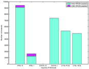
(a) Collision Causes

(b) RTS Timeouts

(c) ACK Timeouts

Figure 2: Validation and effectiveness of IBLR metrics

	${\cal{R}}$	$\cal{I}$	$\cal{T}$	$\cal{S}$
$R$	0.819	-0.121	0.655	-0.059
$\rho$	0.872	0.183	0.529	-0.404

TABLE I: Correlation of RTS Timeouts

	$\widehat{{\cal{D}}}$	$\cal{I}$	$\cal{T}$	$\cal{S}$
$R$	0.916	-0.071	0.262	-0.061
$\rho$	0.899	0.110	0.320	-0.558

TABLE II: Correlation of ACK Timeouts

In Figure 2(b) and 2(c), the IBLR RTS Timeout Rating(${\cal{R}}$) and ACK Timeout Rating ($\widehat{{\cal{D}}}$) of the formulation is plotted against the fraction of RTS Timeouts (ratio of RTS Timeouts to the total RTS transmissions) and ACK timeouts respectively. Table II compares the Correlation co-efficient ($R$) and Spearman’s Rank Coefficient ($\rho$) measured between the percentage of RTS Timeouts observed in the simulator to four commonly used metrics: (1) RTS Timeout Rating (${\cal{R}}$), (2) Interference Level ($\cal{I}$) measurement at receiver , (3) the Busy Time($\cal{T}$) at the receiver, and (4) Signal-to-Interference Noise Ratio ($\cal{S}$). Interference Level($\cal{I}$) was computed by measuring the interference at the destination of each link by all the active sources. The Busy Time ($\cal{T}$) is calculated as the amount of time the destination of a link was busy due to interfering traffic (measured in simulation). The ratio of the signal strength to the cumulative interference by all the other sources was used to calculate SINR ($\cal{S}$).

$R$ is a statistical technique to show the strength of relationship between a pair of variables. $\rho$ is used to measure the ranking order strength (especially, helpful in the absence of a linear relationship). A $R$ or $\rho$ can take any real values between $-1$ and $1$. A value of $1$ indicates a perfect correlation and a value of $0$ indicates independence of the two values. Negative values indicate inverse relationship. Table II shows the correlation metrics comparing ACK Timeout Rating($\widehat{{\cal{D}}}$), $\cal{I}$, $\cal{T}$ and $\cal{S}$ to the percentage of ACK Timeouts obtained in the simulator. As seen in the Figure 2 and Tables II and II, there is a strong correlation between the IBLR ratings and the simulation experiments, while the other metrics correlate poorly. It is evident that measurement of the interference level metrics is insufficient and the interactions of the contention protocol has to be explicitly taken care for a strong assessment of the channel detrimental periods. The strong correlation of results with IBLR metrics measured across multiple scenarios demonstrates the independence of the metrics to various routing configurations, which is essential (explained later in Section V) for comparing different routing configurations.

V Scheduling-aware Routing Formulation

In this section, we present a proof-of-concept formulation of using the IBLR metric to improve globally coordinated scheduling-aware routing, which we refer as SAR scheme in the rest of the paper. Such a routing scheme serves as a example to illustrate the effect of scheduling interactions in MHWNs. Accounting for the scheduling interactions between the set of all nodes in the network is computationally infeasible, even for a moderate sized network. Accordingly, a basic routing formulation is introduced that compares the interactions between the the links which participate in routing. A branch-and-bound technique is then applied to the resulting routing configuration to mutually exclude the conflicting links by introducing additional constraints. The routing configuration with minimal scheduling conflicts is then chosen as the Optimal Routing Configuration(ORC).

Basic formulation: Routing in MHWNs for multiple connections can be formulated as a Multi-Commodity Flow(MCF) problem. We model the static MHWN as a graph $G(V,E)$; each node is a vertex $v\in V$. An edge between two vertices $a$ and $b$ represents that there can be packet transmission from $a$ to $b$. The edge presence between $a$ and $b$ can be inferred by the signal strength observed at $b$ when source $a$ is transmitting. We use a power-law based model to capture the signal strength; however, experimental means can be adopted to decide on the edge presence. Let $(s_{n},d_{n},r_{n})$ denote source, destination and the rate of the $n^{\rm th}$ connection. The rate of connection, $r_{n}$, is the number of bits to be sent per unit time. Let $C$ be the set of connections. Let $x_{ij}^{n}$ denote the flow at edge $(i,j)$ for the $n^{\rm th}$ connection.

The demand for a given node $n$ for a connection $c$ (represented as $b_{n}^{c}$) is the difference between the total outflow from the node and total amount of inflow to the node. For all but sources and destinations, there is zero demand.

To capture the flow at each edge, we break the flows into a set of $n$ disjoint flows, one for each connection. Let $x_{ij}^{n}$ denote the flow at edge $(i,j)$ for the $n^{\rm th}$ connection. Equation 16 describes the limiting bound of each flow to be the maximum rate of the connection. For a given connection, each edge can carry a maximum load corresponding to the rate of the given connection. The flow constraint in Equation 17 specifies the demand requirement to be met at each node as the difference between the outflow and inflow.

$$0\leq x_{ij}^{n}\leq r_{n}\forall n\in C,\forall(i,j)\in E$$ (16)

$$b_{i}^{n}=\bigg{(}\sum_{(i,j)\in E}x_{ij}^{n}\bigg{)}-\bigg{(}\sum_{(j,i)\in E}x_{ji}^{n}\bigg{)}$$

$$\forall n\in C,\forall i\in N$$ (17)

A single flow per connection is used by majority of the protocols where each edge can either carry the full traffic for a given connection or none of it; an additional constraint is added to enforce such an integer flow as given in Equation 18. This constraint can be relaxed in multi-path [21] formulation where flow-splitting is allowed. The variable $y_{ij}^{n}$ is a boolean variable which is set to $1$ if the edge carries the traffic for the $n{\rm th}$ connection and $0$ otherwise.

$$x_{ij}^{n}=r_{n}\cdot y_{ij}^{n} ~{}~{}~{}~{}\forall n\in C,\forall(i,j)\in E$$ (18)

Equations 16, 17 and 18 form the basic feasibility constraints of classical MCF formulation. These constraints do not restrict the flows to smaller number of hops when one is available.

Let Signal($S_{i}$) denote the sum of all incoming and outgoing flows carried by the node as per Equation 19. Minimizing the total signal carried by all nodes reduces the number of active nodes, thus limiting choices to short paths. This can be achieved by an objective function that minimizes the sum of signals across all nodes ($\sum_{i\in V}S_{i}$).

$$S_{i}=\displaystyle\sum_{n\in C}\Bigg{(}\sum_{(i,j)\in E}x_{ij}^{n}+\sum_{(j,i)\in E}x_{ji}^{n}\Bigg{)} \forall i\in N$$ (19)

Using the simple objective function above, we are making a computational efficiency tradeoff for illustrative purposes. Linear programming solution time for a such a simple objective is much faster than a more useful metric that considers, for example, minimizing interference. We intend to explore such objective functions in the future. We do use the MCF formulation with minimizing interference as the objective function (but without scheduling effects) as one of the baseline comparisons to demonstrate the effect of accounting for scheduling.

Accounting the scheduling interactions: The active links obtained from the basic formulation are ranked according the IBLR metrics (RTS Timeout and ACK Timeout) as discussed in Section IV. Conflicting links are mutually excluded by adding constraints to the formulation and the obtained routing configuration is re-examined.

The overall quality of this routing configuration is combined into a single quality metric, Configuration Interaction Metric(CIM), which can be compared against other routing configurations. In this study, we obtain the CIM by taking the mean of the RTS and ACK timeout ratings of all links. Interactions to be addressed while choosing a suitable CIM under multiple connection scenario is one of the focus of our future work.

The conflicting links for a given link $(s,d)$ that lead to the RTS timeouts can be identified by the union of the Unsafe Links (${\rm U}^{C}_{(s,d)}$) across all the MICS. The links that can lead to an ACK timeout for the link $(s,d)$ can similarly be identified by ${\widehat{{\rm K}}}$, ${\widehat{\bar{\rm K}}}$ and $\ddot{\rm K}$. The link with the highest rating (which has a high vulnerability for RTS/ACK Timeouts) is identified in the given routing configuration. A constraint (Equation 20) to the link $(s,d)$ and its conflicting links $(s_{1},d_{1})$ is added for mutual exclusion of the links and the MCF is re-evaluated.

$$x_{sd}^{c}+x_{s_{1}d_{1}}^{c}\leq r_{n}$$ (20)

The branching stops when either all the links have the RTS/ACK rating lesser than a given threshold or when no more shortest path routes(obtained for a single time from Breadth First Search algorithm) are available. The best CIM and its route configuration is chosen as the ORC. With more flexible objective functions that allow path stretch, we believe that even better solutions can be found. This is a topic of future research.

The IBLR metric assumes that each active link has traffic to transmit. Under low traffic scenarios or due to multi-hop self-contention effects (where downstream hops are dependent on upstream hops for their data), this may not be the case. The low-traffic case is naturally accounted for in the MHWN model. However, extensions to model the self-interference effects in chains are needed to better estimate link quality in such scenarios; this is an area of future work.

       

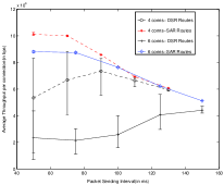
(a) Throughput Study

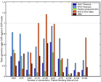
(b) Connection metrics

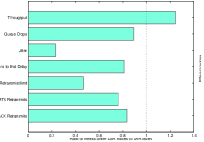
(c) Performance in Random Topology

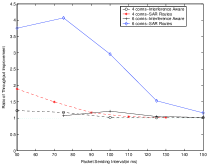
(d) Comparing to Interference Aware Routing

Figure 3: Performance of Scheduling-aware Routing(SAR)

Performance Evaluation of SAR: In this section, we evaluate the performance of SAR with standard routing schemes. A simple grid topology is first studied to illustrate the effect of the scheduling. The DSR routing protocol was used to compare the scheduling effectiveness. Since SAR uses static routes, and to provide a fair comparison, eliminating routing overhead and false disconnections, we allowed DSR to use static routes (selecting the most commonly used shortest path found by DSR).

A 4 and 6 connection scenario was analyzed in a 6$\times$6 grid topology. The sending rate was altered to observe the effects at various traffic loads. Figure 3(a) shows the throughput analysis. The error-bars indicate the variation of the throughput across different seeds. A performance improvement of around 4x and 2x was observed with 4 and 6 connections respectively. Note that under low sending rate (higher sending intervals), the scheduling effects play a less important role. Under high traffic loads, it can be observed that even the maximum throughput of the DSR routing scheme is significantly lesser than a scheduling aware routing scheme. Figure 3(b) shows the ratio of various connection metrics for SAR compared to the idealized DSR routes. A pronounced improvement was found in the majority of the metrics, especially the collision metrics like RTS Timeout, ACK Timeout and the packet drops due to retransmission limit. The ratio of standard routes’ connection metrics to the SAR metrics under a scenario of 8 random multi-hop connections in a random deployment of 144 nodes in a 1600m$\times$1600m area is shown in Figure 3(c).
Comparison with Interference Aware Routing: The effectiveness of the scheduling interactions was compared with Interference Aware Routing (IAR) schemes. Existing IAR schemes follow the Protocol Model  [2]. Figure 3(d) compares the ratio of the throughput of IAR and SAR to the counterpart standard routes under different sending rates. It was observed that under a reasonable traffic, IAR routes do not account for scheduling, and therefore perform significantly worse than SAR routes.

VI Concluding Remarks

In this paper, we first demonstrated that aggregate metrics of link capacity such as observed channel busy time are only effective in estimating the upper bound of link performance. Examination of low-level scheduling effects demonstrates that MAC interactions play a critical role in how interference is manifested. The key insight is that destructive behavior at the MAC level arises from sources that interfere but are not prevented from transmission by the MAC protocol. Thus, it is desirable to avoid links that experience mutually destructive interaction.

We used this observation to develop a methodology for ranking active links based on their interactions with other active links. Specifically, we identify the sets of sources that can transmit concurrently per the rules of the MAC protocol. With the exception of rare race conditions, collisions occur due to interactions within such sets. Based on an analysis of destructively interacting sources in independent sets, we develop an estimate for the expected RTS timeouts and expected ACK timeouts. We show that these estimates, which we call Interference Based Link Rating (IBLR) correlate strongly with observed packet drops. We demonstrate the effectiveness of IBLR rating by using them in a linear programming formulation of traffic engineering in static MHWNs. We show that capturing the scheduling effects leads to considerable improvement in performance of the derived routes, even for the small size scenarios we considered. If these results can transition to realistic environments, they have important implications for mesh network traffic engineering and provisioning. Further, identifying the nature of collisions that influence the quality of the links provides a starting point for distributed algorithms that capture these interactions in a distributed environment.

References

- [1] P. Gupta and P. Kumar, “The Capacity of Wireless Networks,” in IEEE TRANSACTIONS ON INFORMATION THEORY, 2000.
- [2] K. Jain, J. Padhye, V. N. Padmanabhan, and L. Qiu, “Impact of interference on multi-hop wireless network performance,” in MobiCom, 2003.
- [3] M. Kodialam and T. Nandagopal, “The Effect of Interference on the Capacity of Multi-hop Wireless Networks,” in Bell Labs Technical Report, 2003.
- [4] V. Kolar and N. B. Abu-Ghazaleh, “A Multi-Commodity Flow Approach to Globally Aware Routing in Multi-Hop Wireless Networks,” in IEEE PerCom, 2006.
- [5] J. Li, C. Blake, D. S. J. D. Couto, H. I. Lee, and R. Morris, “Capacity of Ad Hoc wireless networks,” in MobiCom, 2001.
- [6] C. L. Barrett, M. Drozda, A. Marathe, and M. V. Marathe, “Analyzing interaction between network protocols, topology and traffic in wireless radio networks,” in IEEE WCNC, 2003.
- [7] M. Takai, J. Martin, and R. Bagrodia, “Effects of wireless physical layer modeling in mobile ad hoc networks,” in MobiHoc, 2001.
- [8] D. S. J. D. Couto, D. Aguayo, B. A. Chambers, , and R. Morris, “Performance of multihop wireless networks: Shortest path is not enough,” in HotNets-I, 2002.
- [9] A. Adya, P. Bahl, J. Padhye, A. Wolman, and L. Zhou, “A Multi-Radio Unification Protocol for IEEE 802.11 Wireless Networks,” in BroadNets, 2004.
- [10] D. S. J. D. Couto, D. Aguayo, J. Bicket, and R. Morris, “A high-throughput path metric for multi-hop wireless routing,” in MobiCom ’03, 2003.
- [11] R. Draves, J. Padhye, and B. Zill, “Comparison of routing metrics for static multi-hop wireless networks,” in SIGCOMM, 2004.
- [12] D. Ganesan, B. Krishnamachari, D. C. A. Woo, D. Estrin, and S. Wicker, “Complex behavior at scale: An experimental study of low-power wireless sensor networks,” in Tech. Report UCLA CSD-TR 02-0013, 2002.
- [13] A. Woo, T. Tong, and D. Culler, “Taming the underlying challenges of reliable multihop routing in sensor networks,” in SenSys ’03, 2003.
- [14] A. Cerpa, J. L. Wong, M. Potkonjak, and D. Estrin, “Temporal properties of low power wireless links: modeling and implications on multi-hop routing,” in MobiHoc ’05, 2005.
- [15] J. Padhye, S. Agarwal, V. N. Padmanabhan, and Lili, “Estimation of Link Interference in Static Multi-hop Wireless Networks,” in Internet Measurement Conference, 2005.
- [16] M. Garetto, T. Salonidis, and E. W. Knightly, “Modeling per-flow throughput and capturing starvation in CSMA multi-hop wireless networks,” in IEEE INFOCOM, 2006.
- [17] V. Bharghavan, A. Demers, S. Shenker, and L. Zhang, “MACAW: A Media Access Protocol for Wireless LANs,” in SIGCOMM, 1994.
- [18] K. Xu, M. Gerla, and S. Bae, “How Effective is the IEEE 802.11 RTS/CTS Handshake in Ad Hoc Networks?” in Globecom, 2002.
- [19] J. W. Moon and L. Moser, “On cliques in graphs,” in Israel Journal of Mathematics, 1965.
- [20] “Qualnet network simulator, version 3.6,” http://www.scalable-networks.com/.
- [21] A. Nasipuri, R. Castaneda, and S. R. Das, “Performance of multipath routing for on-demand protocols in mobile adhoc networks,” Mob. Netw. Appl., vol. 6, no. 4, pp. 339–349, 2001.