JiTS: Just-in-Time Scheduling for Real-Time Sensor Data Dissemination

Abstract

We consider the problem of real-time data dissemination in wireless sensor networks, in which data are associated with deadlines and it is desired for data to reach the sink(s) by their deadlines. To this end, existing real-time data dissemination work have developed packet scheduling schemes that prioritize packets according to their deadlines. In this paper, we first demonstrate that not only the scheduling discipline but also the routing protocol has a significant impact on the success of real-time sensor data dissemination. We show that the shortest path routing using the minimum number of hops leads to considerably better performance than Geographical Forwarding, which has often been used in existing real-time data dissemination work. We also observe that packet prioritization by itself is not enough for real-time data dissemination, since many high priority packets may simultaneously contend for network resources, deteriorating the network performance. Instead, real-time packets could be judiciously delayed to avoid severe contention as long as their deadlines can be met. Based on this observation, we propose a Just-in-Time Scheduling (JiTS) algorithm for scheduling data transmissions to alleviate the shortcomings of the existing solutions. We explore several policies for non-uniformly delaying data at different intermediate nodes to account for the higher expected contention as the packet gets closer to the sink(s). By an extensive simulation study, we demonstrate that JiTS can significantly improve the deadline miss ratio and packet drop ratio compared to existing approaches in various situations. Notably, JiTS improves the performance requiring neither lower layer support nor synchronization among the sensor nodes.

1 Introduction

Wireless sensor networks are an important emerging technology that will revolutionize sensing for a wide range of scientific, military, industrial and civilian applications. A large number of inexpensive sensors collaborating on sensing a phenomena provide cost-effect detailed monitoring of the area under observation. While some sensor networks are deployed to collect information for later analysis, most applications require monitoring or tracking of phenomena in real-time. A primary challenge in such applications is how to carry out sensor data dissemination given source-to-sink end-to-end deadlines when the communication resources are scarce. The bursty nature of traffic in sensor networks, as the degree of observed activity varies, can cause the network resources to be exceeded. Moreover, the ad hoc nature of multi-hop sensor networks makes it difficult to schedule network traffic centrally as in traditional real-time applications.

Existing solutions for real-time data dissemination [1] prioritize packet transmission at the MAC layer according to the deadline and distance to the sink. These work have several limitations, including: (1) While packets are prioritized, they are not delayed. When traffic is bursty, high contention may result, increasing transmission and queuing delays. Further, packets generated by different sensors at the same time (e.g., in response to a detected event), can lead to high collision rates. (2) MAC level solutions cannot account for the queuing delay in the routing layer (occurring above the MAC layer) that has a significant impact on end-to-end delay especially under high load; and (3) MAC level solutions require re-engineering of the sensor radio hardware and firmware, making deployment difficult and potentially causing interoperability problems with hardware supporting different MAC protocols. In addition to these effects, the role of the routing protocol in the real-time scheduling success is not sufficiently examined. Geographical Forwarding, used in [1, 2, 3, 4], does not always use the shortest path, making it more difficult to meet the deadline. Furthermore, using a longer path causes the contention for the transmission medium to increase as more transmissions are needed to reach the sink. (An overview of the related work is presented in Section 2.)

The primary contribution of this paper is a new Just-in-Time Scheduling (JiTS) approach for real-time data dissemination in sensor networks that addresses many of the shortcomings of the existing solutions. JiTS delays packets at every hop for a duration of time which is a function of distance to the sink and the deadline. JiTS uses an estimate of the MAC layer transmission delay and accounts for it when deciding how long to delay a packet. By delaying the packets, rather than only prioritizing them, JiTS achieves the following advantages: (1) A full estimate of the delay is used, including the queuing delay at the network layer; (2) The load is distributed over the available slack time, potentially allowing the network to tolerate transient periods of high contention gracefully and to avoid transient hot-spotting; and (3) It provides packets with a longer time to wait for correlated packets for aggregation or packet combining. (In this paper, we do not pursue the aggregation effect, but reserve it for future work.)

The base JiTS algorithm distributes the slack time (available time before the deadline expires) uniformly across hops. However, in a data collection application, the degree of contention is typically higher closer to the sink. Therefore, a second contribution of this paper is to explore policies that allocate the time non-uniformly among the hops, to provide more slack time for transmission to the hops closer to the sink; we call this version of the algorithm JiTS with non-linear delays (JiTS-NL). The third contribution of the paper is to show that Shortest Path routing outperforms Geographical Routing with respect to real-time traffic. The design of JiTS is discussed in detail in Section 3.

In Section 4, the performance of JiTS is compared to RAP [1] and SPEED [2] with different deadline constraints and routing protocols. JiTS outperforms RAP both in terms of deadline miss ratio and packet drop ratio. Further, the nonlinear delay version of JiTS is able to achieve the best performance. These results hold across different network topologies (regular and random), and different traffic conditions. In particular, when the traffic generation is bursty, JiTS performance far out-paces that of RAP. JiTS also performs much better than SPEED, especially under high load scenarios. Finally, in Section 5, we conclude the paper and discuss future work.

2 Related work

Lu et al. [1] propose a real-time communication architecture in sensor networks, called RAP, which is most relevant to our work. They propose a Velocity Monotonic Scheduling (VMS) algorithm to prioritize the data packets. VMS derives the required packet “velocity”, which serves as its priority, from the deadline and distance between source and sink. In Static VMS, the velocity is computed once at the source. Conversely, in Dynamic VMS velocity is recomputed at intermediate nodes. Three queues are used for scheduling packets, where a packet falling in one of the three different priority levels is queued into the corresponding queue in a FIFO manner, with fixed priority enforced among the queues. It also modifies the MAC layer back-off scheme to schedule packets according to priority.

The SPEED framework [2, 3] proposes an optimized Geographic Forwarding routing for sensor network. To provide soft real-time guarantees, SPEED uses a MAC layer estimate of one-hop transmission delay to select the next hop to forward the data packet to. However, SPEED does not delay the packets via scheduling or prioritize data packets.

Li et al. [5] prove that scheduling parallel messages with deadlines over a wireless channel is NP-hard. They propose Last Start Time First (LSTF) scheduling which schedules messages based on per-hop timeliness constraints by manipulating MAC layer back-offs. They also study the spatial reuse of the wireless channel and the effect of collision avoidance.

Multi-hop coordination priority scheduling [6] proposed to incorporate the distributed priority scheduling into existing IEEE 802.11 priority back-off schemes to approximate an ideal schedule. The proposed multi-hop coordination scheduling allows the downstream nodes to increase a packet’s relative priority to make up for excessive delays incurred upstream. The scheduling requires modifications of the MAC layer, while possibly overloading the network.

Generally, the ability to meet real-time deadlines in the presence of contention is related to controlling the load presented to the system. In terms of networking resources, a related problem is that of congestion control. The importance of congestion control in sensor networks was identified [7] and approaches for addressing it have been developed [8]. Kang et al. study the possibility of addressing congestion by using multiple paths [9]. Exploring the intersection of congestion control and real-time scheduling is a topic of future research.

SWAN [10] is a stateless network model differentiating the service between real-time and best-effort traffic in wireless ad hoc networks. It supports per-hop and end-to-end control algorithms without per-flow information. SWAN uses local rate control for UDP and TCP best-effort traffic and sender-based admission control for real-time UDP traffic. Explicit congestion notification is used to dynamically regulate admitted real-time sessions in the face of network dynamics due to mobility or traffic overload conditions. SWAN and other QoS management schemes in wireless ad hoc networks usually support unicast network traffic;therefore, they do not map to many-to-one data dissemination operations prevalent in sensor networks.

3 Just-in-Time Scheduling Framework

We consider real-time data dissemination in sensor network applications where sensor data is being gathered to a sink. The effectiveness of the dissemination can be measured in terms of the deadline miss ratio (indicating how many packets miss their deadlines) and the packet drop ratio (indicating how many packets are dropped before arriving at the sink). The performance is affected by both the routing protocol and the packet scheduling algorithm. Consider that in the absence of contention, the delay of a packet is proportional to the number of hops on the path from the sensor to the sink, where the selected path is determined by the routing protocol. In the presence of contention, additional delays are incurred as the packets are queued behind other packets. Also, data transmission can take longer as the wireless channel is more highly utilized.

In this section, we describe the proposed Just-in-Time Scheduling algorithm (JiTS). We first discuss the role of the routing protocol and the two routing protocols that we use in Section 3.1. Section 3.2 then presents the scheduling algorithms of JiTS and compares them to those of RAP.

3.1 Routing Protocols

Existing real-time sensor network protocols, such as the RAP [1] and SPEED [2, 3] rely on Geographical Forwarding (GF) as the routing protocol [11, 12, 13]. In these protocol, each node tracks the location of its one hop neighbors via GPS or some localization algorithm (e.g., [14]). Sensors know the geographical location of the sink, for example, via the dissemination of the periodic routing flood from the sink. Forwarding is accomplished by sending the data to the neighbor who is closest to the sink. The advantage of this approach is small routing overhead; that is, each node simply needs to track the location information of its neighbors. However, this approach may not yield the shortest path in terms of number of hops, and delivery is not guaranteed. Either RAP or SPEED cannot resolve the scheduling for a system based on GFG [11] or GPSR [12] since they are based on the distance progress which the face forwarding does not provide. In addition, GPS units are expensive and energy consuming, while localization algorithms introduce localization errors that may affect the routing effectiveness. Therefore, we investigate a Shortest Path (SP) routing protocol to illustrate the role that routing plays in determining the success of a real-time scheduling algorithm. Like GF, SP operates by having the sink periodically flood a packet advertising its presence in the network. Nodes set up their routing entries as they receive these advertisement messages, remembering the route with the shortest path to the sink and the network distance in number of hops.

JiTS requires knowledge of the distance to the sink and the End-to-end Estimate of the Transmission Delay (EETD) needed by the MAC layer to transmit a packet. The first piece of information is typically present in any traditional routing protocol such as SP or GF. The second piece of information (EETD) can also be collected by the routing layer. At every hop, we estimate the local Estimated Transmission Delay (ETD) by exchanging a packet infrequently with the next hop neighbor towards the sink. A more precise estimate of ETD requires MAC layer support [3]; however, we do not use this approach because it requires MAC layer changes.

Summing the ETDs of a data packet hop by hop is costly and may lead to inaccurate estimates since one hop ETD can fluctuate significantly. Therefore, we use the following function to decide the EETD:

$$EETD=ETD\cdot\frac{E2E~{}distance}{One~{}hop~{}distance}$$

where the distance can be measured in different ways. Since the queuing delay dominates the end to end delay mostly in a heavy traffic environment, a precise EETD is not necessary.

3.2 Just-in-Time Scheduling (JiTS)

Scheduling is the primary mechanism available to intermediate nodes achieve their deadlines. Existing approaches to real-time data dissemination in sensor networks attempt to prioritize packets according to deadline, but do not intentionally delay packets. In contrast, the proposed Just-in-Time Scheduling (JiTS) approach sets target transmission times for the packets in accordance with their deadline and the remaining distance along the path. As a result, (1) JiTS can achieve more effective dissemination by judiciously allocating the slack time (time until the deadline) among the intermediate hops; (2) JiTS can better handle bursty traffic by decreasing the chances of collisions; and (3) More data aggregation is possible as discussed before. In the remainder of this section, we describe JiTS in a stepwise manner.

3.2.1 JiTS Organization

In JiTS, each node must decide how long to delay a packet, while leaving it with sufficient time to meet the deadline. The time taken by a packet from the source to the sink could be divided into two parts: lower layers transmission delay spent for transmission below the network layer and queuing delay needed for routing-layer queuing at any intermediate node. We use the EETD estimate to approximate the MAC layer transmission delay. Since this time is spent below the network layer, the scheduling cannot directly affect it. The second component is the queuing delay: how long the packet is queued in the network layer before it is handed to the MAC layer for transmission. This delay can be directly controlled by the JiTS scheduler.

Figure 1: JiTS Organization

Figure1 shows the organization of JiTS. We assume that the deadline information for a packet is present in (or derivable from) it. It is possible that the slack time (available time until the deadline) is smaller than the remaining EETD. Since JiTS is mainly designed for soft real-time applications, JiTS immediately forwards such packets without any delay even if the packet misses the deadline.

The JiTS scheduler uses a single priority queue for packet forwarding based on the computed target transmission time. Transmission is accomplished via a timer that is set to the target transmission time of the head of the queue. When the queue is full, the JiTS scheduler selects the packet at the head of the queue to immediately forward it instead of dropping any packet in the queue.

3.2.2 Just-in-Time Scheduling Policies

Different JiTS scheduling policies can be developed based on the ways of allocating the available slack time among the intermediate nodes. In the basic JiTS algorithm, the target transmission time is set to be equal at all intermediate hops and is determined as follows:

$$Target~{}Delay=\dfrac{Deadline-EETD}{Distance(X,sink)}\cdot\alpha$$ (1)

where $Deadline$ is the end-to-end deadline between a source and sink and $\alpha$ is a constant ”safety” factor used to ensure that the real-time deadline would be met. When $\alpha=0.7$, for example, the target delay of the packet will be set to 0.7 times the available slack time, leaving the remaining time as a safety margin. For different JiTS policies, node $X$ means differently.

As we can see, the Target Delay of any in-queue packet determines its priority. The time a packet is delayed in the queue can be used as the key to a priority queue that holds the packets to be transmitted. The end-to-end transmission and processing delay is considered along with the queuing delay, by taking into account the end-to-end deadline, distance and EETD.

We consider the following policies for Just-in-Time Scheduling.

1. Static JiTS (JiTS-S): In JiTS-S, the target delay is set at the data source. In Equation 1, the end-to-end deadline is fixed at the data source; the EETD is measured with the ETD of forwarding node and the distance from source to sink ($X$ is the data source). Thus, even we call it static, the different ETD’s of forwarding nodes would make the target delay at each node different.

2. Dynamic JiTS (JiTS-D): In JiTS-D, the target delay is reset at each forwarding node with the local value of parameters. In Equation1, the end-to-end deadline of a packet at some forwarding node is the remaining slack time, measured by $Deadline-Elapsed~{}Time$. The EETD is decided by the one-hop ETD of the forwarding node and the distance from it to the sink, but not by the distance from the source to sink ($X$ is the current forwarding node). Hence, the dynamic JiTS is able to continuously refine the priority of the packet.

3. Non-linear JiTS (JiTS-NL): It is also possible to allocate the available slack time non-uniformly among the intermediate hops along the path to the sink. For example, we may desire to provide the packets with additional time as it goes closer to the sink. The intuition is that in a gathering application, the contention is higher as the packet moves closer to the sink. Different policies can be developed to break down the available time.

We explore the following policy for JiTS-NL:

$$Target~{}Delay=\dfrac{Deadline-EETD}{2^{R/O}}\cdot\alpha$$ (2)

where $R$ and $O$ are the remaining distance to the sink and one hop distance, respectively. More generally, it is desired to allocate the slack time proportionately to the degree of contention along the path. Such a heuristic may be developed by passing the contention information along with the routing advertisement and allocating the available slack time accordingly. A thorough investigation is reserved as future work.

3.2.3 Just-in-Time Scheduling for Different Routing Protocols

JiTS can be adapted to work with virtually any underlying routing protocol. However, the JiTS algorithm may need to be adapted to consider the cost metric used by the routing algorithm. For example, in a system based on the shortest path routing (SP), the distance parameters used by JiTS scheduler is measured in number of hops. The corresponding functions for basic JiTS (Equation 1) and non-liner JiTS (Equation 2) are as follows:

$$Target~{}Delay=\dfrac{Deadline-EETD}{h}\cdot\alpha$$ (3)

$$Target~{}Delay=\dfrac{Deadline-EETD}{2^{h}}\cdot\alpha$$ (4)

where $EETD=ETD\cdot h$ and $h$ stands for the end-to-end number of hops. (For the geometric routing, the values of distance parameters used in JiTS scheduler is the Euclidean distance.)

In summary, the following information is needed to schedule packets in JiTS:

• End-to-end deadline information: This information is provided by the application as part of the data packet to meet the requirements of the specific real-time data dissemination application.

• End-to-end distance information: this information is obtained from the routing protocol. For example, this information is maintained in the routing tables of traditional distance vector based or link-state based routing protocols to keep track of the cost of the path. Furthermore, in source routed protocols such as DSR[15], this information can be directly computed from the packet header which includes the full path to the destination. Finally, in geographic routing, Euclidean distance measured as the distance from the current node to the destination can be used as the distance metric.

The output of JiTS scheduler is the queuing delay, which is used by the routing protocol to decide how long to delay an incoming data packet before attempting to forward it (by passing it to the MAC layer). MAC layer prioritization is not needed by the JiTS design, since a packet is sent when only its just-in-time local deadline, i.e., target delay, is reached. Thus, the MAC layer needs no change to use our JiTS algorithms.

If the traffic through the current node is not heavy and queuing time is more than enough for any packet with lenient deadline requirement, just-in-time scheduling (or any scheduling) is not needed and may end up harming performance. If such a situation can be detected, JiTS can be disabled and packets forwarded normally. For example, an idle detection mechanism may be employed such that if an idle period passes without packet transmission, the head of the queue is sent immediately.

4 Experiments

We implemented the Static, Dynamic and Non-Linear JiTS with both Shortest Path (SP) routing and Geographic Forwarding (GF) in the Network Simulator (NS2, version 2.27) [16]. We also implemented the RAP Velocity Monotonic Scheduling (VMS) with GF, including the specialized MAC support following the specification of the authors [1], as well as the SPEED protocol [2, 3]. Since GF has been shown to significantly outperform traditional routing protocols, such as DSR [15], in sensor network data dissemination, we restrict the routing comparison to GF and SP.

4.1 Comparisons with VMS

Table 1 shows the simulation parameters we use to compare JiTS to Velocity Monotonic Scheduling (VMS) adopted by RAP [1]. Unless otherwise indicated, these parameters are used in this studies.

MAC protocol	IEEE 802.11
Transmission Range	250 m
Bandwidth	2Mbps
Data Packet Size	32B
Data Rate	2 packet/s
Routing Period	5 s
Simulation Area	1000 $\times$ 1000 $m^{2}$
Sensor Nodes	100
Simulation time	120 s

Table 1: Simulation parameters

We use scenarios with 100 sensors and investigate both $10\times 10$ grid and random deployment. In the grid scenarios, the sink is placed on the northwest corner of the network. In random deployment, the 100 nodes are randomly placed in the simulation area while the sink is placed roughly at the center of the area.

We compared JiTS scheduling with the VMS both using the same routing protocol (GF) that was used in the original RAP scheme [1]. Later, we also show that SP significantly outperforms GF for JiTS. As discussed before, we use soft-deadline policy for all protocols where packets are not dropped if their deadline is exceeded. We note that a hard deadline version of JiTS could be easily developed; however, we conjecture that soft-deadlines are likely to be a more realistic model for sensor networks. Since JiTS does not require any MAC layer information, we use the original IEEE 802.11 as our MAC layer protocol, while we use the modified MAC layer for RAP as done in [1]. We have implemented Static, Dynamic and Nonlinear JiTS policies and compared their performance with RAP.

We considered the issue of what the JiTS safety margin parameter $\alpha$ should be set to. If $\alpha$ is too high, most of the slack time is taken up by the intentional JiTS delay. As a result, additional unexpected delays, if any, may cause a packet deadline miss. Conversely, if the $\alpha$ is too low, packets are conservatively sent quickly towards the sink, possibly overflowing buffers around it. Experimentally, we observed that a safety margin parameter of 0.7 works well across different deadlines. Thus, 30% of the slack time is set aside to account for unexpected transmission or queuing delays. (An analytic derivation of $\alpha$ is reserved for future work.)

4.1.1 Evaluation of JiTS and VMS

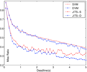
Figure 2: JiTS(GF) vs VMS Miss Ratio

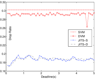
Figure 3: Drop Ratio: JiTS(GF) vs VMS

The first experiment compares the performance of JiTS to RAP. Figure 2 and figure 3 show that for different deadline requirements, the miss ratios of Static and Dynamic JiTS are much lower than those of Dynamic VMS(DVM) and Static VMS(SVM) across all the tested deadlines. The same observation holds for the drop ratios. Dynamic JiTS outperforms static JiTS in terms of the miss ratio.

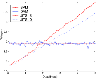
Figure 4: Average Delay: JiTS (GF) vs VMS

Figure 4 shows the average delay of JiTS and RAP to illustrate the difference between the two scheduling approaches. The average delay of JiTS grows linearly with the deadline as the intermediate nodes delay packets proportionately to the deadline. In this way, we can take advantage of the slack under overload. Note that dynamic JiTS manages to keep the average delay around the value of $0.7\cdot deadline$, while the static JiTS has slightly higher average delay. Since RAP does not delay packets, its delay only depends on the data generation pattern and does not change with the deadline.

Since the VMS uses multiple FIFO queues as its priority queue, packet starvation commonly happens and the maximum packet delay suffered by RAP is much worse than that of JiTS by a factor of 2 to 3. (Due to space limitations, we do not include the results here.) We will only compare our JiTS policies with SVM in the remainder of this paper, because the performance of SVM and DVM is similar and the authors of RAP observed SVM to be superior to DVM [1].

4.1.2 Effect of Routing Protocol

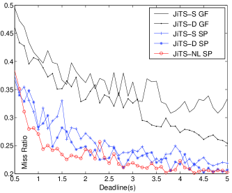
Figure 5: JiTS SP vs GF Miss Ratio

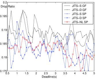
Figure 6: Drop Ratio: JiTS SP vs GF

In the second set of experiments, we compare the performance of JiTS under GF with JiTS with Shortest Path (SP) routing. In addition, in this experiment, we include the performance of the nonlinear JiTS scheduling algorithm (JiTS-NL). Figure 5 and Figure 6 show the miss ratio and drop ratio respectively. From these figures, we observe that JiTS performs considerably better with SP than with GF. In general, dynamic JiTS performs better than static JiTS for both routing protocols. Furthermore, JiTS-NL provides significant improvements compared to static and dynamic JiTS. Especially, the improvement is most pronounced under tight deadlines showing the applicability of JiTS-NL to real-time data dissemination. The maximum and average delay of JiTS with GF is higher than that with SP for the same deadlines (results not shown) because GF may use longer paths than SP in terms of the number of hops.

4.1.3 Performance under Bursty Traffic

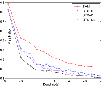
Figure 7: Miss Ratio of Bursty: JiTS vs SVM

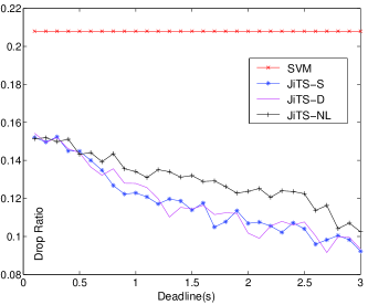
Figure 8: Drop Ratio of Bursty: JiTS vs SVM

In this set of experiments, we evaluate the performance of JiTS vs. RAP under bursty traffic conditions. At every 10 seconds we let all the nodes publish data packets with the pre-set data rate in the first 5 seconds then stop publishing for the remaining 5 seconds. Figures 7 and 8 show the miss ratios and drop ratios of JiTS and SVM under bursty traffic with end-to-end deadline increasing from 0.1 second to 3.0 seconds. In Figure 7, we can see that the miss ratio of dynamic JiTS is much lower than that of SVM under the bursty traffic, because JiTS can tolerate the traffic burst by delaying some packets, and taking advantage of the idle period. On the other hand, SVM cannot make use of the traffic behavior, since it does not delay packets even if there is slack. In Figure 8, we observe that JiTS disciplines achieve the lower the drop ratios than SVM, delivering more packets as the deadline constraints are relaxed. In contrast, SVM suffers almost the same drop ratio even when the deadlines are relaxed.

4.1.4 Performance under Random Deployment

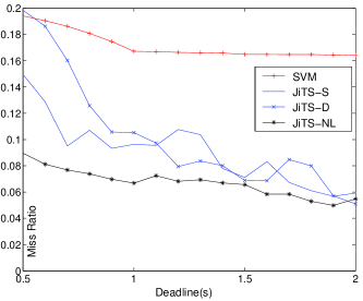
Figure 9: Random Scen. Miss Ratio (GF)

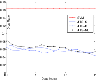
Figure 10: Random Scen. Drop Ratio (GF)

JiTS and SVM were also evaluated using constant traffic (Table 1) and a random deployment scenario where the 100 nodes were randomly placed within the simulation area. To be fair, we associate JiTS with GF routing which SVM is based on. We varied the deadline requirements from 0.5 to 2.0 seconds in steps of 0.1 seconds. Figures 9 and 10 show the miss ratios and drop ratios of the tested algorithms. The simulations show that both JiTS and SVM perform much better in a random scenarios than they did in the grid scenarios possibly because the location of the sink is central to the simulation area, making the average sensor distance to the sink smaller. Again JiTS provides superior performance to SVM. For the SVM, the drop ratios do not decrease as the deadline grows since it prioritizes but does not delay packets as shown in Figure 10. The drop ratio becomes the lower bound of the miss ratio. JiTS shows more reactivity in that both the drop ratio and miss ratio decrease as the deadline requirement is relaxed.

4.1.5 Performance with Multiple Deadline Data

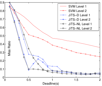
Figure 11: Two Level Deadlines: Miss Ratio

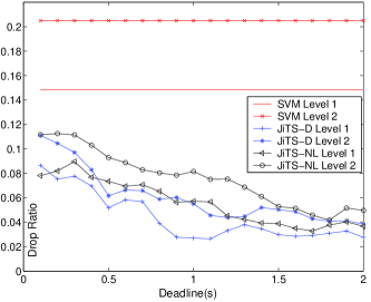
Figure 12: Two Level Deadlines: Drop Ratio

We simulated the presence of two data types being generated by the sensors with two different deadline constraints (deadline of level 1 data is half that of level 2 data), in bursts. Ideally, the scheduling algorithm would allow both data types to meet their deadlines effectively. Figures 11 and 12 show the miss ratio and drop ratio of SVM, JiTS Dynamic and Non-Linear. Under strict deadlines, level 2 traffic receives better performance, because the network was often unable to satisfy the aggressive level 1 deadlines. Once the deadlines increase beyond a certain level, JiTS is able to provide similar performance to the two traffic types, despite the different deadline requirements. However, the same is not true of SVM, where level 2 traffic continues to receive better performance than level 1 traffic.

4.2 Comparisons with SPEED

We also built simulation models for the SPEED framework [2, 3] within the NS-2 simulator. We implemented the full specification of SPEED, SPEED-T (Minimal one hop delay first), and SPEED-S (maximal one hop progress speed first). For validation, we first repeated the experiments conducted in the original SPEED paper [2]. We note that the original SPEED implementation was built in a different simulator (GloMoSim [17]) which has different wireless models than NS-2. Further, the authors did not specify exact values of the several (at least four) simulation parameters that they used in their experiments. (In a personal communication with one of the authors, he indicated that the parameters were manually tuned for each case and we were not able to repeat the exact configuration.) Nevertheless, our obtained results were very close to those achieved by the original paper (but not identical). In this section, we first compare the performance of SPEED with GF and SP and then compare SPEED with JiTS under different traffic load levels.

4.2.1 Evaluation of SPEED and routing protocols

We compared the simulation results against the shortest-path routing and geographical forwarding routing in a void-free deployment. In this study, all the data flows are constant, while some congestion-introducing flows are created in some intermediate nodes in the same manner used in the original SPEED design[2, 3].

Figure 13 and Figure 14 show the performance of SPEED.

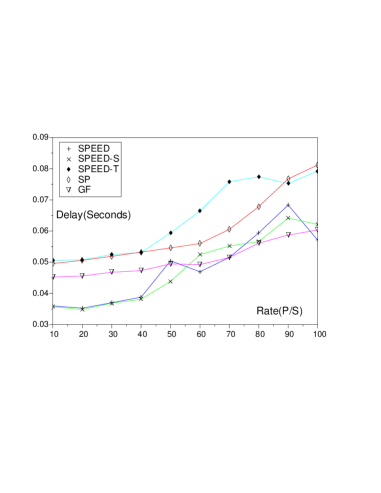
Figure 13: SPEED: end-to-end delay

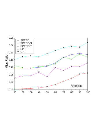
Figure 14: SPEED: miss ratio

For the congestion-introducing flow with lower data rate, SPEED and GF perform similarly as observed in the original SPEED paper[2]. In terms of end-to-end delay, SPEED is better than both the GF and SP in most cases, especially when the data rate of congestion-introducing flow is low. However, the miss ratio of SPEED becomes higher than GF and SP in all cases. It is very high even when the data rate of congestion-introducing flow is low. The miss ratios of GF and SP are not as high as the values reported in [2]. The possible reason of it is that the SPEED tries to drop some data packets when “SPEED” can not be maintained in some intermediate nodes, which would backpressure the data source. The future dropping possibility would be increased as this situation keeps happening. Meanwhile, neither GF or SP in our simulation drop data packets (in the routing layer), leading to a lower drop ratio.

Figure 15 shows the drop ratio of SPEED against both the GF and SP. The drop ratio of SPEED is much higher than that of SP. It is also a little bit higher than GF. As we can see, the high miss ratio mostly results from SPEED’s high drop ratio. As expected, SP outperforms GF. Since the drop ratio of SP is much lower than the GF, it seems that more data packets with longer end-to-end delay are received by SP, which leads to the higher average end-to-end delay as shown in Figure13.

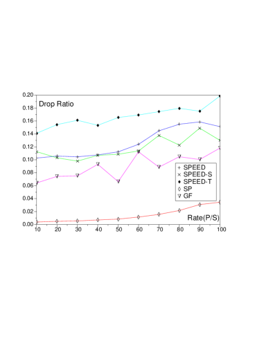
Figure 15: SPEED: drop ratio

Figure 16 shows the average number of hops from source to sink. The average hops of SP is the lowest in all, since it provides the shortest path at any time. GF also uses shorter paths than SPEED. This is mainly because SPEED does not always try to minimize the number of hops or select the geographically closest neighbor.

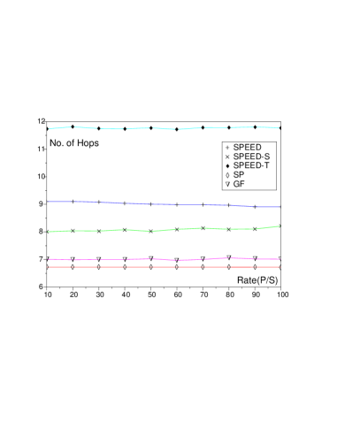
Figure 16: SPEED: average hops

4.2.2 Evaluation of JiTS and SPEED

In this subsection, we SPEED with JiTS under different traffic load levels. Specifically, we use three different traffic load levels in a 10 by 10 grid deployment. Load I and Load II have 100 sources generating packets at 1 packet/sec and 0.5 packet/sec respectively. In case Load III, there are 10 sources generating packets at 1 packet/sec.

Figure 17 and figure 18 show their miss ratios and drop ratios of JiTS and SPEED under the three different traffic levels. Under medium and high traffic load, the drop ratios and miss ratios of SPEED are very high as SPEED attempts unsuccessfully to route around congestion. In contrast, JiTS adapts with different levels of traffic loads. In light traffic, the two approaches perform comparably.

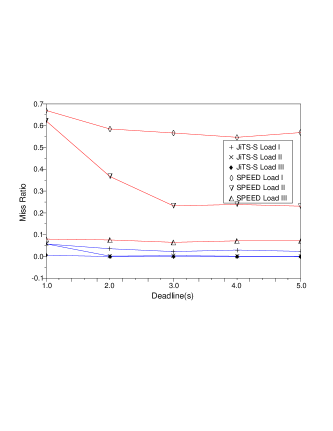
Figure 17: JiTS vs SPEED: Miss Ratio

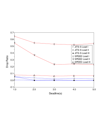
Figure 18: JiTS vs SPEED: Drop Ratio

Figure 19 shows the average number of end-to-end hops of all received data packets. Since JiTS uses SP as basic routing, the average number of hops is kept stable. SPEED has a higher average number of hops due to the backpressure mechanism. If the timing constraint becomes more stringent, SPEED seems to drop more packets at intermediate nodes, statistically reducing the average number of hops traveled by the delivered packets.

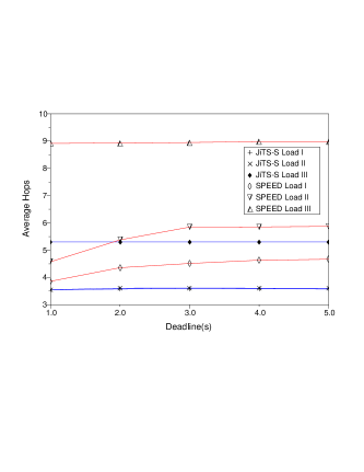
Figure 19: JiTS vs SPEED: Average Hops

5 Conclusions and Future Work

Real-time data dissemination is a service of great interest to many sensor network applications. We proposed and evaluated the Just-in-Time scheduling mechanisms for the real-time sensor networks applications that offers significant advantages over existing real-time sensor data dissemination schemes. JiTS accomplishes real-time support by delaying packets a fraction of their slack time at each hop. As a result, it is better able to tolerate bursts than schemes that simply prioritize packet transmission. We also explored the effect of routing on real-time scheduling success and showed that Geographical Forwarding can lead to suboptimal operation. JiTS outperforms RAP in both the miss ratio and overall delay. We explored several criteria for allocating the available slack time among the different nodes and showed that nonlinear distribution of the slack time, assigning more time assessed to hops closer to the sink, results in better performance than linear distribution of the slack time. Further, JiTS is a routing layer solution and does not require changes to lower level protocols. As a result, it can be deployed independent of the underlying sensor network hardware capabilities. From the simulations, we found the drop ratio is the lower bound of the miss ratio of real-time communication. If the drop ratio is decreased, given a reasonable end-to-end deadline, the miss ratio of these real-time applications should also be decreased. Mostly the packets are dropped due to congestion as the network capacity is exceeded. In the future, we will further investigate JiTS in the context of wireless sensor networks. We will also investigate other related issues such as data aggregation in JiTS and congestion control for real-time data transmission in sensor networks.

References

- [1] Chenyang Lu, Brian M. Blum, Tarek F. Abdelzaher, John A. Stankovic, and Tian He. RAP: A real-time communication architecture for large-scale wireless sensor networks. RTAS’02, 2002.
- [2] Tian He, John A Stankovic, Chenyang Lu, and Tarek Abdelzaher. SPEED: A stateless protocol for real-time communication in sensor networks. ICDCS’03, 2003.
- [3] Tian He, John A. Stankovic, Chenyang Lu, and Tarek F. Abdelzaher. A spatiotemporal protocol for wireless sensor network. IEEE Transactions on Parallel and Distributed Systems, 2005.
- [4] Emad Felemban, Chang-Gun Lee, Eylem Ekici, Ryan Boder, and Serdar Vural. Probabilistic QoS guarantee in reliability and timeliness domains in wireless sensor networks. IEEE INFOCOM’05, 2005.
- [5] Huan Li, Prashant Shenoy, and Krithi Ramamritham. Scheduling messages with deadlines in multi-hop real-time sensor networks. UMASS CMPSCI Technical Report TR04-91, 2004.
- [6] V. Kanodia, C. Li, A. Sabharwal, B. Sadeghi, and E. Knightly. Distributed multi-hop scheduling and medium access with delay and throughput constraints. MobiCom’01, 2001.
- [7] S. Tilak, N. Abu-Ghazaleh, and W. Heinzleman. Infrastructure tradeoffs in sensor networks. In WSNA’02, 2002. Held in Conjunction with MobiCom 2002.
- [8] Chieh-Yih Wan, Shane B. Eisenman, and Andrew T. Campbell. Coda: Congestion detection and avoidance in sensor networks. In SenSys’03, 2003.
- [9] JaeWon Kang and Yanyong Zhang and Badri Nath. Adaptive Resource Control Scheme to Alleviate Congestion in Sensor Networks. In Proc. of the First Workshop on Broadband Advanced Sensor Networks, 2004.
- [10] Gahng-Seop Ahn, Andrew T. Campbell, Andras Veres, and Li-Hsiang Sun. Supporting service differentiation for real-time and best effort traffic in stateless wireless ad hoc networks (SWAN). IEEE Transactions on Mobile Computing, 2002.
- [11] Prosenjit Bose, Pat Morin, Ivan Stojmenovic, and Jorge Urrutia. Routing with guaranteed delivery in ad hoc wireless networks. In 3rd ACM Int. Workshop on Discrete Algorithms and Methods for Mobile Computing and Communications DIAL M99, Seattle, WA, August 1999.
- [12] B. Karp and Kung. H. T. GPSR: Greedy perimeter stateless routing for wireless networks. MobiCom’00, 2000.
- [13] Guoliang Xing, Chenyang Lu, Robert Pless, and Qingfeng Huang. On greedy geographic routing algorithms in sensing-covered networks. MobiHoc’04, 2004.
- [14] N. Bulusu, J. Heidemann, and D. Estrin. GPS-less low cost outdoor localization for very small devices. IEEE Personal Communications Magazine, pages 28–34, October 2000.
- [15] David B. Johnson, David A. Maltz, and Josh Broch. DSR: The dynamic source routing protocol for multi-hop wireless ad hoc networks. In Charles E. Perkins, editor, Ad Hoc Networking, pages 139–172. Addison-Wesley, 2001.
- [16] The Network Simulator - ns-2. http://www.isi.edu/nsnam/ns/, 2005.
- [17] GloMoSim. http://pcl.cs.ucla.edu/projects/glomosim/.