Evolution of the Internet AS-Level Ecosystem

Abstract

We present an analytically tractable model of Internet evolution at the level of Autonomous Systems (ASs). We call our model the multiclass preferential attachment (MPA) model. As its name suggests, it is based on preferential attachment. All of its parameters are measurable from available Internet topology data. Given the estimated values of these parameters, our analytic results predict a definitive set of statistics characterizing the AS topology structure. These statistics are not part of the model formulation. The MPA model thus closes the “measure-model-validate-predict” loop, and provides further evidence that preferential attachment is a driving force behind Internet evolution.

I Introduction

The Internet is a paradigmatic example of a complex network. Many researchers have used publicly available data on Internet topology and its observed evolution to test a variety of physical models of complex network structure and dynamics. The large-scale Internet topology represent the structure of connections between companies owing parts of the Internet infrastructure, each company roughly corresponding to an Autonomous System (AS) Pastor-Satorras and Vespignani (2004). An AS might be a transit Internet service provider (ISP) or customer, a content provider or sink, or any combination of these. Some ASs span multiple continents and are highly interconnected, while others are present at a single geographical location and have only a few links. In 1999 Faloutsos et al. Faloutsos et al. (1999) observed that despite all this diversity, the distribution of AS degrees obeys a simple power law. This observation remains valid today, after ten years of Internet evolution Dhamdhere and Dovrolis (2008).

Many researchers have attempted to model the Internet as an evolving system Albert and Barabási (2000); Yook et al. (2002); Goh et al. (2002); Chang et al. (2003); Zhou and Mondragón (2004); Zhou (2006); Serrano et al. (2005, 2006); Chang et al. (2006); Wang and Loguinov (2006); D’Souza et al. (2007); Corbo et al. (2007); Bar et al. (2007); Holme et al. (2008), and have studied its properties Pastor-Satorras et al. (2001); Ravasz and Barabási (2003); Park and Newman (2003); Bianconi et al. (2005). However, questions regarding the main drivers behind Internet topology evolution remain Krioukov et al. (2007). In this paper our main objective is to create an evolutionary model of the AS-level Internet topology that simultaneously:

1. is realistic,

2. is parsimonious,

3. has all of its parameters measurable,

4. is analytically tractable, and

5. “closes the loop.”

Parsimony implies that the model should be as simple as possible, and, related to that, the number of its parameters should be as small as possible. The fifth requirement means that if we substitute measured values of these parameters into analytic expressions of the model, then these expressions will yield results matching empirical observations of the Internet. However, most critical is the third requirement Krioukov et al. (2007): as soon as a model has even a few unmeasurable parameters, one can freely tune them to match observations. Such parameter tweaking to fit the data may create an illusion that the model “closes the loop,” but in the end it inevitably diminishes the value of the model because there is no rigorous way to tell why one model of this sort is better than another since they all match observations. To the best of our knowledge, the multiclass preferential attachment (MPA) model that we propose and analyze in this paper is the first model satisfying all five requirements listed above.

A salient characteristic of our model is that we distinguish between two kinds of ASs: ISPs and non-ISPs. The main difference between these two types of ASs is that while both ISPs and non-ISPs can connect to ISPs, no new AS will connect to an existing non-ISP since the latter does not provide transit Internet connectivity. In Section II we analyze the effect of this distinction on the degree distribution. In Section III we account for other processes. ISPs can form peering links to exchange traffic bilaterally. They can also go bankrupt and be acquired by others. Finally, they can multihome, i.e., connect to multiple providers. Prior work has often focused on these processes as the driving forces behind Internet topology evolution. We show that in reality they have relatively little effect on the degree distribution. Using the best available Internet topology data, we measure the parameters reflecting all the process above, and analytically study how they affect the degree distribution.

However, the degree distribution alone does not fully capture the properties of the Internet AS graph Mahadevan et al. (2006a). The $dK$-series formalism introduced in Mahadevan et al. (2006a) defines a systematic basis of higher-order degree distributions/correlations. The first-order ($1K$) degree distribution reduces to a traditional degree distribution. The second-order ($2K$) distribution is the joint degree distribution, i.e., the correlation of degrees of connected nodes. The distributions can be further extended to account for higher-order correlations Mahadevan et al. (2006a), or for different types of nodes and links, called annotations Dimitropoulos et al. (2009). In the economic AS Internet, there are two types of links: links connecting customer ASs to their providers (customer-to-provider links), and links connecting ISPs to their peers (peer-to-peer links). Reproducing the $2K$-annotated distribution of AS topologies suffices to accurately capture virtually all important topology metrics Mahadevan et al. (2006a); Dimitropoulos et al. (2009). An important feature of the MPA model is that, by construction, it naturally annotates the links between ASs by their business relationships, and that we can analytically calculate, in Section IV, the distributions for the number of peers, customers, and providers that nodes have. In Section V we perform a $2K$-annotated test. We generate synthetic graphs using the MPA model, and find that these graphs exhibit a startling similarity to the observed AS topology according to almost all the $2K$-annotated statistics. This validation, in conjunction with observations in Mahadevan et al. (2006a); Dimitropoulos et al. (2009), ensures that other important topology metrics also match well.

II Two-Class Preferential Attachment Model

In the original preferential attachment (PA) model Barabási and Albert (1999), there is only one type of nodes. Suppose that nodes arrive in the system at the rate of one node per unit time, and let them be numbered $s=1,2,3,...$ as they arrive. Then the number of nodes in the system at time $t$ is equal to $t$. A node entering the system brings a link with it. One end of the link is already connected to the entering node, while the other end is loose. We call such an un-associated end a loose connection. According to the PA model, nodes attach to existing ones with a probability proportional to their degrees. Thus, the probability that a node of degree $k$ is selected as a target for the incoming loose connection, is its degree divided by the total number of existing connections in the system, which is $\frac{k}{2t}$. The original PA model yields a power-law degree distribution $P(k)\sim k^{-\gamma}$ with $\gamma=3$, but the linear preference function can be modified by an additive term such that the model produces power laws with any $\gamma>2$ Barabási and Albert (1999); Dorogovtsev et al. (2000); Krapivsky et al. (2000).

In the Internet, there are two fundamentally different types of ASs—ISPs and non-ISPs—that differ in whether they provide traffic carriage between the ASs they connect or not. No new AS would connect to an existing non-ISP since it cannot provide Internet connectivity. No other work has attempted to model this observation, which is fundamental to understanding the evolution of Internet AS-level topology. Thus, our first modification of the PA model is to consider these two classes of nodes (Figure 1). New ISPs appear at a rate $1$ and connect to other ISP-nodes with a linear preference. New non-ISPs appear at some rate $\rho$ per unit time, implying that the ratio $r$ of non-ISP nodes to the total number of nodes is

$$r=\frac{\rho}{1+\rho}.$$

Non-ISPs attach to existing ISP-nodes with a linear preference. However, no further attachments to non-ISPs can occur. Thus, with respect to degree distribution, only the ISP-nodes contribute to the tail of the power law as the non-ISP nodes will all have degree $1$. Given that a link between an ISP node and a non-ISP node has only one end that contributes to the degree of ISP nodes, and since we look only at ISP nodes to find the degree distribution, the links that have an ISP node on one end and a non-ISP node on the other should be counted only once, i.e., they are counted as contributing $1$ connection.

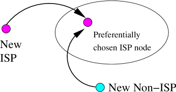
Figure 1: Two-class preferential attachment model. There are ISP nodes and non-ISP nodes.

Since each ISP node contributes $2$ connections to the network and a non-ISP node contributes only $1$, the total number of existing connections in the network at time $t$ is $(2+\rho)t$, which implies that the probability of any loose connection connecting to an ISP-node of degree $k$ is

$$\frac{k}{(2+\rho)t}.$$ (1)

We use the notation $p(k,s,t)$ to denote the probability that an ISP node $s$ has degree $k$ at time $t$. Then the average degree of an ISP node $s$ at time $t$ is

$$\bar{k}(s,t)=\sum_{k}kp(k,s,t)$$ (2)

Both entering ISPs and non-ISPs have one loose connection each, so the number of loose connections entering the system at time $t$ is $1+\rho$. Then, from (1), the continuous-time model of the system is

$$\frac{\partial\bar{k}(s,t)}{\partial t}=\frac{1+\rho}{(2+\rho)t}\bar{k}(s,t),$$ (3)

with boundary condition $\bar{k}(t,t)=1$ for $t>1$. Solving this equation yields

$$\bar{k}(s,t)=\left(\frac{s}{t}\right)^{-\frac{1+\rho}{2+\rho}}.$$ (4)

This model represents a deterministic system in which if ISP node $s$ has degree $\bar{k}$, then ISP nodes that arrived before $s$ (in the interval $[0,s)$) have degree at least $\bar{k}$. Thus, $s$ also represents the number of ISP nodes that have degree at least $\bar{k}$. It follows from (4) that the number of ISP nodes that have degree $\bar{k}$ or higher is

$$\frac{t}{\bar{k}^{\frac{2+\rho}{1+\rho}}}.$$

Note that the number of ISP nodes that arrive in $[0,t]$ is just $t$. Hence, the fraction of ISP nodes that have degree $\bar{k}$ or higher is

$$\frac{1}{\bar{k}^{\frac{2+\rho}{1+\rho}}}.$$

Since this fraction is essentially a complimentary cumulative distribution function (CCDF), we differentiate it and multiply by $-1$ to obtain the density function

$$f(\bar{k})=\frac{2+\rho}{1+\rho}{\bar{k}^{-\left(2+\frac{1}{1+\rho}\right)}},$$ (5)

which corresponds to the probability distribution

$$P(k)\sim k^{-\left(2+\frac{1}{1+\rho}\right)}=k^{-\left(3-r\right)}.$$ (6)

Validation Against Observed Topology 1

Dimitropoulos et al. Dimitropoulos et al. (2006) applied machine learning tools to the best available data from the Internet registry (WHOIS) and routing (Border Gateway Protocol (BGP)) systems to classify ASs into several different classes, such as Tier-1 ISPs, Tier-2 ISPs, Internet exchange points, universities, customer ASs, and so on. They validated the resulting taxonomy by direct examination of a large number of ASs. We use their results and divide ASs into two classes based on whether they are ISPs or not. According to Dimitropoulos et al. (2006) (the dataset is available at http://www.caida.org/data/active/as_taxonomy/), the number of ISPs is about $30\%$ of ASs, while non-ISPs make up the other $70\%$, i.e., $r=0.7$ and $\rho=7/3$. The measured value of $\rho$ yields $P(k)\sim k^{-2.3}$, with exponent close to the observed value between $-2.1$ and $-2.2$ Faloutsos et al. (1999); Chang et al. (2004); Mahadevan et al. (2006b).

The key point of this section is that the observed value of the power-law exponent close to $2$ finds a natural and simple explanation: it is due to preferential attachment and to a directly measured high proportion of non-ISP nodes to which newly appearing nodes cannot connect.

III Multiclass Preferential Attachment: Peering, Bankruptcy, Multihoming, and Geography

In this section we add further refinements to our model and show that, contrary to common beliefs, none of these refinements have a significant impact on the degree distribution shape.

Relationships between ASs change over time, as ASs pursue cost-saving measures. If the magnitude of traffic flow between two ISPs is similar in both directions, then reciprocal peering with each other allows each ISP to reduce its transit costs. Under the assumption that all customer ASs generate similar volumes of traffic, high degree ASs would exchange high traffic volume and rationally seek to establish reciprocal peering with other high degree ASs. We denote the rate at which peering links appear by $c$. The probability that a new peering link becomes attached to a pair of ISP-nodes of degree $k_{1}$ and $k_{2}$ is proportional to $k_{1}k_{2}$.

When ISPs go bankrupt, their infrastructure is usually acquired by another ISP, which then either merges the ASs or forms a “sibling” relationship in which their routing domains appear independent but are controlled by one umbrella organization. Thus, in terms of the topology, bankruptcy means that a connection shifts from one ISP to another. Since high degree ISPs tend to be wealthier, they are more likely to be involved in such takeovers. We denote the rate of bankruptcy by $\mu$ per unit time.

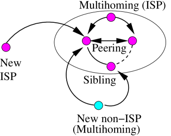
Figure 2: The multiclass preferential attachment model.

A growing AS may decide to multihome, i.e., to connect to at least two Internet providers. One would expect that higher degree ISPs with a need for reliability would multihome to other higher degree ISPs. We model this phenomenon by assuming that multihoming links appear in the system at rate $\nu$ per unit time. The probability that a new link becomes attached to a pair of ISP-nodes of degree $k_{1}$ and $k_{2}$ is proportional to $k_{1}k_{2}$. The links are directed from the customer to the provider, and we assume that the higher degree ISP is the provider. We also assume that non-ISPs multihome to an average of $m$ providers each. The model is illustrated in Figure 2.

We analyze this complete MPA model, using techniques similar to that of Section II. The relation we obtain for $\bar{k}(s,t)$ is

$$\bar{k}(s,t)=\left(\frac{s}{t}\right)^{-\alpha}+\frac{\mu}{\alpha},$$ (7)

where

$$\alpha=\frac{1+2\nu+m\rho+2c+m\mu}{2+2\nu+m\rho+2c}.$$ (8)

Proceeding in a manner identical to Section II yields the relation

$$P(k)\sim k^{-\gamma},$$ (9)

where

$$\gamma=\frac{1}{\alpha}+1=2+\frac{1-\mu}{1+2\nu+m\rho+2c+\mu}.$$ (10)

Validation Against Observed Topology 2

We used the annotated Route Views data rou from Dimitropoulos et al. (2007) (the dataset is available at http://www.caida.org/data/active/as_taxonomy/) in order to obtain the empirical distribution of number of ISPs to which ASs multihome. We find that the average number of providers that ISPs connect to is $2$, meaning that $\nu=1$. Indeed, since ISPs arrive at rate $1$ and choose one provider initially, multihoming links entering at rate $\nu=1$ yield the average number of providers per ISP of $2$. The average number of providers that non-ISPs multihome to is $1.86$, i.e., $m=1.86$. Dimitropoulos et. al Dimitropoulos et al. (2007) also showed that roughly $90\%$ of links are of customer-provider type, i.e., these links pertain to transit relationships, with payments always going to the provider ISP. They find (a lower bound of) $10\%$ of links are peering, i.e., these links correspond to bilateral traffic exchange without payment. In the model, customer links appear in the system at a rate of $1+m\rho$. We thus calculate $c=(1+\nu+m\rho)/9=0.704$ peering links per unit time. The authors of Dimitropoulos et al. (2007) also estimate that the fraction of sibling links is too small to measure accurately and we take $\mu=0$. Substituting these values into the exponent expression (10) results in $\gamma=2.114$ that matches the observed values lying between $2.1$ and $2.2$ Faloutsos et al. (1999); Chang et al. (2004); Mahadevan et al. (2006b).

The key point of this section is that the large ratio of non-ISPs to ISPs $\rho$ is the dominating term in determining the value of $\gamma$, bringing it down from $3$ to $2.3$, while all the other parameters are less significant, decreasing $\gamma$ further from $2.3$ to $2.1$, its observed value. However, the extensions considered in this section do strongly affect other network properties, such as clustering, as we will see in Section V.

Our last comment in this section concerns geography. We could divide the world into different geographical regions, each growing at a different rate. Due to the self-similar nature of scale-free topologies Serrano et al. (2008), the resulting graph would still bear identical properties to the MPA model as long as the parameters $\rho$, $c$, and $\mu$ are the same in all regions. Evidence supporting this hypothesis is available in Zhou et al. (2007); Mahadevan et al. (2006b), where Chinese or European parts of the Internet are shown to have properties virtually identical, after proper rescaling, to the global AS topology.

IV Peer, Customer, and Provider Distributions

In this section we calculate the distributions for the number of peers, customers, and providers that ISPs have in the MPA model.

The first two distributions are power laws with the exponents equal to $\gamma$, the exponent of the overall degree distribution. To see this, we first focus on the peer distribution. We denote the average number of peers that an ISP arrived at time $s$ has at time $t$ by $\bar{\zeta}(s,t)$. The dynamics of peer link formation is given by

$$\frac{\partial\bar{\zeta}(s,t)}{\partial t}=\frac{2c}{(2+2\nu+m\rho+2c)t}\bar{k}(s,t),$$ (11)

since $2c$ is the rate of arrival of loose peer connections, which attach to target nodes with probability proportional to the target node degree. If we define

$$\beta=\frac{2c}{(2+2\nu+m\rho+2c)},$$

so that,

$$\frac{\partial\bar{\zeta}(s,t)}{\partial t}=\frac{\beta}{t}\bar{k}(s,t),$$ (12)

then after the substitution of $\bar{k}(s,t)$ from (7) with $\mu=0$, we have

$$\frac{\partial\bar{\zeta}(s,t)}{\partial t}=\frac{\beta}{t}\left(\frac{s}{t}\right)^{-\alpha}.$$ (13)

We then solve the above for $\bar{\zeta}(s,t)$:

$$\bar{\zeta}(s,t)=\frac{\beta}{\alpha}\left(\frac{s}{t}\right)^{-\alpha}.$$ (14)

Thus, the number $s$ of ISP nodes that have $\bar{\zeta}$ or more peers is

$$s=\frac{t}{\left(\frac{\alpha}{\beta}\bar{\zeta}(s,t)\right)^{\frac{1}{\alpha}}}.$$ (15)

Dividing the right side by $t$ (the total number of ISP nodes in the system at time $t$) gives the cumulative distribution of the average number of peers of ISPs. Differentiating and multiplying by $-1$ yields the distribution

$$f(\bar{\zeta})=\frac{\bar{\zeta}^{-\left(\frac{1}{\alpha}+1\right)}}{\alpha\left(\frac{\alpha}{\beta}\right)^{\frac{1}{\alpha}}},$$ (16)

which corresponds to $P(\zeta)\sim\zeta^{-\gamma}$ with the same power law exponent $\gamma=\frac{1}{\alpha}+1$ as in (10). We can show in an identical fashion that the distribution for the number of customers that ISPs have follows the same power law distribution. We will check the validity of these results in Section V.

We next show that the distribution for the number of providers that ISPs have is a random variable $1+X$, where $X$ approximately follows an exponential distribution with parameter $\nu$. According to the model, multihoming links between ISPs are directed from the lower to higher degree ISP. Although the probability that the multihoming link connects to a particular ISP is proportional to the ISP’s degree, the probability that the chosen ISP is the customer end of the multihoming link is inversely proportional to its degree. We can thus expect the probability that any particular ISP obtains an extra provider at any time to be approximately the same. Since upon its arrival each ISP always chooses a provider, the minimum number of providers of ISPs is $1$. If we now denote by $1+\bar{p}(s,t)$ the average number of providers that ISPs, appeared at time $s$, have at time $t$, then $\bar{p}(s,t)$ is a solution of the following equation

$$\frac{\partial\bar{p}(s,t)}{\partial t}=\frac{\nu}{t},$$ (17)

because the rate of arrival of multihoming links is $\nu$. Solving the above expression with the initial condition $\bar{p}(s,s)=0$, we obtain

$$s=te^{\frac{-\bar{p}}{\nu}}.$$ (18)

Since the number of ISPs at time $t$ is just $t$, this expression implies that the distribution of the number of ISPs that have $\bar{p}$ or more multihoming links is exponential $e^{\frac{-\bar{p}}{\nu}}$. Since all ISPs (except the first) have at least one provider, the distribution for the number of providers that ISPs have should approximately be a random variable $1+X$, where $X$ is exponentially distributed with parameter $\nu$. Given that the argument above is rather heuristic, we can hardly expect this distribution in the real Internet to be exactly exponential. However, the most important consequence of this argument is that this distribution is quite unlikely to be heavy-tailed.

Validation Against Observed Topology 3

Using the same data from Dimitropoulos et al. (2007), the complementary cumulative distribution function (CCDF) for the number of providers that ISPs have (after subtracting the one initial provider) versus the ISP degree is shown in Figure 3 plotted in the semi-log scale. The exponential curve fit to the initial part of the graph has a slope of $-0.7$, i.e., the average number of providers is $1+1/0.7=2.4$, which is close to our empirically measured mean value of $2$ in Validation 2.

Figure 3: Provider distribution.

The purpose of this validation is to show not that the distribution is exactly of the form $1+X$ where $X\sim\exp(1/\nu)$, but that it is definitely not a power law.

V Model Validation by Simulation

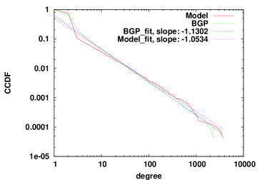
(a) Degree distribution

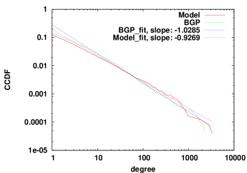
(b) Customer distribution

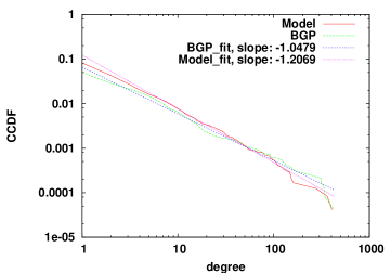
(c) Peer distribution

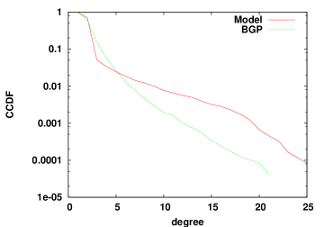
(d) Provider distribution

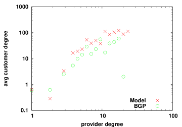
(e) Provider vs. cust. degree

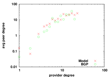
(f) Provider vs. peer degree

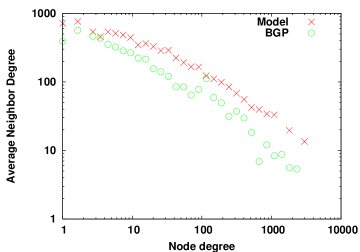
(g) Node total degree vs. the average degree of its customers and providers

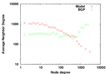
(h) Node total degree vs. the average degree of its peers

Figure 4: Validation of the MPA model by simulation.

We have developed a model that describes the evolution of the AS-level topology and validated the analytical results using measured parameters. We now simulate the MPA model using all of the measured parameters.

The MPA model generates annotated graphs, with links connecting either customers to providers (c2p links) or peers to peers (p2p links). Therefore the total node degree is a sum of the degrees of three types—the numbers of customers, providers, and peers attached to a node. Dimitropoulos et al. Dimitropoulos et al. (2009) have shown that the $2K$-annotated distribution of the Internet essentially defines its structure. In other words, if one randomizes the Internet preserving its $2K$-annotated distribution, then the randomized topologies will be almost identical to the original Internet topology. The $2K$-annotated distribution is a generalization of the joint degree distribution for graphs with links annotated by their types. These types can be abstracted by colors, and the traditional scalar node degree becomes a vector of colors specifying how many links colored by what colors are attached to the node. In the Internet case, these colors are customer, provider, and peer. The $2K$-annotated distribution is then the joint distribution for the vectors of colored degrees of nodes connected by differently colored links.

Given the findings in Dimitropoulos et al. (2009), in order to show that our model reproduces the Internet structure, it suffices to compare the $2K$-annotated distributions in simulated networks and the Internet. Unfortunately, the $2K$-annotated distribution is too multi-dimensional and sparse. Therefore, we can work only with its projections. The reasonable and informative projections include Dimitropoulos et al. (2009): (i) the degree distribution (DD): the traditional distribution of total node degrees, i.e., the number of links of all types attached to a node; (ii) the annotated distributions (ADs): the distributions of the number of customers, providers, and peers that nodes have, i.e., the distribution of degrees of each type; (iii) the annotated degree distribution (ADD): the joint distribution of customers, providers, and peers of nodes, measuring the per-node correlations among these three degree types; and (iv) the joint degree distributions (JDDs): the JDDs measure the correlations of total node degrees “across the links” of different types.

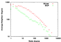
(a) Average neighbor degree

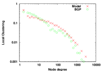
(b) Clustering

Figure 5: Average neighbor degree and clustering in simulations vs. real data.

Therefore, in our validation we compare all these metrics between the graphs that the MPA-model produces and the Internet topology annotated with AS relationships using Dimitropoulos et al. (2007) on Jan 1, 2007. The specific dataset used is http://as-rank.caida.org/data/2007/as-rel.20070101.a0.01000.txt, which is a part of CAIDA providing publicly available weekly snapshots of the annotated Internet. These snapshots are based on the Route Views BGP data rou . The values of the parameters we use in our simulations are $\rho=2.3$, $\nu=1$, $c=0.704$, and $m=1.86$, which we recall are the ratio of the numbers of non-ISPs to ISPs, ratio of ISP multihoming links to ISPs, ratio of peering links to ISPs, and the average number of providers to which non-ISPs multihome, respectively. We run the simulation with deterministic link arrivals based on their arrival rates. The total number of ISP and non-ISP nodes are $7,200$ and $16,800$. These are the numbers of nodes that we were able to classify in the dataset using Dimitropoulos et al. (2006). We do not model bankruptcy since as mentioned earlier, the rate at which it occurs is too small to get an accurate estimate of our bankruptcy ratio $\mu$.

Degree Distribution (DD): Figure 4(a) shows the DD of the graphs generated by the MPA model, and its comparison with the observed topology. As predicted in the Section III the MPA model produces a power law DD, and the exponent of the CCDF matches well the BGP data.

Annotated Distributions (AD): Figures 4(b)–4(d) show the ADs generated by the MPA model. We compare the customer, peer, and provider degree distributions of the simulated graph with that of the BGP tables. As predicted, the ADs of number of customers and peers are both power law graphs with the same exponent as the DD.

We plot the CCDF of the number of providers that ISPs multihome to (on linear $x$-axis and logarithmic $y$-axis) in Figure 4(d). They are approximately of form $1+X$, where $X$ is exponentially distributed. The curves show a discrepancy in slope. We believe that it arises due to the fact that almost all the distribution mass is concentrated at small degrees, as the mean is $2$, and the number of ISPs with high multihoming degree is small.

Annotated Degree Distribution (ADD): Each ISP has some numbers of providers, peers, and customers. The ADD is the joint distribution of these numbers across all observed ISPs. We illustrate these correlations in Figures 4(e) and 4(f). To construct these plots, we first bin the ISP nodes by the number of providers that they have (the $x$-axis), and then compute the average number of customers or peers that the ISPs in each bin have (the $y$-axis). We observe that the MPA model approximately matches the BGP data against these metrics as well.

Joint Degree Distributions (JDDs): While the ADD contains information about the correlations between the numbers of different types of nodes connected to an ISP, it does not reveal information about the degree correlations between the parameters of different ISPs connected to each other, i.e., whether higher degree ISPs are more likely to peer with each other, etc. This information is contained in the average neighbor connectivity, which is a summary statistic of the joint degree distributions in Figures 4(g) and 4(h). Specifically, let the probability that a node of degree $k$ has a c2p link to a node of degree $k^{\prime}$ be called $P_{c2p}(k^{\prime}|k)$. Then the average degree of the provider ISPs of ISPs that have degree $k$ is $\bar{k}_{c2p}(k)=\sum_{k}^{\prime}k^{\prime}P_{c2p}(k^{\prime}|k)$. In a full mesh graph with $n$ nodes and undirected links, since all nodes have degree $n-1$, the value of this coefficient is simply $n-1$. We show the normalized value $k_{c2p}(k)/(n-1)$ in Figure 4(g). The similarly normalized values of $\bar{k}_{p2p}(k)$ are shown in Figure 4(h). These functions exhibit similar behaviors for the MPA model and BGP data.

Coupled with observations in Dimitropoulos et al. (2009) that the real Internet topology is accurately captured by its $2K$-annotated distribution, the results in this section provide evidence that the MPA model reproduces closely the Internet AS-level topology across a wide range of metrics. As an example, we show in Figure 5 two standard topology metrics: the average neighbor degree and clustering as functions of the total node degree. We observe that even though two-class preferential attachment in Section II produces tree networks, its multiclass extensions in Section III, implemented in our simulations, closely reproduce clustering observed in the real Internet, which is a consequence of the $2K$-annotated randomness of the Internet, and the $2K$-annotated distribution match in Figure 4. Finally, the average total node degree in the real Internet and simulations is $4.1$ and $4.2$ respectively.

VI Conclusion

We constructed a realistic and analytically tractable model of the Internet AS topology evolution that we call the multiclass preferential attachment (MPA) model. The MPA model is based on preferential attachment, and we believe it uses the minimum number of measurable parameters altering standard preferential attachment to produce annotated topologies that are remarkably similar to the real AS Internet topology. Each model parameter reflects a realistic aspect of AS dynamics. We measure all parameters using publicly available AS topology data, substitute them in our derived analytic expressions for the model, and find that it produces topologies that match observed ones against a definitive set of network topology characteristics. These characteristics are projections of the second-order degree correlations, annotated with AS business relationships. Matching them ensures that synthetic AS topologies match the real one according to all other important metrics Mahadevan et al. (2006a); Dimitropoulos et al. (2009).

The model parameter that has the most noticeable effect on the properties of generated topologies reflects the ratio of ISP to non-ISP ASs. Contrary to common beliefs, the parameters taking care of AS peering, bankruptcies, multihoming, etc., are less important, as far the degree distribution is concerned, although they do affect other network properties, such as clustering. No other parameters or complicated mechanisms appear to be needed to explain the Internet topology annotated with AS business relationships. In other words, preferential attachment, with the MPA modifications, appears to explain the complexity of the AS-level Internet abstracted as an annotated graph. An interesting open question concerns the origins of preferential attachment in the Internet. Given that the vast majority of AS links connect customer ASs to their providers Dimitropoulos et al. (2007), this question reduces to finding how customers select their providers. The popularity of providers, their “brand names,” may be an important factor explaining the preferential attachment mechanism acting in the Internet.