Renormalization group approach to the P versus NP question

Abstract

This paper argues that the ideas underlying the renormalization group technique used to characterize phase transitions in condensed matter systems could be useful for distinguishing computational complexity classes. The paper presents a renormalization group transformation that maps an arbitrary Boolean function of $N$ Boolean variables to one of $N-1$ variables. When this transformation is applied repeatedly, the behavior of the resulting sequence of functions is different for a generic Boolean function than for Boolean functions that can be written as a polynomial of degree $\xi$ with $\xi\ll N$ as well as for functions that depend on composite variables such as the arithmetic sum of the inputs. Being able to demonstrate that functions are non-generic is of interest because it suggests an avenue for constructing an algorithm capable of demonstrating that a given Boolean function cannot be computed using resources that are bounded by a polynomial of $N$.

1 Introduction

Computational complexity characterizes how the computational resources to solve a problem depend on the size of the problem specification [1]. Two well-known complexity classes [2] are P, problems that can be solved with resources that scale polynomially with the problem size, and NP, the class of problems for which a solution can be verified with polynomial resources. Whether or not P is equal to NP [3, 4] is a great outstanding question in computational complexity theory and in mathematics generally [5, 6, 7, 8, 9].

In this paper it is argued that a method known in statistical physics as the renormalization group (RG) [11, 12, 13, 10] may yield useful insight into the P versus NP question. This technique, originally formulated to provide insight into the nature of phase transitions in statistical mechanical systems [11, 12], involves taking a problem with $N$ variables and then rewriting it as a problem involving fewer variables. Here, we will define a procedure by which a given Boolean function of $N$ Boolean variables is used to generate a Boolean function of $N-1$ variables, and investigate the properties of the resulting sequence of functions as this procedure is iterated [14]. The transformation used here is very simple — the new function is one if the original function changes its output value when a given input variable’s value is changed, and is zero if it does not. It is shown that when this transformation is applied repeatedly, the behavior of the resulting sequence of functions can be used to distinguish generic Boolean functions from functions that are known to be computable using polynomially bounded resources.

Any Boolean function $f(x_{1},\ldots,x_{N})$ of the $N$ Boolean variables $x_{1},\ldots,x_{N}$ can be written as a polynomial in the $x_{j}$ using modulo-two addition. This follows because the variables and function all can be only $0$ or $1$, so $f(x_{1},\ldots,x_{N})$ can be written as

$$f(x_{1},\ldots,x_{N}) = A_{00\ldots 00}(1\oplus x_{1})(1\oplus x_{2})\ldots(1\oplus x_{N-1})(1\oplus x_{N})$$ (1)

$$\oplus A_{00\ldots 01}(1\oplus x_{1})(1\oplus x_{2})\ldots(1\oplus x_{N-1})(x_{N})$$

$$\ldots$$

$$\oplus A_{11\ldots 10}(x_{1})(x_{2})\ldots(x_{N-1})(1\oplus x_{N})$$

$$\oplus A_{11\ldots 11}(x_{1})(x_{2})\ldots(x_{N-1})(x_{N})~{},$$

where $A_{x_{1},\ldots,x_{N}}=f(x_{1},\ldots,x_{N})$. As Shannon pointed out [15], the number of different possible functions is $2^{2^{N}}$ (this follows because each of the $2^{N}$ coefficients $A_{\alpha_{1},\ldots,\alpha_{N}}$ can be either one or zero). This is much larger than the number of functions that can be computed using resources that scale no faster than as a polynomial of $N$, which scales asymptotically as $(CN)^{t}$, where $C$ is a constant and $t$ is a polynomial in $N$ [16, 17]. This counting argument demonstrates that almost all functions cannot be evaluated using polynomially bounded resources and hence are not in P. However, it does not provide a means for determining whether or not a given function can be computed with polynomial resources.

It is shown here that different classes of functions have different behavior upon repeated application of a renormalization group transformation. In analogy with well-known results in statistical mechanics [10], we interpret functions exhibiting different behaviors after many renormalizations as being in different phases. Generic Boolean functions exhibit simple “fixed point” behavior upon renormalization, and hence we claim that they comprise a phase. A function that can be written either as a low-order polynomial or as a function of a composite variable such as the arithmetic sum of the values of the inputs yields non-generic behavior upon renormalization, and so is in a non-generic phase.

We then discuss what would be needed to be able to use the renormalization group approach to demonstrate that a given Boolean function of $N$ variables cannot be evaluated with resources that are bounded above by a polynomial in $N$. This issue is relevant to the P versus NP question because if we can identify a function in NP that we can show is not in P, then we will have shown that P and NP are not equal. Some functions that are in P depend on the arithmetic sum of the inputs, including MAJORITY, which is one if more than half the inputs are nonzero and zero otherwise [18], and DIVISIBILITY MOD $p$, which is one if the sum of the inputs is divisible by an odd prime $p$ [20, 19], and the renormalization group approach identifies these functions as non-generic. The renormalization group approach identifies low-order polynomials as non-generic, and some but not all low-order polynomials are in P. Because there are functions in P that are the sum of a low-order polynomial plus a small random component that is nonzero on a small fraction of the inputs, and because such functions will “flow” to the generic fixed point upon renormalization, P is not a phase in the statistical mechanical sense. Therefore, there are functions known to be in P that can be identified as non-generic only because they are close to a phase boundary in the sense that they differ from a low-order polynomial on a small fraction of the inputs. Thus, the renormalization group approach provides a means for understanding why the P versus NP question is so difficult — showing that a function is not in P using the renormalization group approach requires determining not only that it is not in a non-generic phase but also that it is not near a phase boundary, a task that appears to require resources that grow faster than exponentially with $N$. This superexponential scaling means that the procedure proposed here cannot be used to break pseudorandom number generators, a difficulty that would arise if the procedure could be implemented with resources that scale no faster than exponentially with $N$ [21]. However, at this point we cannot prove that a given function is not in P—our procedure distinguishes every function in P of which we are aware from a generic Boolean function, but we have not demonstrated that the procedure works for all functions that are in P.

The paper is organized as follows. Sec. 2 presents the transformation that maps a Boolean function of $N$ variables into a Boolean function of $N-1$ variables. Repeatedly applying this transformation yields a sequence of functions, and in Sec. 2 it is shown that (1) if one starts with a generic random Boolean function, then the resulting sequence of functions has the property that all functions in it are nonzero for just about half the input configurations, (2) applying the RG transformation $\xi$ times to a function that is a polynomial of order less than $\xi$ yields zero, and (3) applying the RG transformation to functions that depend on a composite variable such as the sum of the values of all the inputs also yields a sequence of functions that differs from from the result for a generic Boolean function. In Sec. (3) it is shown that simply applying the RG transformation many times does not identify functions that can be written as the sum of a low-order polynomial plus a contribution that is nonzero on a small fraction of the inputs. One can identify functions of this type by examining the set of functions whose outputs differ from the original one on a small fraction of the input configurations — one of the functions in the set will be a low-order polynomial. Sec. 4 discusses the results in the framework of phase transitions in condensed matter systems, which renormalization group transformations are typically used to study, and also discusses how the strategy discussed here avoids the difficulties of “natural proofs” described in Ref. [21]. Sec. 5 presents the conclusions. Appendix A presents the arguments demonstrating why it is plausible most functions that can be computed with polynomially bounded resources can be written as a low-order polynomial plus a term that is nonzero for a fraction of input configurations that is exponentially small in $N/\log(N)$, and discusses the non-generic nature of the functions in P that do not have that property. Appendix B shows that a typical Boolean function cannot be written as a low-order polynomial plus a term that is exponentially small in $N/\log(N)$.

2 Renormalization group transformation

The renormalization group (RG) procedure we define takes a given function of $N$ variables and generates a function of $N-1$ variables [10, 11, 12, 13, 14]. The variable that is eliminated is called the “decimated” variable. The procedure can be iterated, mapping a function of $N-1$ variables into one of $N-2$ variables, etc.

The transformation studied here specifies whether the original function’s value changes if a given input variable is changed. Specifically, given a function $f(x_{1},\ldots,x_{N})\equiv f(\vec{x})$, we define

$$g_{i_{1}}(x_{1},x_{1},\ldots,x_{i_{1}-1},x_{i_{1}+1},\ldots,x_{N})\equiv g_{i_{1}}(\vec{x}^{\prime})$$ (2)

$$~{}~{}=f(x_{1},x_{2},\ldots,x_{i_{1}-1},0,x_{i_{1}+1},\ldots,x_{N})\oplus f(x_{1},x_{2},\ldots,x_{i_{1}-1},1,x_{i_{1}+1},\ldots,x_{N})~{},$$

where $\oplus$ denotes addition modulo $2$ [22], and the vector $\vec{x}^{\prime}$ denotes the set of undecimated variables. The function $g_{i_{1}}(x_{1},x_{2},\ldots,x_{i_{1}-1},x_{i_{1}+1},\ldots,x_{N})$ is one if the output of the function $f$ changes when the value of the decimated variable $x_{i_{1}}$ is changed and zero if it does not. Once $g_{i_{1}}$ has been obtained, the procedure can be repeated and one can define $g_{i_{1},i_{2}}$ as

$$g_{i_{1},i_{2}}(x_{1},x_{1},\ldots,x_{i_{1}-1},x_{i_{1}+1},\ldots,x_{i_{2}-1},x_{i_{2}+1},x_{N})\equiv g_{i_{1},i_{2}}(\vec{x}^{\prime})$$ (3)

$$=~{}~{}g_{i_{1}}(x_{1},x_{2},\ldots,x_{i_{2}-1},0,x_{i_{2}+1},\ldots,x_{N})$$

$$~{}~{}\oplus g_{i_{1}}(x_{1},x_{2},\ldots,x_{i_{2}-1},1,x_{i_{2}+1},\ldots,x_{N})$$

$$=~{}~{}~{}f(x_{1},x_{2},\ldots,x_{i_{1}-1},0,x_{i_{1}+1},\ldots,x_{i_{2}-1},0,x_{i_{2}+1},\ldots,x_{N})$$

$$~{}~{}~{}\oplus f(x_{1},x_{2},\ldots,x_{i_{1}-1},0,x_{i_{1}+1},\ldots,x_{i_{2}-1},1,x_{i_{2}+1},\ldots,x_{N})$$

$$~{}~{}~{}\oplus f(x_{1},x_{2},\ldots,x_{i_{1}-1},1,x_{i_{1}+1},\ldots,x_{i_{2}-1},0,x_{i_{2}+1},\ldots,x_{N})$$

$$~{}~{}~{}\oplus f(x_{1},x_{2},\ldots,x_{i_{1}-1},1,x_{i_{1}+1},\ldots,x_{i_{2}-1},1,x_{i_{2}+1},\ldots,x_{N})~{},$$

where the sums all denote addition modulo two. The function $g_{x_{i_{1}},\ldots,x_{i_{m}}}(\vec{x}^{\prime})$ obtained by decimating the $m$ variables $x_{i_{1}},\ldots,x_{i_{m}}$ does not depend on the order in which the variables are decimated.

First we examine functions for which each of the coefficients $A_{\alpha_{1},\alpha_{2},\ldots,\alpha_{N}}^{(0)}$ in Eq. (1) is an independent random variable chosen to be one with probability $p_{0}$ and zero with probability $q_{0}=1-p_{0}$, where $0<p_{0}<1$. We consider the sequence of functions obtained by successive application of the renormalization group transformation to such a generic random function. The coefficients $A^{(i_{1})}_{x_{1},\ldots,x_{i_{1}-1},x_{i_{1}+1},\ldots,x_{N}}$ that characterize the function $g_{i_{1}}(\vec{x}^{\prime})$ obtained by decimating the variable $i_{1}$ via Eq. (2) are

$$A^{(i_{1})}_{x_{1},\ldots,x_{i_{1}-1},x_{i_{1}+1},\ldots,x_{N}}=A_{x_{1},\ldots,x_{i_{1}-1},0,x_{i_{1}+1},\ldots,x_{N}}\oplus A_{x_{1},\ldots,x_{i_{1}-1},1,x_{i_{1}+1},\ldots,x_{N}}~{}.$$ (4)

The original $A^{(0)}$’s are uncorrelated random variables, so it follows that the $A^{({i_{1}})}$’s are independent random variables that are one with probability $p_{1}=2p_{0}q_{0}$ and zero with probability $1-p_{1}$. After $\ell$ iterations (after which $\ell$ variables have been eliminated), the coefficients are still uncorrelated random variables, and they are now one with probability $p_{\ell}$ and zero with probability $1-p_{\ell}$, where the $p_{\ell}$ satisfy the recursion relation

$$p_{\ell+1}=2p_{\ell}(1-p_{\ell})~{}.$$ (5)

The solution to Eq. (5) is

$$p_{\ell}=\frac{1}{2}\left(1-(1-2p_{0})^{2^{\ell}}\right).$$ (6)

For any $p_{0}$ satisfying $0<p_{0}<1$, the values of the $p_{\ell}$ “flow” as $\ell$ increases and eventually approach the “fixed-point value” of $1/2$ [10]. This behavior is exactly analogous to that displayed by the partition functions describing thermodynamic phases in statistical mechanical systems, and so we interpret this behavior as evidence that there is a phase of generic Boolean functions.

In Sec. (3) we will be considering values of $p_{0}$ that are very small but nonzero, for which case $p_{\ell}$ grows exponentially with $\ell$:

$$p_{\ell}=2^{\ell}p_{0}\qquad({\rm when~{}}p_{\ell}\ll 1)~{}.$$ (7)

After many renormalizations such functions will “flow” to the generic fixed point, so they are in the generic phase. If one chooses $p_{0}=P(N)2^{-N}$, where $P(N)$ is a polynomial in $N$, the function can be specified with polynomially bounded resources by enumerating all input configurations for which the function is nonzero.

Note that when the RG transformation is applied to a generic Boolean function, all the functions that are generated yield an output that is zero on a fraction of the inputs that differs from $1/2$ by an amount that is exponentially small in $N$. This follows because almost all Boolean functions have an initial value of $p_{0}$ that differs from $1/2$ by an amount that is the square root of the number of values chosen, or $(2^{N})^{1/2}=2^{N/2}$. Since all the $p_{\ell}$ deviate from $1/2$ by an amount that is exponentially small in $N$, and since the number of independent input configurations remains exponentially large in $N$ until the number of decimated variables is of order $N$, for every function obtained via the renormalization transformation, the fraction of input configurations yielding zero deviates from $1/2$ by an amount that is exponentially small in $N$.

We next demonstrate that Boolean functions that can be written as polynomials of degree of $\xi$ or less when $\xi<N$ have the property that they yield zero after $\xi+1$ renormalizations, for any choice of the decimated variables.

First we examine a simple example. The parity function $\mathcal{P}(x_{1},\ldots,x_{N})$, which is $1$ if an odd number of input variables are 1 and $0$ if an even number of the input variables are 1 [23, 24, 25, 9], can be written as

$$\mathcal{P}(x_{1},\ldots,x_{N})=x_{1}\oplus x_{2}\oplus\ldots\oplus x_{N}~{}.$$ (8)

There are many less efficient ways to write the parity function, but the result of the renormalization procedure does not depend on how one has chosen to write the function, since it can be computed knowing only the values of the function for all different input configurations. For the parity function, one finds, for any choice of decimated variables $x_{j_{1}}$ and $x_{j_{2}}$, the functions resulting from one and two renormalizations, $g^{P}_{j_{1}}(\vec{x}^{\prime})$ and $g^{P}_{i_{j_{1},j_{2}}}(\vec{x}^{\prime})$, are:

$$g^{P}_{j_{1}}(\vec{x}^{\prime})=x_{j_{1}}\oplus(1-x_{j_{1}})=1~{};$$

$$g^{P}_{i_{j_{1},j_{2}}}(\vec{x}^{\prime})=0~{}.$$

Thus, applying the renormalization transformation to the parity function yields zero after two iterations, in contrast to the behavior of a generic Boolean function.

More generally, for any term of the form $T=y_{i_{1}}y_{i_{2}}\ldots y_{i_{m}}$, with $y_{i}=x_{i}$ or $1-x_{i}$, the quantity $T(x_{i}=1)\oplus T(x_{i}=0)$ is either zero (if $y_{i}$ does not occur in $T$) or else is the product of $m-1$ instead of $m$ of the $y$’s; for example

$$T(y_{i_{1}}=1)\oplus T(y_{i_{1}}=0)=y_{i_{2}}\ldots y_{i_{m}}~{}.$$ (9)

Because the effect of the RG procedure on the sum of terms is equal to the sum of the results of the transformation applied to the individual terms, any function that is the mod-2 sum of terms that are all products of fewer than $m$ $y$’s will yield zero after $m$ renormalizations, for any choice of the decimated variables. It follows immediately that a function that is a polynomial of degree $\xi$ or less has the property that applying the RG transformation to it $\xi+1$ times yields zero for any choice of the decimated variables.

This result demonstrates that the RG transformation distinguishes generic Boolean functions from functions that can be written as polynomials of degree $\xi$ or less, when $\xi<N$. The qualitatively different behavior upon renormalization of polynomials of degree $\xi$ from generic Boolean functions can be interpreted as evidence that these two classes of functions are in different phases.

We now demonstrate that the RG method also identifies as non-generic functions that depend on a composite quantity such as the arithmetic sum of the variables. Functions in P with this property include MAJORITY (which is one if more than half the inputs are set to one, and zero otherwise) [18] and DIVISIBILITY MOD p (which is one if the number of inputs that are set to one is divisible by an odd prime p and zero otherwise) [20, 19]. The renormalization group approach distinguishes such functions from generic Boolean functions because the output of all the functions in the sequence is constrained to be identical for very large sets of input configurations. We first show that MAJORITY and DIVISIBILITY MOD p are both distinguished from a generic Boolean function by the renormalization group procedure, and then we argue that the RG procedure distinguishes any function of the arithmetic sum of the inputs from a generic Boolean function. We expect that the argument will be generalizable to apply to a broad class of functions that depend on other composite quantities that are specific combinations of the input variables.

First we consider the behavior when the RG transformation is applied to DIVISIBILITY MOD 3. Since this function is nonzero when the arithmetic sum $\sum_{j=1}^{N}x_{j}$ is divisible by $3$, changing an input $x_{i}$ changes the output value when the sum of the other input variables is either zero or two. Thus, the renormalized function $g_{i}(\vec{x}^{\prime})$ is nonzero for any $i$ on a fraction of the input configurations that is very close to $2/3$. Every succeeding renormalization also yields a function that is nonzero when the sum of the remaining variables is either zero or two. This behavior differs from that of a generic Boolean function, in which the renormalized functions are nonzero for a fraction of inputs that is very close to $1/2$. More generally, when the RG is applied to DIVISIBILITY MOD p, with p an odd prime, the behavior of the sequence of functions is determined by the value of the mod p remainder of the undecimated variables. The functions in the sequence yield the output one when the remainder mod p takes on certain values, and typically, after a small number of iterations, these values cycle with a finite period. Therefore, the fraction of input configurations that lead to a nonzero input essentially cycles also (the cycling is not exact only because the fraction of input configurations with a given value of the remainder mod p changes very slightly with $N$), and, since p is odd, none of the fractions in the cycle is close to $1/2$.

The behavior obtained when the RG procedure is applied to the MAJORITY function is also significantly different from that of a generic Boolean function. The first renormalization step yields a function that is nonzero when the sum of the undecimated variables is $N/2-1$, and the second step yields a function that is nonzero when the sum of the undecimated variables is either $N/2-2$ or $N/2-1$. The functions obtained after $j$ decimations are nonzero on a fraction of inputs that is bounded above by $Cj/\sqrt{N}$, where $C$ is a constant of order unity, so long as $j\ll\sqrt{N}$. The original function is thus identified as non-generic because so long as the number of renormalizations applied is much smaller than $\sqrt{N}$ the renormalized functions are all nonzero on a fraction of input configurations that is much less than $1/2$.

Next we argue that the renormalization group approach distinguishes any function of the arithmetic sum of the inputs from a generic Boolean function. The physical intuition underlying the argument is that all the functions in the sequence depend only on the arithmetic sum of the undecimated variables, and when the number of undecimated variables is $\mathcal{N}$, the number of configurations of the undecimated variables whose arithmetic sum is constrained to be $\mathcal{S}$, is $\mathcal{N}!/\mathcal{S}!(\mathcal{N}-\mathcal{S})!$. One can use Stirling’s series [28] to show explicitly that when $N$ is large, then the number of configurations with a given value of $\mathcal{S}$ is a polynomial in $1/N$ times $2^{N}$ for a number of values of $\mathcal{S}$ that grows as the square root of $N$. Therefore, the differences in the fraction of configurations yielding different values of $N$ decay polynomially with $N$, and the fraction of input configurations yielding one should either be exactly 1/2 or else must deviate from 1/2 by an amount that decreases only polynomially with $N$.

3 Renormalization procedure for characterizing functions that can be constructed using polynomially bounded resources.

This section addresses the relationship between non-generic phases of Boolean functions and the computational complexity class P of functions that can be computed with polynomially bounded resources.

There are functions that are in P that are neither polynomials of degree $\xi$ with $\xi<N$ nor functions of composite variables. For example, because the sum of two functions that are in P is in P, a sum of any function that is in P with a small “generic” piece specified by Eq. (1) with the coefficients chosen independently and randomly to be one with probability $p_{0}=\mathcal{P}(N)2^{-N}$, where $\mathcal{P}(N)$ is a polynomial in $N$, is in P. Eq. (7) shows that $\ell$ renormalizations cause the value of $p_{\ell}$ to grow exponentially with $\ell$, $p_{\ell}=2^{\ell}p_{0}$; in renormalization group parlance [10] the remainder is a “relevant” perturbation. Since the generic piece renormalizes towards the generic fixed point at which exponentially close to half the inputs yield a nonzero output, whether or not the function resulting from many renormalizations can be identified as non-generic depends on whether the first piece yields a nonzero result after many renormalizations. A function of a composite variable yields a result different both from zero and from that of generic functions, and when a small generic piece is added to such a function, renormalization still yields a non-generic result. However, because after $\xi+1$ renormalizations of a polynomial of order $\xi$ one obtains zero, renormalizing functions that are the sum of a low-order polynomial and a small generic piece yields zero plus the generic result, and so cannot be identified as non-generic by straightforward application of the renormalization transformation.

The number of polynomials of $N$ variables with degree $\xi$ is $2^{\sum_{k=1}^{\xi}N!/(\xi!(N-\xi)!)}$ [26], which when $\xi\ll N$ can be approximated as $2^{e(N/\xi)^{\xi}}$. Therefore, when $\xi$ scales as a fractional power of $N$, there are many more polynomials of degree $\xi$ than there are functions in P. On the other hand, the product of all $N$ variables $x_{1}\ldots x_{N}$ is in P, so there are functions in P that cannot be written as polynomials of degree $\xi$ for any $\xi<N$. Therefore, using our definition of a phase based on the behavior yielded by repeated renormalization, P is not a phase. There are non-generic functions that are not in P and there are functions in P that are in the generic phase. However, note that a product of $M$ variables is nonzero for only a fraction $2^{-M}$ of the input configurations. For example, the term $x_{1}x_{2}\ldots x_{R}$ is nonzero only for input configurations that have $x_{1}=x_{2}=\ldots=x_{R}=1$. The sum of a polynomially large number $M$ of terms of this type is nonzero only on a fraction of inputs that is bounded above by $M/2^{R}$. In Appendix A it is argued that the functions in P that are in the generic phase have the property that for any $\xi<N$, any Boolean function of $N$ variables $f(x_{1},\ldots,x_{N})$ that is in P can be written as the sum:

$$f(x_{1},\ldots,x_{N})=\mathcal{P}_{\xi}(x_{1},\ldots,x_{N})\oplus\mathcal{R}_{\xi}(x_{1},\ldots,x_{N})~{},$$ (10)

where $\mathcal{P}_{\xi}(x_{1},\ldots,x_{N})$ is a polynomial of degree no more than $\xi$ and the remainder term $\mathcal{R}_{\xi}(x_{1},\ldots,x_{N})$ is nonzero on a fraction of input configurations that is bounded above by $\mathcal{C}2^{-\alpha\xi/\log_{2}(N)}$, with $\mathcal{C}$ and $\alpha$ positive constants.

As discussed above, using the RG transformation to identify functions that satisfy Eq. (10) is not entirely straightforward — the obvious strategy, seeing if the functions obtained after renormalizing $\xi+1$ times have a small remainder term, fails because renormalization yields exponential growth in the fraction of input configurations for which the remainder term is nonzero. This difficulty can be circumvented by examining all functions that differ from the function in question on a fraction of input configurations no greater than $\mathcal{C}2^{-\alpha\xi/\log_{2}(N)}$. If the original function obeys Eq. (10), then one of the “perturbed” functions will have a remainder term that is zero, and applying the renormalization transformation to it $\xi+1$ times yields zero for all choices of the decimated variables.

There are functions known to be in P that can written as the sum of a function of a composite variable plus a function that is nonzero on a small fraction of inputs. Nongeneric behavior is obtained upon renormalization for all such functions except for those for which all functions in the renormalization sequence yield one for exactly half the input configurations. The procedure for identifying such functions is exactly analogous as for identifying functions that can be approximated as low-order polynomials — examine the properties under renormalization of all the functions that are yield the same output as the one in question except for a small fraction of the inputs.

Finally, we note that in Appendix B it is demonstrated that almost all generic random functions do not satisfy Eq. (10) when $\xi$ scales as a fractional power of $N$.

4 Discussion

This paper presents a renormalization group approach that distinguishes generic Boolean functions of $N$ variables from functions that can be written as a polynomial of degree $\xi$, with $\xi\ll N$, and also from functions that depend only on composite quantities such as the arithmetic sum of all the input variables. The method provides a consistent framework for identifying many different functions as non-generic.

The renormalization group approach also provides a natural framework for understanding why the P versus NP question is so difficult. Functions computable with polynomial resources do not comprise a phase — there are functions that are in a non-generic phase that are not in P, and there are functions in P for which the renormalization group yields a “flow” that is towards the generic fixed point and hence are in the “generic” phase. The possibility of using the RG approach to demonstrate that a given Boolean function is not in P arises because it is possible that all functions in P that are in the generic phase are all close to a phase boundary of a non-generic phase. Whether the renormalization group approach can provide a means for determining whether or P is distinct from NP depends on whether it is possible to demonstrate that all efficiently computable functions are in or near a non-generic phase.

The procedure used here of using the behavior yielded by a renormalization group transformation to identify different phases of Boolean functions is entirely analogous to a procedure presented by Wilson [13] to identify different thermodynamic phases of the Ising model, used to describe magnetism in solids. Wilson showed that individual configurations of Ising models could be identified as being in either a ferromagnetic phase or paramagnetic phase by repeatedly eliminating spins and examining the resulting configurations — if after many renormalizations all the spins are aligned, then the system is in the ferromagnetic phase, while if after many renormalizations the spin orientations are random, then the system is in the paramagnetic phase. Viewing the analogy between the results for magnets and the qualitatively different behavior of the renormalization group “flows” for polynomials of degree $\xi$, for functions of composite variables, and for generic Boolean functions as an indication that low-degree polynomials and functions of composite variables are both non-generic “phases,” we propose the schematic phase diagram for Boolean functions, shown in Fig. 1.

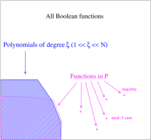
Figure 1: Schematic phase diagram for Boolean functions. Within the set of all Boolean functions of $N$ Boolean variables there is a generic phase, a phase consisting of functions that can be written as polynomials of order no greater than $\xi$ with $\xi\ll N$, and there are phases corresponding to functions of composite variables such as the arithmetic sum of all the inputs. Some polynomials of degree $\xi$ are not in P, and some functions that can be computed with polynomial resources cannot be written either as polynomials of degree $\xi$ for any $\xi<N$ or as functions of a composite variable. Therefore, P does not denote a phase. However, we conjecture that that all functions in P are either in a non-generic phase or else very close to the low-order-polynomial phase boundary.

If it can be shown that all functions in P are either in a non-generic phase or else very close to a phase boundary, then the procedure described here leads to a specific algorithmic approach to the P versus NP question — if a given function that is obtained as the answer to a problem in NP fails to be close enough to a non-generic phase, then one has shown that P is not equal to NP. (Ref. [29] advocates a family of candidate functions for testing using the strategy proposed in this paper, but the strategy can be implemented for any candidate function.) Appendix B shows that almost all Boolean functions are not close to non-generic phase boundaries. Appendix A argues that the construction of a function in P that does not satisfy Eq. (10) requires delicate balancing that may signal the existence of a composite variable, but the argument is only speculative. Progress on this issue is the key to using the RG approach to be able to address the P versus NP question.

Because the procedure discussed in Sec. 3 requires a number of operations that scales superexponentially with N, the procedure proposed here is not a “natural proof” as discussed in Ref. [21] and therefore does not yield a method for breaking pseudorandom number generators. However, direct numerical implementation of the procedure is not likely to be computationally feasible.

5 Conclusions

This paper presents a renormalization group approach that can be used to distinguish a generic Boolean function from (1) a Boolean function of $N$ variables that can be written as a polynomial of degree $\xi$ with $\xi<N$, and (2) a function that depends only on a composite variable (such as the arithmetic sum of the inputs). An algorithm for determining whether a function differs from a polynomial of degree $\xi$ on a fraction of inputs that is exponentially small in $\xi/\log(N)$ is presented. The possible relevance of these results to the question of whether P and NP are distinct is discussed.

6 Acknowledgments

The author is grateful to Prof. Daniel Spielman for pointing out a serious error in the original version of the manuscript, and for support from NSF grants CCF 0523680 and DMR 0209630.

Appendix A    Characterization of the functions that can be constructed with a polynomially large number of operations.

In this appendix we examine the properties of functions that can be computed with polynomially bounded resources. First we discuss why it is plausible that almost all functions in P can written in the form Eq. (10), which is the sum of two terms, the first a polynomial of degree $\xi$, and the second a correction term that is nonzero on a fraction of input configurations that is exponentially small in $\xi/\log(N)$. We then examine known functions in P that cannot be written in this form, arguing that they have special properties that may give rise to the emergence of a composite variable on which the function depends, which would lead to non-generic behavior upon renormalization.

To see why it is hard to construct functions in P that do not satisfy Eq. (10), we consider the process by which functions can be constructed. First we show that a starting polynomial that is the sum of polynomially many terms whose factors are all either $x_{i}$ or $(1-x_{i})$ satisfies Eq. (10). Then we show that the sum of two functions that each obey Eq. (10) also satisfies Eq. (10), and also that the coefficient multiplying the correction term grows sufficiently slowly that the bound remains true even after a number of additions that grows polynomially with $N$. We then consider products of such functions. The behavior is more complicated, but we argue that a similar decomposition works in most circumstances because when many terms are multiplied together, the result is nonzero only on a small fraction of inputs. Finally, we examine some functions in P which do not satisfy Eq. (10) and note that they involve a delicate balance that enables the sum of a finite number of products to be nonzero on the same fraction of inputs as the individual terms. It is plausible that this nongeneric property is associated with the nongeneric behavior of these functions upon renormalization.

First consider a polynomial $A(x_{1},\ldots,x_{N})$ that is the mod-2 sum of polynomially many terms that are all of the form $y_{i_{1}}\ldots y_{i_{m}}$, where $y_{i}$ is either $x_{i}$ or $1-x_{i}$:

$${A}(x_{1},\ldots,x_{N})=C_{0}+\sum_{\eta=1}^{N}\sum_{k_{\eta}=1}^{M_{\eta}}y_{i_{1}(\eta,k_{\eta})}\ldots y_{i_{\eta}(\eta,k_{\eta})}~{}.$$ (11)

Here, $C_{0}$ is a constant, $\eta$ denotes the number of factors of $y_{i}$ in a term, $k_{\eta}$ is the index labeling the different terms with $\eta$ factors, $i_{j}(\eta,k_{\eta})$ denotes the index of the $j^{th}$ factor in the term $k_{\eta}$, and each $M_{\eta}$, the number of terms with $\eta$ factors, is bounded above by a polynomial of $N$. We will obtain bounds on the number of configurations for which the output is nonzero by considering standard addition instead of modulo-two addition, which means that we will overcounting by including configurations for which an even number of terms in the polynomial expansion are nonzero. Each term with $\eta$ factors is nonzero only on a fraction $2^{-\eta}$ of the inputs. Therefore, if we define $\rho_{A}(\eta)$ to be the fraction of inputs of $A(x_{1},\ldots,x_{N})$ for which the sum of all the terms with $\eta$ factors is nonzero, we have

$$\rho_{A}(\eta)\leq C_{A}2^{-\alpha\eta}~{},$$ (12)

for constant $C_{A}$ and $\alpha=\frac{1}{2}-\epsilon$, with $\epsilon$ infinitesimal.

Now consider the addition of two functions $P(x_{1},\ldots,x_{N})$ and $Q(x_{1},\ldots,x_{N})$ that satisfy Eq. (10) for positive $\mathcal{C_{P}}$, $\mathcal{C_{Q}}$, and $\alpha$. Again we consider standard addition instead of modulo-two addition. Because the sum $S(x_{1},\ldots,x_{N})=P(x_{1},\ldots,x_{N})+Q(x_{1},\ldots,x_{N})$ has the property that all terms in the sum appears in at least one of the summands, we have

$$\rho_{S}(\eta)\leq\rho_{P}(\eta)+\rho_{Q}(\eta)~{};$$ (13)

the sum obeys Eq. (12) with the same value of $\alpha$ and with $C_{S}\leq C_{P}+C_{Q}$. Adding polynomially many terms can increase the prefactor only by an amount that grows no faster than polynomially in $N$.

We next consider the product of two functions that satisfy Eq. (12). We write

$$A(\vec{x}) = P_{A}^{\xi}(\vec{x})+R_{A}^{\xi}(\vec{x})$$

$$B(\vec{x}) = P_{B}^{\xi}(\vec{x})+R_{B}^{\xi}(\vec{x})~{},$$ (14)

where $P_{A}^{\xi}$ and $P_{B}^{\xi}$ are polynomials of order $\xi$ with $T_{A}$ and $T_{B}$ terms respectively, and $R_{A}^{\xi}(\vec{x})$ and $R_{B}^{\xi}(\vec{x})$ are both nonzero on a fraction of inputs that is less than $\mathcal{C}2^{-\alpha\xi}$ for positive constants $\mathcal{C}$ and $\alpha$.

We write the product of $A(\vec{x})$ and $B(\vec{x})$ as

$$D(\vec{x}) = A(\vec{x})B(\vec{x})$$ (15)

$$= (P_{A}^{\xi}(\vec{x})+R_{A}^{\xi}(\vec{x}))(P_{B}^{\xi}(\vec{x})+R_{B}^{\xi}(\vec{x}))$$

$$= P_{A}^{\xi}(\vec{x})P_{B}^{\xi}(\vec{x})+P_{A}^{\xi}(\vec{x})R_{B}^{\xi}(\vec{x})+R_{A}^{\xi}(\vec{x})P_{B}^{\xi}(\vec{x})+R_{A}^{\xi}(\vec{x})R_{B}^{\xi}(\vec{x})~{}.$$

Now $P_{A}^{\xi}(\vec{x})R_{B}^{\xi}(\vec{x})$ is nonzero on fewer inputs than $R_{B}^{\xi}(\vec{x})$ (this follows since a product is nonzero only if each of its factors is nonzero), and, similarly, $R_{A}^{\xi}(\vec{x})P_{B}^{\xi}(\vec{x})$ is nonzero on fewer inputs than either $R_{A}^{\xi}(\vec{x})$ or $R_{A}^{\xi}(\vec{x})$, so the sum of the last three terms must be less than $3\mathcal{C}2^{-\alpha\xi}$. Therefore, these contributions to the remainder term in the product remain exponentially small, with a coefficient that remains bounded by a polynomial in $N$ after polynomially many multiplications. Therefore, it only remains to consider the properties of the product $P_{A}^{\xi}(\vec{x})P_{B}^{\xi}(\vec{x})$, which we write

$$P_{A}^{\xi}(\vec{x})P_{B}^{\xi}(\vec{x})=P_{D}^{\xi}(\vec{x})+R_{D}^{\xi}(\vec{x})~{},$$ (16)

where $P_{D}^{\xi}(\vec{x})$ is a polynomial of degree $\xi$ and $R_{D}^{\xi}(\vec{x})$ is a remainder term that we need to bound.

To bound the magnitude of the remainder, let us multiply out the polynomials in Eq. (16) so that they are all sums of terms that are products of the form $y_{i_{1}}\ldots y_{i_{j}}$, terms that we will denote as “primitive.” Let $T_{A}$ be the number of primitive terms in $P_{A}^{\xi}(\vec{x})$, and $T_{B}$ be the number of primitive terms in $P_{B}^{\xi}(\vec{x})$. Note that every primitive term in the product with more than $\xi$ factors is nonzero on a fraction $2^{-\xi}$ or less of the input configurations.

Since the total number of primitive terms in $R_{D}^{\xi}(\vec{x})$ is bounded above by $T_{A}T_{B}$, the fraction of inputs on which the sum of the terms with at least $\xi$ factors is nonzero is bounded above by $T_{A}T_{B}2^{-\xi}$. So long as $T_{A}$ and $T_{B}$ are both less than exponentially large in $\xi$, then this remainder term is exponentially small in $\xi$. The multiplication process must start with values of $T_{A}$ and $T_{B}$ that are both bounded by a polynomial of $N$, but because multiplications can be composed, we need to examine the behavior of $T_{D}$, the number of primitive terms in $P_{D}^{\xi}(\vec{x})$.

A simple upper bound for $T_{D}$ is obtained by ignoring all possible simplifications that could reduce the total number of terms in the product:

$$T_{D}\leq T_{A}T_{B}~{}.$$ (17)

This equation describes geometric growth. If $\mathcal{M}$ polynomials are multiplied together, all of which have fewer than $CN^{Y}$ terms for fixed $C$ and $Y$, then the total number of terms in the product, $T_{\mathcal{M}}$, satisfies the bound

$$T_{\mathcal{M}}\leq(CN^{Y})^{\mathcal{M}}~{}.$$ (18)

This bound on the number of terms in the product is much smaller than $2^{\xi}$ so long as $\mathcal{M}$ satisfies

$$\mathcal{M}\ll\xi/(Y\log_{2}N+\log_{2}C)~{}.$$ (19)

A useful bound on multiplicative terms that are products of more than $\xi/(Y\log_{2}N)$ factors can be obtained by exploiting the fact that the product of two functions is nonzero for a given input only if each of the factors is. Specifically, consider the product $AB$, and say that $A$ is nonzero on a set of $M_{A}$ inputs. If $B$ is nonzero on less than a fraction $\sigma$ of the inputs in this set for some $1/2<\sigma<1$, then the product $AB$ is nonzero on fewer than $\sigma M_{A}$ inputs, and if not, then the product $A(1-B)$ is nonzero on fewer than $(1-\sigma)M_{A}$ inputs, and one can write $AB=A+A(1-B)$. [30]

The result of $\mathcal{M}$ multiplications is then nonzero only on a fraction of inputs bounded above by $2^{-\mathcal{M}\log_{2}\sigma}$. Therefore, a product of more than $\xi/Y\log_{2}(N)$ factors is nonzero on no more than a fraction $2^{-\tilde{C}\xi/\log_{2}(N)}$ of the inputs, where $\tilde{C}$ is a positive constant, and the entire product can be moved into the remainder term.

The arguments above indicate that the remainder term tends to be small for products because the number of terms in the polynomial that are of order $\xi$ or less can be bounded for products of small numbers of terms, and products of many terms are nonzero on a small enough fraction of the input configurations that they can be considered to be part of the remainder term. However, there are functions in P that do not obey Eq. (10). Two examples of functions that are in P that have been proven to violate Eq. (10) are MAJORITY (which is one when more than half input variables have been set to one and zero otherwise) [18] and DIVISIBILITY MOD p, which is one if the sum of the input variables is divisible by an odd prime p [20, 19]. Both these functions depend only on the arithmetic (not mod-2) sum of all the variables, $x_{1}+x_{2}+\ldots x_{N}$. Calculating the sum of $N$ variables can be done with polynomially bounded resources because one need only keep track of a running sum, which is the same for many different values of the individual $x_{j}$. For instance, when $k=N$, there are $N!/((N/2)!)^{2}\approx 2^{N}/\sqrt{2\pi N}$ different ways to choose the $x_{1}\ldots x_{k}$ so that their sum is $N/2$.

It is instructive to consider an algorithm for computing DIVISIBILITY MOD $3$ to see how the function avoids being a low order polynomial. Some pseudocode for a simple algorithm for this problem is:

$${\rm divisibility~{}mod~{}3:}$$

$$~{}~{}~{}~{}~{}{\rm start:remainder0[0]=1,remainder1[0]=remainder2[0]=0}$$

$$~{}~{}~{}~{}~{}{\rm for~{}each~{}i>0}$$

$$~{}~{}~{}~{}~{}{\rm remainder0[i+1]=remainder0[i]*(1-x_{i+1})\oplus remainder2[i]*x_{i+1}}$$

$$~{}~{}~{}~{}~{}{\rm remainder1[i+1]=remainder1[i]*(1-x_{i+1})\oplus remainder0[i]*x_{i+1}}$$

$$~{}~{}~{}~{}~{}{\rm remainder2[i+1]=remainder2[i]*(1-x_{i+1})\oplus remainder1[i]*x_{i+1}}$$

$$~{}~{}~{}~{}~{}{\rm answer=remainder0[N]}$$

The quantity remainder0[i]+remainder1[i]+remainder2[i] is unity for every i, and the fraction of inputs for which each remainder variable is nonzero is very close to $1/3$ and does not decay exponentially with i. The fractions do not decay or grow because the equation for each remainder for a given $i$ is the sum of two products. The product ${\rm remainder0[i](1-x_{i+1})}$ is nonzero on half the inputs on which remainder0[i] is nonzero, and similarly for the other term ${\rm remainder2[i]*x_{i+1}}$. Because ${\rm remainder0[i+1]}$ is the sum of two terms, each of which is nonzero on almost exactly half the outputs for which ${\rm remainder0[i]}$ is nonzero, ${\rm remainder0[j]}$ remains of order of but less than unity for all j. It is plausible that this exquisite cancellation leads to the existence of a composite variable on which the function depends, or, more generally, to non-generic behavior upon renormalization. Because obtaining a function that cannot be written as a low-order polynomial plus a term that is nonzero except for a small fraction of input configurations requires a series of delicate cancellations, it is also extremely plausible that the fraction of functions that are in P and do not satisfy Eq. (10) is extremely small.

As discussed in the main text, the renormalization group distinguishes functions that depend on the sum of the values of the input variables from generic Boolean functions because the renormalization transformation preserves the property that a given value for the composite variable occurs for an exponentially large numbers of input configurations. Moreover, at least when the composite variable is the arithmetic sum of the inputs, the fractions of input configurations for which the sum of the variables takes on different values differ by an amount that decays only polynomially with $N$. Therefore, such functions can yield one either on exactly half the inputs or else on a fraction of the inputs that differs from $1/2$ by an amount that is at least as large of $N^{-x}$ for some positive $x$.

To summarize, in this appendix we discuss the restrictions on Boolean functions of $N$ variables that can be computed with resources that are bounded above by a polynomial in $N$. Many functions in P have the property that they can be written, for any fixed $\xi$, as the sum of a polynomial of degree $\xi$ and a term that is bounded above by $\mathcal{C}2^{-\alpha\xi/\log_{2}(N)}$ for positive constants $\mathcal{C}$ and $\alpha$. Known functions in P that cannot be approximated by low-order polynomials have the property that they have a dependence on a composite variable. The renormalization group transformation provides a means for distinguishing both types of functions from generic Boolean functions.

Appendix B: Demonstration that a typical Boolean function does not satisfy Eq. (10).

In this appendix it is shown that for a typical Boolean function, changing the outputs for an exponentially small fraction of the inputs does not yield a low-order polynomial. Specifically, given a value of $\xi$ with $\xi\propto N^{y}$ with $0<y<1$, if one changes the output value of a typical Boolean function for no more than $\mathcal{C}2^{N-\alpha\xi/\log_{2}(N)}$ input configurations, then the resulting function cannot be written as a polynomial of degree $\xi$ or less. This is done by showing that the number of Boolean functions that satisfy Eq. (10) is much less than the number of Boolean functions of $N$ variables.

The number of Boolean functions of $N$ variables satisfying Eq. (10), $\mathcal{B}(N,\xi)$, satisfies

$$\mathcal{B}(N,\xi)\leq\mathcal{F}(N,\xi)\mathcal{M}(N,\xi)~{},$$ (20)

where $\mathcal{F}(N,\xi)$ denotes the number ways to choose up to $\mathcal{C}2^{N-\alpha\xi/\log_{2}(N)}$ input configurations and $\mathcal{M}(N,\xi)$ is the number of polynomials of degree $\xi$.

Let $\Phi=\mathcal{C}2^{N-\alpha\xi/\log_{2}(N)}$ be the maximum number of configurations whose outputs we are allowed to alter, and $\Omega=2^{N}$ be the total number of input configurations. The quantity $\mathcal{F}(N,\xi)$ is the number of ways that one can choose up to $\Phi$ items out of $\Omega$ possibilities. We have

$$\mathcal{F}(N,\xi) = \sum_{s=1}^{\Phi}\frac{\Omega!}{s!(\Omega-s)!}$$ (21)

$$\sim e(\Omega/s)^{s}=e{(2^{\alpha\xi/\log_{2}(N)}/\mathcal{C})}^{\mathcal{C}2^{N-\alpha\xi/\log_{2}(N)}}~{},$$

where the last line applies when $1\ll\xi\ll N$. Next note that $\mathcal{M}_{\xi}$, the number of different polynomials of degree less than or equal to $\xi$, is:

$$\mathcal{M}_{\xi} = 2^{\sum_{j=0}^{\xi}N!/j!(N-j)!}$$ (22)

$$\sim 2^{e(N/\xi)^{\xi}}~{},$$

where again the last line assumes $1\ll\xi\ll N$. Eq. (22) follows because all polynomials of degree $\xi$ or less can be written as a sum over all terms that are products of the form $x_{i_{1}}\ldots x_{i_{j}}$ with $j\leq\xi$. There are $\sum_{j=1}^{\xi}N!/[j!(N-j)!]$ such terms, and each coefficient can be either $1$ or $0$. Thus, when $1\ll\xi\ll N$, the total number of functions that satisfy Eq. (10) is bounded above by

$$\mathcal{B}(N,\xi) \leq \left(e(2^{\alpha\xi/\log_{2}(N)}/\mathcal{C})^{\mathcal{C}2^{N-\alpha\xi/\log_{2}(N)}}\right)\left(2^{e(N/\xi)^{\xi}}\right)~{},$$ (23)

which, as $N\rightarrow\infty$ and $\xi\propto N^{a}$ with $0<a<$1, is much smaller than $2^{2^{N}}$, the total number of Boolean functions of $N$ Boolean variables.

A second non-rigorous but informative argument to see that generic Boolean functions do not satisfy Eq. (10) is to consider a generic Boolean function in which each coefficient $A_{i_{1},\ldots,i_{N}}$ is chosen independently and randomly to be $1$ or $0$ with equal probability. For a typical Boolean function, one can always find a configuration satisfying Eq. (10) by changing just about half the output values so that the function has the same value for all inputs. The question is whether one can obtain $g_{x_{i_{1}},\ldots,x_{i_{M}}}(\vec{x}^{\prime})=0$ for all choices of the $M$ decimated variables by changing the function for many fewer configurations than that. For a given $g$ in which $M$ variables have been decimated, one can find a configuration satisfying $g_{x_{i_{1}},\ldots,x_{i_{M}}}(\vec{x}^{\prime})=0$ for the $2^{N-M}$ different possible ${\vec{x}^{\prime}}$ by changing the output for just about $2^{N-M-1}$ different input configurations. But one must arrange for $g_{x_{j_{1}},\ldots,x_{j_{M}}}(\vec{x}^{\prime})$ to vanish for all possible choices of the $M$ variables to be decimated. There are $N!/[M!(N-M)!]\sim e(N/M)^{M}$ different ways to choose the decimated variables, so a naive estimate is that one must adjust $2^{N-M}$ configurations for each of $e(N/M)^{M}$ choices of the decimated variables, or $2^{N-M+1+M\log(N/M)}$, which exceeds $2^{N}$ for all $M\ll N$. This argument is useful because it makes it clear why one must examine all choices of the decimated variables to distinguish functions that do not satisfy Eq. (10).

References

- [1] Papadimitriou C.: Computational Complexity, Addison-Wesley, 1994.
-
[2]
See
qwiki.caltech.edu/wiki/Complexity_Zoo. - [3] Cook, S.: The complexity of theorem proving procedures, in Proceedings of the third annual ACM symposium on the theory of computing, ACM, New York, pp. 151–158, 1971.
- [4] Levin, L.: Universal’nyie perebornyie zadachi (Universal search problems: in Russian). Problemy Peredachi Informatsii 9:3 (1972), pp. 265–266. English translation, “Universal Search Problems,” in B. A. Trakhtenbrot (1984). “A Survey of Russian Approaches to Perebor (Brute-Force Searches) Algorithms.” Annals of the History of Computing 6 (4): 384–400.
-
[5]
See
http://claymath.org/millennium/P_vs_NP/. - [6] Boppana, R. and Sipser, M.: The Complexity of finite functions, In: The Handbook of Theoretical Computer Science, (J. van Leeuwen, ed.), Elsevier Science Publishers B.V., 1990 pp. 759–804.
- [7] Sipser, M.: The history and status of the P versus NP question, in Proceedings of ACM STOC 92, pp. 603 -618, 1992.
- [8] Aaronson, S.: Is P Versus NP Formally Independent?, Bulletin of the EATCS 81, October 2003.
-
[9]
Wigderson, A.: P, NP and Mathematics - a computational complexity perspective,
STOC 06, 2006.
http://www.math.ias.edu/~avi/PUBLICATIONS/MYPAPERS/W06/W06.pdf. - [10] Goldenfeld, N.: Lectures on Phase Transitions and the Renormalization Group (Academic Press, Boston, 1991).
- [11] Kadanoff, L.P.: Scaling Laws for Ising Models Near , Physics 2, 263–272 (1966).
- [12] Wilson, K.G.: Renormalization Group and Critical Phenomena. I. Renormalization Group and the Kadanoff Scaling Picture, Physical Review B4, 3174–3183 (1971).
- [13] Wilson, K.G.: Problems in Physics with Many Scales of Length, Scientific American 241: 158–179, 1979.
- [14] It is more usual for renormalization group transformations to reduce the number of variables by a factor of two instead of by one. An example of a renormalization group that eliminates one variable at a time is the density matrix renormalization group introduced in White, S. Density matrix formulation for quantum renormalization groups, Phys. Rev. Lett. 69, 2863–2866 (1992).
- [15] Shannon, C.E.: The Synthesis of Two-Terminal Switching Circuits, Bell System Technical Journal 28, 59–98, (1949).
- [16] Riodan, J. and Shannon, C.E.: The number of two-terminal series-parallel networks, Journal of Mathematics and Physics, 21(2): 83–93, 1942.
-
[17]
See
http://www.math.ucsd.edu/~sbuss/CourseWeb/Math267_1992WS/wholecourse.pdf, p. 73. - [18] Razborov, A.: Lower bounds on the size of bounded-depth networks over a complete basis with logical addition (Russian), in Matematicheskie Zametki, Vol. 41, No 4, 1987, pages 598-607. English translation in Mathematical Notes of the Academy of Sci. of the USSR, 41(4):333–338, 1987.
- [19] Smolensky, R.: On representations by low-degree polynomials. In FOCS34, IEEE, 130–138, 1993.
- [20] Smolensky, R.: Algebraic methods in the theory of lower bounds for Boolean circuit complexity. In Proc. of 19th STOC, pages 77–82, 1987.
- [21] Razborov, A.A. and Steven Rudich. S.: Natural proofs, in Proc. 26th ACM Symp. on Theor. Computing, 204–213, (1994).
-
[22]
These polynomials have a natural interpretation in terms of arithmetic
circuits. See, e.g., Raz, R.: Lecture notes on arithmetic circuits,
http://www.cs.mcgill.ca/~denis/notes05.ps. - [23] Furst, M.L., Saxe, J.B., and Sipser, M.: Parity, circuits, and the polynomial-time hierarchy. Mathematical Systems Theory, 17(1):13- 27, 1984.
- [24] Yao, A.C.: Separating the polynomial-time hierarchy by oracles. In Proceedings of the 26th IEEE Symposium on Foundations of Computer Science, pages 1 -10, 1985.
- [25] Håstad, J.: Almost optimal lower bounds for small depth circuits. In Proceedings of the 18th ACM Symposium on Theory of Computing, pages 6 -20, 1986.
- [26] To obtain the number of polynomials of degree or less, note that each can be written as a sum of terms of the form for all . There are ways to choose indices out of possibilities, so there are different possible terms in the polynomial, each of which occurs with a coefficient of either one or zero. Thus, there are different polynomials of degree or less.
- [27] Hill, T.: An Introduction to Statistical Thermodynamics, Dover Books, New York , appendix 2, p. 478, 1986.
- [28] Marsaglia, G. and Marsaglia, J. C.: “A New Derivation of Stirling’s Approximation to n!.” Amer. Math. Monthly 97:826–829, 1990.
- [29] Coppersmith, S.N.: The computational complexity of Kauffman nets and the P versus NP problem, preprint cond-mat/0510840.
- [30] One might worry that products of the form , where each is nonzero on more than half of the inputs, and is of order , might pose a problem, for if one writes , then the number of terms with factors is , which can be as large as (when ). This term proliferation is not a problem if one chooses to be strictly greater than (say, ), since the number of terms with a given number of terms in the product is overwhelmed by the decrease in the fraction of inputs for which each individual term is nonzero.