INSTITUT NATIONAL DE RECHERCHE EN INFORMATIQUE ET EN AUTOMATIQUE

User-Network Association in a WLAN-UMTS Hybrid Cell: Global & Individual Optimality
Dinesh Kumar — Eitan Altman — Jean-Marc Kelif N° ????
August 2006

Abstract: We study optimal user-network association in an integrated 802.11 WLAN and 3G-UMTS hybrid cell. Assuming saturated resource allocation on the downlink of WLAN and UMTS networks and a single QoS class of mobiles arriving at an average location in the hybrid cell, we formulate the problem with two different approaches: Global and Individual optimality. The Globally optimal association is formulated as an SMDP (Semi Markov Decision Process) connection routing decision problem where rewards comprise a financial gain component and an aggregate network throughput component. The corresponding Dynamic Programming equations are solved using Value Iteration method and a stationary optimal policy with neither convex nor concave type switching curve structure is obtained. Threshold type and symmetric switching curves are observed for the analogous homogenous network cases. The Individual optimality is studied under a non-cooperative dynamic game framework with expected service time of a mobile as the decision cost criteria. It is shown that individual optimality in a WLAN-UMTS hybrid cell, results in a threshold policy curve of descending staircase form with increasing Poisson arrival rate of mobiles.

Key-words: hybrid, heterogeneous, WLAN, UMTS, MDP, optimization, control, non-cooperative game

Association d’Utilisateur-Réseau dans une Cellule Hybride de WLAN-UMTS : Optimalité Globale & Individuelle

Résumé : Nous étudions l’association optimale utilisateur-réseau dans une cellule hybride 802.11 WLAN et 3G-UMTS. En supposant que l’attribution de ressource sature le lien descendant des réseaux WLAN et UMTS et que les mobiles se situent tous à une même position moyenne dans la cellule hybride et appartiennent à la même classe de qualité de service, nous formulons le problème selon deux approches différentes : optimalité globale et individuelle. L’association globalement optimale est formulée comme un problème de décision de routage SMDP (Semi Markov Decision Process) dans lequel les récompenses comportent une composante financière de gain et une composante de débit global de réseau. Les équations de programmation dynamique correspondantes sont résolues en utilisant la méthode d’itération des valeurs et la politique optimale stationnaire est alors obtenue avec une courbe de commutation ni convexe ni concave. Nous constatons que pour les cas analogues de réseau homogènes, les courbes de commutation sont symetriques et de type seuil. L’optimalité individuelle est étudiée dans un cadre de jeu dynamique non-coopératif en considérant le temps de service moyen d’un mobile comme critère de coût pour la décision. Nous montrons dans le cas de l’optimalité individuelle dans une cellule hybride de WLAN-UMTS, que la courbe de politique de seuil est une fonction décroissante par palier du taux d’arrivée de Poisson des mobiles.

Mots-clés : hybride, hétérogène, WLAN, UMTS, MDP, optimisation, commande, jeu non-coopératif

1 Introduction

As 802.11 WLANs and 3G-UMTS cellular coverage networks are being widely deployed, network operators are seeking to offer seamless and ubiquitous connectivity for high-speed wireless broadband services, through integrated WLAN and UMTS hybrid networks. For efficient performance of such an hybrid network, one of the core decision problems that a network operator is faced with is that of optimal user-network association, or load balancing by optimally routing an arriving mobile user’s connection to one of the two constituent networks. We study this decision problem under a simplifying assumption of saturated downlink resource allocation in the lone WLAN and UMTS cells. To be more specific, consider a hybrid network comprising two independent 802.11 WLAN and 3G-UMTS networks, that offers connectivity to mobile users arriving in the combined coverage area of these two networks. By independent we mean that transmission activity in one network does not create interference in the other. Our goal in this paper is to study the dynamics of optimal user-network association in such a WLAN-UMTS hybrid network. We provide two different and alternate modeling approaches that differ according to who takes the association or connection decision and what his/her objectives are. In particular, we study two different dynamic models and the choice of each model depends on whether the optimal objective criteria can be represented as a global utility such as the aggregate network throughput, or an individual cost such as the service time of a mobile user. We concentrate only on streaming and interactive data transfers. Moreover, we consider only a single QoS class of mobiles arriving at an average location in the hybrid network and these mobiles have to be admitted to one of the two WLAN or UMTS networks. Note that we do not propose a full fledged cell-load or interference based connection admission control (CAC) policy in this paper. We instead assume that a CAC precedes the association decision control. A connection admission decision is taken by the CAC controller before any mobile is considered as a candidate to connect to either of the WLAN or UMTS networks. Thereafter, an association decision only ensures global or individual optimal performance and it is not proposed as an alternative to the CAC decision. However, the association decision controller can still reject mobiles for optimal performance of the network.

In our model, we introduce certain simplifying assumptions, as compared to a real life scenario, in order to gain an analytical insight into the dynamics of user-network association. Without these assumptions it may be very hard to study these dynamics in a WLAN-UMTS hybrid network.

1.1 Related Work and Contributions

Study of WLAN-UMTS hybrid networks is an emerging area of research and not much related work is available. Authors in some related papers ([1, 2, 3, 4, 5, 6, 7]) have studied issues such as vertical handover and coupling schemes, integrated architecture layout, radio resource management (RRM) and mobility management. However, questions related to load balancing or optimal user-network association have not been explored much. Premkumar et al. in [8] propose a near optimal solution for a hybrid network, within a combinatorial optimization framework which is different from our approach. To the best of our knowledge, ours is the first attempt to explicitly compute globally optimal user-network association policies for a WLAN-UMTS hybrid network, under an SMDP decision control formulation. Moreover, this work is the first we know of to use stochastic non-cooperative game theory to predict user behavior in a decentralized decision making situation.

2 Model Framework

A hybrid network may be composed of several 802.11 WLAN Access Points (APs) and 3G-UMTS Base Stations (NodeBs) that are operated by a single network operator. However, our focus is only on a single pair of an AP and a NodeB that are located sufficiently close to each other so that mobile users arriving in the combined coverage area of this AP-NodeB pair, have a choice to connect to either of the two networks. We call the combined coverage area network of a single AP cell and a single NodeB micro-cell as a hybrid cell. The cell coverage radius of a UMTS micro-cell is usually around $400m$ to $1000m$ whereas that of a WLAN cell varies from a few tens to a few hundreds of meters. Therefore some mobiles arriving in the hybrid cell may only be able to connect to the NodeB either because they fall outside the transmission range of the AP or they are equipped with only 3G technology electronics. While, other mobiles that are equipped with only 802.11 technology can connect exclusively to the WLAN AP. Apart from these two categories, mobiles equipped with both 802.11 WLAN and 3G-UMTS technologies can connect to any one of the two networks. The decision to connect to either of the two networks can involve different cost or utility criteria. A cost criteria could be the average service time of a mobile and an example utility could comprise the throughput of a mobile. Moreover, the connection or association decision involves two different decision makers, the mobile user and the network operator. Leaving the decision choice with the mobile user may result in less efficient use of the network resources, but may be much more scalable and easier to implement. We thus model the decision problem in two different and alternate ways. Firstly, we consider the Global Optimality dynamic control formulation in which the network operator dictates the decision of mobile users to connect to one of the two networks, so as to optimize a certain global cell utility. And secondly, we consider the Individual Optimality dynamic control formulation in which a mobile user takes a selfish decision to connect to either of the two networks so that only its own cost is optimized. We model the Global optimality problem with an SMDP (Semi Markov Decision Process) control approach and the Individual optimality problem under a non-cooperative dynamic game framework. Before discussing further the two approaches, we first describe below a general framework common to both. We also state some simplifying assumptions and expressions for the downlink throughput from previous work. Since the bulk of data transfer for a mobile engaged in streaming or interactive data transmission is carried over the downlink (AP to mobile or NodeB to mobile), we are interested here in the TCP throughput of only downlink.

2.1 Mobile Arrivals

We model the hybrid cell of an 802.11 WLAN AP and a 3G-UMTS NodeB as an $M/G/2$ processing server system (Figures 3 & 9) with each server having a separate finite pole capacity of $M_{AP}$ and $M_{3G}$ mobiles, respectively. We will give further clarifications on the pole capacity of each server later in Sections 2.3 and 2.4. As discussed previously, mobiles are considered as candidates to connect to the hybrid cell only after being admitted by a CAC, such as the one described in [9]. Some of the admitted mobiles can connect only to the WLAN AP and some others only to the 3G-UMTS NodeB. These two set of arriving mobiles are each assumed to constitute two separate dedicated arrival streams with Poisson rates $\lambda_{AP}$ and $\lambda_{3G}$, respectively. The remaining set of mobiles which can connect to both networks form a common arrival stream with Poisson rate $\lambda_{AP3G}$. The mobiles of the two dedicated streams can either directly join their respective AP or NodeB network without any connection decision choice involved, or they can be rejected. For mobiles of common stream, either a rejection or a connection routing decision has to be taken, as to which of the two networks will the arriving mobiles join, while optimizing a certain cost or utility. It is assumed that all arriving mobiles have a downlink data service requirement which is exponentially distributed with parameter $\zeta$. In other words, every arriving mobile seeks to download a data file of average size $1/\zeta$ bits on the downlink. Let $\theta_{AP}(m_{c})$ denote the downlink throughput of each mobile in the AP network when $m_{c}$ mobiles are connected to it at any given instant. If $\eta_{DL}$ denotes the downlink cell load of the NodeB cell, then assuming $N$ active mobiles to be connected to the NodeB, $\eta\stackrel{{\scriptstyle\Delta}}{{=}}\frac{\eta_{DL}}{N}$ denotes the average load per user in the cell. Let $\theta_{3G}(\eta)$ denote the downlink throughput of each mobile in the NodeB network when its average load per user is $\eta$. With the above notations, the effective service rates of each network or server can be denoted by $\mu_{AP}(m_{c})=\zeta\times\theta_{AP}(m_{c})$ and $\mu_{3G}(\eta)=\zeta\times\theta_{3G}(\eta)$.

2.2 Simplifying Assumptions

We assume a single QoS class of arriving mobiles so that each mobile has an identical minimum downlink throughput requirement of $\theta_{min}$, i.e., each arriving mobile must achieve a downlink throughput of at least $\theta_{min}$ bps on either of the two networks. It is further assumed that each mobile’s or receiver’s advertised window $W^{*}$ is set to $1$ in the TCP protocol. This is known to provide the best performance of TCP (see [10], [11] and references therein).

We further assume saturated resource allocation in the downlink of AP and NodeB networks. Specifically, this assumption for the AP network means the following. Assume that the AP is saturated and has infinitely many packets backlogged in its transmission buffer. In other words, there is always a packet in the AP’s transmission buffer waiting to be transmitted to each of the connected mobiles. Now in a WLAN cell, resource allocation to an AP on the downlink is carried out through the contention based DCF (Distributed Coordination Function) protocol. If the AP is saturated for a particular mobile’s connection and $W^{*}$ is set to $1$, then this particular mobile can benefit from higher number of transmission opportunities (TxOPs) won by the AP for downlink transmission to this mobile (hence higher downlink throughput), than if the AP is not saturated or $W^{*}$ is not set to $1$. Thus with the above assumptions, mobiles can be allocated downlink throughputs greater than their QoS requirements of $\theta_{min}$ and cell resources in terms of TxOPs on the downlink will be maximally utilized.

For the NodeB network, the saturated resource allocation assumption has the following elaboration. It is assumed that at any given instant, the NodeB cell resources on downlink are fully utilized resulting in a constant maximum cell load of $\eta^{max}_{DL}$. This is analogous to the maximal utilization of TxOPs in the AP network discussed in the previous paragraph. With this maximum cell load assumption even if a mobile has a minimum throughput requirement of only $\theta_{min}$ bps, it can actually be allocated a higher throughput if additional unutilized cell resources are available, so that the cell load is always at its maximum of $\eta^{max}_{DL}$. If say a new mobile $j$ arrives and if it is possible to accommodate its connection while maintaining the QoS requirements of the presently connected mobiles (this will be decided by the CAC), then the NodeB will initiate a renegotiation of QoS attributes (or bearer attributes) procedure with all the presently connected mobiles. All presently connected mobiles will then be allocated a lower throughput than the one prior to the set-up of mobile $j$’s connection. However, this new lower throughput will still be higher than each mobile’s QoS requirement. This kind of a renegotiation of QoS attributes is indeed possible in UMTS and it is one of its special features (see Chapter 7 in [12]). Also note a very key point here that the average load per user $\eta$ as defined previously in Section 2.1, decreases with increasing number of mobiles connected to the NodeB. Though the total cell load is always at its maximum of $\eta^{max}_{DL}$, contribution to this total load from a single mobile (i.e., load per user, $\eta$) decreases as more mobiles connect to the NodeB cell. We define $\Delta(\eta)$ as the average change in $\eta$ caused by a new mobile that connects to the NodeB cell. Therefore, when a new mobile connects, the load per user drops from $\eta$ to $\eta-\Delta(\eta)$ and when a mobile disconnects, the load per user increases from $\eta$ to $\eta+\Delta(\eta)$.

In downlink, the inter-cell to intra-cell interference ratio denoted by $i_{j}$ and the orthogonality factor denoted by $\alpha_{j}$ are different for each mobile $j$ depending on its location in the NodeB cell. Moreover, the throughput achieved by each mobile is interference limited and depends on the signal to interference plus noise ratio (SINR) received at that mobile. Thus, in the absence of any power control, the throughput also depends on the location of mobile in the NodeB cell. We assume a uniform SINR scenario where closed-loop fast power control is applied in the NodeB cell, so that each mobile receives approximately the same SINR. We therefore assume that all mobiles in the NodeB cell are allocated equal throughputs. This kind of a power control will allocate more power to users far away from the NodeB that are subject to higher path-loss, fading and neighboring cell interference. Users closer to the NodeB will be allocated relatively less power since they are susceptible to weaker signal attenuation. In fact, such a fair throughput allocation can also be achieved by adopting a fair and power-efficient channel dependent scheduling scheme as described in [13]. Now since all mobiles are allocated equal throughputs, it can be said that mobiles arrive at an average location in the NodeB cell (see Section 8.2.2.2 in [12]). Therefore all mobiles are assumed to have an identical average inter-cell to intra-cell interference ratio $\bar{i}$ and an identical average orthogonality factor $\bar{\alpha}$.

The assumption on saturated resource allocation is a standard assumption, usually adopted to simplify modeling of complex network frameworks like those of WLAN and UMTS (see for e.g., [12, 14]). Mobiles in NodeB cell are assumed to be allocated equal throughputs in order to have a comparable scenario to that of an AP cell, in which mobiles are also known to achieve fair and equal throughput allocation (see Section 2.3). Moreover such fair throughput allocation is known to result in a better delay performance for typical file transfers in UMTS (see [15]). Furthermore, the assumption of mobiles arriving at an average location in the NodeB cell, is essential in order to simplify our models in Sections 3 and 4. For instance, in the global optimality model, without this assumption the hybrid network system state will have to include the location of each mobile. This will result in a higher dimensional SMDP problem which is analytically intractable.

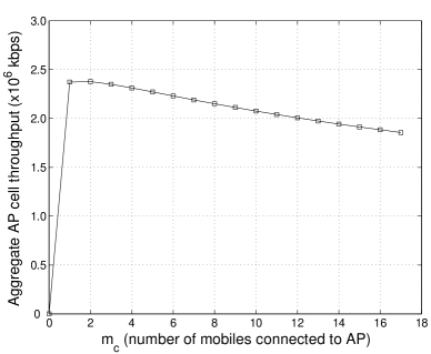
Figure 1: Total throughput of all mobiles in an AP cell

2.3 Downlink Throughput in 802.11 WLAN AP

We reuse the downlink TCP throughput formula for a mobile in a WLAN from [16]. For completeness, here we briefly mention the network model that has been extensively studied in [16] and then simply restate the throughput expression without going into much details. Each mobile connected to the AP uses the Distributed Coordination Function (DCF) protocol with an RTS/CTS frame exchange before any data-ack frame exchange and each mobile has an equal probability of the channel being allocated to it. With the assumption of $W^{*}$ being set to $1$ (Section 2.2) any mobile will always have a TCP ack waiting to be sent back to the AP with probability $1/2$, which is also the probability that it contends for the channel. This is however true only for those versions of TCP that do not use delayed acks. If the AP is always saturated or backlogged, the average number of backlogged mobiles contending for the channel is given by $m_{b}=1+\frac{m_{c}}{2}$. Based on this assumption and since for any connection an ack is sent by the mobile for every TCP packet received, the downlink TCP throughput of a single mobile is given by Section 3.2 in [16] as,

$$\theta_{AP}(m_{c})=\frac{L_{TCP}}{m_{c}(T_{TCPdata}+T_{TCPack}+2T_{tbo}+2T_{w})},$$ (1)

where $L_{TCP}$ is the size of TCP packets and $T_{TCPdata}$ and $T_{TCPack}$ are the raw transmission times of a TCP data and a TCP ack packet, respectively. $T_{tbo}$ and $T_{w}$ denote the mean total time spent in back-off and the average total time wasted in collisions for any successful packet transmission and are computed assuming $m_{b}$ backlogged mobiles. The explicit expressions for $T_{TCPdata}$, $T_{TCPack}$, $T_{tbo}$ and $T_{w}$ can be referred to in [16]. However, we mention here that they depend on certain quantities whose numerical values have been provided in Section 3. Note that all mobiles connected to the AP achieve equal downlink TCP throughputs in a fair manner, given by Equation 1. Figure 1 shows a plot of total cell throughput in an AP cell. Since the total throughput monotonically decreases with increasing number of mobiles, the pole capacity of an AP cell $M_{AP}$ is limited by the QoS requirement $\theta_{min}$ bps of each mobile.

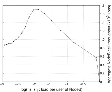
Figure 2: Total throughput of all mobiles in NodeB cell

2.4 Downlink Throughput in 3G-UMTS NodeB

We consider a standard model for data transmission on downlink in a 3G-UMTS NodeB cell. Let $W$ be the WCDMA modulation bandwidth and if $SINR$ denotes the signal to interference plus noise ratio received at a mobile then its energy per bit to noise density ratio is given by,

$$\frac{E_{b}}{N_{o}}=\frac{W}{\theta_{3G}}\times SINR.$$ (2)

Now, under the assumptions of identical throughput allocation to each mobile arriving at an average location and application of power control so that each mobile receives the same SINR (Section 2.2), we deduce from Eq. 2 that each mobile requires the same $E_{b}/N_{o}$ ratio in order to be able to successfully decode NodeB’s transmission. From Chapter 8 in [12] we can thus say that the downlink TCP throughput $\theta_{3G}$ of any mobile, in a NodeB cell with saturated resource allocation, as a function of load per user $\eta$ is given by,

$$\theta_{3G}(\eta)=\frac{\eta W}{(E_{b}/N_{o})(1-\bar{\alpha}+\bar{i})},$$ (3)

where $\bar{\alpha}$ and $\bar{i}$ have been defined before in Section 2.2. Figure 2 shows a plot of total cell throughput of all mobiles against $log(\eta)$ in a UMTS NodeB cell. The load per user $\eta$ has been stretched to a logarithmic scale for better presentation. Also note that throughput values have been plotted in the second quadrant. As we go away from origin on the horizontal axis, $log(\eta)$ (and $\eta$) decreases or equivalently number of connected mobiles increase. The equivalence between $\eta$ and $log(\eta)$ scales and number of mobiles $N(\eta)$ can be referred to in Table 1.

$$\begin{array}[]{||c|c|c||c||c||c||}\hline\cr\eta&log(\eta)&N(\eta)&SINR&\theta_{3G}&\frac{E_{b}}{N_{o}}\\ &&&(dB)&(kbps)&(dB)\\ \hline\cr 0.9&-0.10536&1&0.8423&572&9.0612\\ \hline\cr 0.45&-0.79851&2&-2.1804&465&6.9503\\ \hline\cr 0.3&-1.204&3&-3.7341&405&5.7894\\ \hline\cr 0.225&-1.4917&4&-5.1034&360&5.0515\\ \hline\cr 0.18&-1.7148&5&-6.0327&322&4.5669\\ \hline\cr 0.15&-1.8971&6&-6.5093&285&4.3052\\ \hline\cr 0.1286&-2.0513&7&-7.2075&242&4.3460\\ \hline\cr 0.1125&-2.1848&8&-8.8312&191&4.7939\\ \hline\cr 0.1&-2.3026&9&-8.9641&144&5.5091\\ \hline\cr 0.09&-2.4079&10&-9.1832&115&6.0281\\ \hline\cr 0.0818&-2.5033&11&-9.9324&96&6.3985\\ \hline\cr 0.0750&-2.5903&12&-10.1847&83&6.6525\\ \hline\cr 0.0692&-2.6703&13&-10.7294&73&6.8625\\ \hline\cr 0.0643&-2.7444&14&-10.9023&65&7.0447\\ \hline\cr 0.06&-2.8134&15&-10.9983&60&7.0927\\ \hline\cr 0.0563&-2.8779&16&-11.1832&55&7.1903\\ \hline\cr 0.0529&-2.9386&17&-11.3802&51&7.2549\\ \hline\cr 0.05&-2.9957&18&-11.9231&47&7.3614\\ \hline\cr\end{array}$$

Table 1:

It is to be noted here that the required $E_{b}/N_{o}$ ratio by each mobile is a function of its throughput. Also, if the NodeB cell is fully loaded with $\eta_{DL}=\eta^{max}_{DL}$ and if each mobile operates at its minimum throughput requirement of $\theta_{min}$ then we can easily compute the pole capacity $M_{3G}$ of the cell as,

$$M_{3G}=\frac{\eta^{max}_{DL}W}{\theta_{min}(E_{b}/N_{o})(1-\bar{\alpha}+\bar{i})}.$$ (4)

For $\eta^{max}_{DL}=0.9$ and a typical NodeB cell scenario that employs the closed-loop fast power control mechanism mentioned previously in Section 2.2, Table 1 shows the SINR (fourth column) received at each mobile as a function of the avg. load per user (first column). Note that we consider a maximum cell load of $0.9$ and not $1$ in order to avoid instability conditions in the cell. These values of SINR have been obtained from radio layer simulations of a NodeB cell. The values shown here have been slightly modified since the original values are part of a confidential internal document at France Telecom R&D. The fifth column shows the downlink throughput with a block error rate (BLER) of $10^{-2}$ that can be achieved by each mobile as a function of the SINR observed at that mobile. And the sixth column in the table lists the corresponding values of $E_{b}/N_{o}$ ratio (obtained from Equation 2), that are required at each mobile to successfully decode NodeB’s transmission.

Figure 3: Hybrid cell scenario under Global optimality

3 Global Optimality: SMDP control formulation

In the Global Optimality approach, it is the network operator that takes the optimal decision for each mobile as to which of the two AP or NodeB networks the mobile will connect to, after it has been admitted into the hybrid cell by the CAC controller (Figure 3). Since decisions have to be made at each arrival, this gives an SMDP structure to the decision problem and we state the equivalent SMDP problem as follows:

• States: The state of a hybrid cell system is denoted by the tuple $(m_{c},\eta)$ where $m_{c}$ $(0\leq m_{c}\leq M_{AP})$ denotes the number of mobiles connected to the AP and $\eta$ $(0.05\leq\eta\leq 0.9)$ is the load per user of the NodeB cell.

• Events: We consider two distinguishable events: (i) arrival of a new mobile after it has been admitted by CAC and (ii) departure of a mobile after service completion.

• Decisions: For mobiles arriving in the common stream a decision action $a\in\{0,1,2\}$ has to be taken. $a=0$ represents rejecting the mobile, $a=1$ represents routing the mobile connection to AP network and $a=2$ represents routing the mobile connection to NodeB network.

• Rewards: Whenever a new incoming mobile is either rejected or routed to one of the two networks, it generates a certain state dependent reward. Generally, the aggregate throughput of an AP or NodeB cell drops when an additional new mobile connects to it. However the network operator gains some financial revenue from the mobile user at the same time. There is thus a trade-off between revenue gain and the aggregate network throughput which motivates us to formulate the reward as follows. The reward consists of the sum of a fixed financial revenue price component and $\beta$ times an aggregate network throughput component, where $\beta$ is an appropriate proportionality constant. When a mobile of the dedicated arrival streams is routed to the corresponding AP or NodeB, it generates a financial revenue of $f_{AP}$ and $f_{3G}$, respectively. A mobile of the common stream generates a financial revenue of $f_{AP3G\to AP}$ on being routed to the AP and $f_{AP3G\to 3G}$ on being routed to the NodeB. Any mobile that is rejected does not generate any financial revenue. The throughput component of the reward is represented by the aggregate network throughput of the corresponding AP or NodeB network to which a newly arrived mobile connects, taking into account the change in the state of the system caused by this new mobile’s connection. Whereas, if a newly arrived mobile in a dedicated stream is rejected then the throughput component represents the aggregate network throughput of the corresponding AP or NodeB network, taking into account the unchanged state of the system. For a rejected mobile belonging to the common stream, it is the maximum of the aggregate network throughputs of the two networks that is considered.

• Criterion: The optimality criterion is to maximize the total expected discounted reward over an infinite horizon and obtain a deterministic and stationary optimal policy.

Note that in the SMDP problem statement above, state transition probabilities have not been mentioned because depending on the action taken, the system moves into a unique new state deterministically, i.e., w.p. 1. For instance when action $a=1$ is taken, the state evolves from $(m_{c},\eta)$ to $(m_{c}+1,\eta)$ or when action $a=2$ is taken, the state evolves from $(m_{c},\eta)$ to $(m_{c},\eta-\Delta(\eta))$. Applying the well-known uniformization technique from [17], we can say that events (i.e., arrival or departure of mobiles) occur at the jump times of the combined Poisson process of all types of events with rate $\Lambda:=\lambda_{AP}+\lambda_{3G}+\lambda_{AP3G}+{\check{\mu}}_{AP}+{\check{\mu}}_{3G}$, where ${\check{\mu}}_{AP}:=\max_{m_{c}}{\mu_{AP}(m_{c})}$ and ${\check{\mu}}_{3G}:=\max_{\eta}{\mu_{3G}(\eta)}$. The departure of a mobile is either a real departure, or an artificial departure, when from a single mobile’s point of view the corresponding server slows down due to large number of mobiles in the network. Then, any event occurring, corresponds to an arrival on the dedicated streams with probability $\lambda_{AP}/\Lambda$ and $\lambda_{3G}/\Lambda$, an arrival on the common stream with probability $\lambda_{AP3G}/\Lambda$ and a real departure with probability $\mu_{AP}(m_{c})/\Lambda$ or $\mu_{3G}(\eta)/\Lambda$. As a result, the time periods between consecutive events are i.i.d. distributed and we can consider an $n-$stage SMDP decision problem. Let $V_{n}(m_{c},\eta)$ denote the maximum expected $n-$stage discounted reward for the hybrid cell, when the system is in state $(m_{c},\eta)$. The stationary optimal policy that achieves the maximum total expected discounted reward over an infinite horizon can then be obtained as a solution of the $n-$stage problem as $n\to\infty$. The discount factor is denoted by $\gamma$ ($0<\gamma<1$) and determines the relative worth of the present reward v/s the future rewards. State $(m_{c},\eta)$ of the system is observed right after the occurrence of an event, for example, right after a newly arriving mobile in the common stream has been routed to one of the networks, or right after the departure of a mobile. Let $U_{n}(m_{c},\eta;a)$ denote the maximum expected $n-$stage discounted reward for the hybrid cell when the system is in state $(m_{c},\eta)$, given that an arrival event has occurred and given that action ’$a$’ will be taken for this newly arrived mobile. We can then write down the following recursive Dynamic Programming (DP) equation to solve our SMDP decision problem. $\forall n\geq 0$ and $0\leq m_{c}\leq M_{AP}$, $0.05\leq\eta\leq 0.9$,

$$\begin{split}V_{n+1}(m_{c},\eta)&=\frac{\lambda_{AP}}{\Lambda}\max_{a\in\{0,1\}}\left\{R_{AP}(m_{c},\eta;a)+\gamma U_{n}(m_{c},\eta;a)\right\}\\ &\quad+\frac{\lambda_{3G}}{\Lambda}\max_{a\in\{0,2\}}\left\{R_{3G}(m_{c},\eta;a)+\gamma U_{n}(m_{c},\eta;a)\right\}\\ &\quad+\frac{\lambda_{AP3G}}{\Lambda}\max_{a\in\{0,1,2\}}\left\{R_{AP3G}(m_{c},\eta;a)+\gamma U_{n}(m_{c},\eta;a)\right\}\\ &\quad+\frac{\mu_{AP}(m_{c})}{\Lambda}\gamma V_{n}((m_{c}-1)\vee 0,\eta)\\ &\quad+\frac{\mu_{3G}(\eta)}{\Lambda}\gamma V_{n}(m_{c},(\eta+\Delta(\eta))\wedge 0.9)\\ &\quad+\frac{\Lambda-(\lambda_{AP}+\lambda_{3G}+\lambda_{AP3G}+\mu_{AP}(m_{c})+\mu_{3G}(\eta))}{\Lambda}\gamma V_{n}(m_{c},\eta),\\ \end{split}$$ (5)

where,

$$\begin{split}R_{AP}(m_{c},\eta;a)&=\left\{\begin{array}[]{cc}\beta\;m_{c}\;\theta_{AP}(m_{c})&\;\;:a=0\\ f_{AP}+\beta\;(m_{c}+1)\;\theta_{AP}(m_{c}+1)&\;\;:a=1,m_{c}<M_{AP}\\ \beta\;m_{c}\;\theta_{AP}(m_{c})&\;\;:a=1,m_{c}=M_{AP}\end{array}\right.\end{split}$$ (6)

$$\begin{split}\hskip 7.11317ptR_{3G}(m_{c},\eta;a)&=\left\{\begin{array}[]{cc}\beta\;N(\eta)\;\theta_{3G}(\eta)&\;\;:a=0\\ f_{3G}+\beta\;N(\eta-\Delta(\eta))\;\theta_{3G}(\eta-\Delta(\eta))&\;\;:a=2,N(\eta)<M_{3G}\\ \beta\;N(\eta)\;\theta_{3G}(\eta)&\;\;:a=2,N(\eta)=M_{3G}\end{array}\right.\end{split}$$ (7)

$$\begin{split}R_{AP3G}(m_{c},\eta;a)&=\left\{\begin{array}[]{cc}\max\{\beta\;m_{c}\;\theta_{AP}(m_{c}),\beta\;N(\eta)\;\theta_{3G}(\eta)\}&\;\;:a=0\\ f_{AP3G\to AP}+\beta\;(m_{c}+1)\;\theta_{AP}(m_{c}+1)&\;\;:a=1,m_{c}<M_{AP}\\ \beta\;m_{c}\;\theta_{AP}(m_{c})&\;\;:a=1,m_{c}=M_{AP}\\ f_{AP3G\to 3G}+\beta\;N(\eta-\Delta(\eta))\;\theta_{3G}(\eta-\Delta(\eta))&\hskip 7.11317pt\;\;:a=2,N(\eta)<M_{3G}\\ \beta\;N(\eta)\;\theta_{3G}(\eta)&\hskip 7.11317pt\;\;:a=2,N(\eta)=M_{3G}\end{array}\right.\end{split}$$ (8)

and $U_{n}(m_{c},\eta;0):=V_{n}(m_{c},\eta)$, $U_{n}(m_{c},\eta;1):=V_{n}((m_{c}+1)\wedge M_{AP},\eta)$, $U_{n}(m_{c},\eta;2):=V_{n}(m_{c},(\eta-\Delta(\eta))\vee 0.05)$ for $\theta_{min}=46$ kbps and $N(\eta)$ can be obtained from Table 1. We solve the above DP equation with Value Iteration method using the following numerical values for various entities: $L_{TCP}=8000$ bits (size of TCP packets), $L_{MAC}=272$ bits, $L_{IPH}=320$ bits (size of MAC and TCP/IP headers), $L_{ACK}=112$ bits (size of MAC layer ACK), $L_{RTS}=180$ bits, $L_{CTS}=112$ bits (size of RTS and CTS frames), $R_{data}=11$ Mbits/s, $R_{control}=2$ Mbits/s (802.11 data transmission and control rates), $CW_{min}=32$ (minimum 802.11 contention window), $T_{P}=144\mu s$, $T_{PHY}=48\mu s$ (times to transmit the PLCP preamble and PHY layer header), $T_{DIFS}=50\mu s$, $T_{SIFS}=10\mu s$ (distributed inter-frame spacing time and short inter-frame spacing time), $T_{slot}=20\mu s$ (slot size time), $K=7$ (retry limit in 802.11 standard), $b_{0}=16$ (initial mean back-off), $p=2$ (exponential back-off multiplier), $\gamma=0.8$, $\lambda_{AP}=0.03$, $\lambda_{3G}=0.03$, $\lambda_{AP3G}=0.01$, $\zeta=10^{-6}$, $\beta=10^{-6}$, $M_{AP}=18$ and $M_{3G}=18$ for $\theta_{min}=46$ kbps, $\bar{\alpha}=0.9$ for ITU Pedestrian A channel, $\bar{i}=0.7$, $W=3.84$ Mcps and other values as illustrated in Table 1.

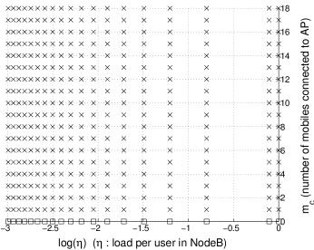
Figure 7: Optimal policy for AP dedicated flow in AP-NodeB hybrid cell

The DP equation has been solved for three different kinds of network setups. We first study the simple homogenous network case where both networks are AP and hence an incoming mobile belonging to the common stream must be offered a connection choice between two identical AP networks. Next, we study an analogous case where both networks are NodeB terminals. We study these two cases in order to gain some insight into connection routing dynamics in simple homogenous network setups before studying the third more complex, hybrid AP-NodeB scenario. Figures 6-8 show the optimal connection routing policy for the three network setups. Note that the plot in Figure 6 is in the $3^{rd}$ quadrant and plots in Figures 6-8 are in the $2^{nd}$ quadrant. In all these figures a square box symbol ($\Box$) denotes routing a mobile’s connection to the first network, a star symbol ($\ast$) denotes routing to the second network and a cross symbol ($\times$) denotes rejecting a mobile all together.

In Figure 6, optimal policy for the common stream in an AP-AP homogenous network setup is shown with $f_{AP1AP2\to AP1}=f_{AP1AP2\to AP2}=5$ (with some abuse of notation). The optimal policy routes mobiles of common stream to the network which has lesser number of mobiles than the other one. We refer to this behavior as mobile-balancing network phenomenon. This happens because the total throughput of an AP network decreases with increasing number of mobiles (Figure 1). Therefore, an AP network with higher number of mobiles offers lesser reward in terms of network throughput and a mobile generates greater incentive by joining the network with fewer mobiles. Also note that the optimal routing policy in this case is symmetric and of threshold type with the threshold switching curve being the coordinate line $y=x$.

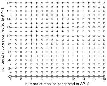
Figure 4: Optimal policy for common flow in AP-AP setup. First network: AP1, Second Network: AP2.

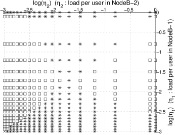
Figure 5: Optimal policy for common flow in NodeB-NodeB setup. First network: NodeB1, Second Network: NodeB2.

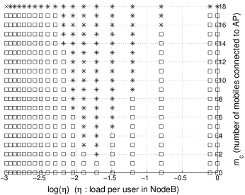
Figure 6: Optimal policy for common flow in AP-NodeB hybrid cell. First network: AP, Second Network: NodeB.

Figure 6 shows the optimal routing policy for the common stream in a NodeB-NodeB homogenous network setup. With equal financial incentives for the mobiles, i.e., $f_{3G13G2\to 3G1}=f_{3G13G2\to 3G2}=5$ (with some abuse of notation), we observe a very interesting switching curve structure. The state space in Figure 6 is divided into an L-shaped region (at bottom-left) and a quadrilateral shaped region (at top-right) under the optimal policy. Each region separately, is symmetric around the coordinate diagonal line $y=x$. With some abuse of notation, consider the state $(\eta_{1},\eta_{2})=(-0.79851,-1.4917)$ (not the coordinate point) of the homogenous network on logarithmic scale in the upper triangle of the quadrilateral region. From Table 1 this corresponds to the network state when load per user in the first NodeB network is $0.45$ which is more than the load per user of $0.225$ in the second NodeB network. Equivalently, there are less mobiles connected to the first network as compared to the second network. Ideally, one would expect new mobiles to be routed to the first network rather than the second network. However, according to Figure 6, in this state the optimal policy is to route to the second network even though the number of mobiles connected to it is more than those in the first. We refer to this behavior as mobile-greedy network phenomenon and explain the intuition behind it in the following paragraph. The routing policies on boundary coordinate lines are clearly comprehensible. On $y=-2.9957$ line when the first network is full (i.e., with least possible load per user), incoming mobiles are routed to second network (if possible) and vice-versa for the line $x=-2.9957$. When both networks are full, incoming mobiles are rejected which is indicated by the cross at coordinate point $(x,y)=(-2.9957,-2.9957)$.

The reason behind the mobile-greedy phenomenon in Figure 6 can be attributed to the fact that in a NodeB network, the total throughput increases with decreasing avg. load per user up to a particular threshold (say $\eta_{thres}$) and then decreases thereafter (see Figure 2). Therefore, routing new mobiles to a network with lesser (but greater than $\eta_{thres}$) load per user results in a higher reward in terms of total network throughput, than routing new mobiles to the other network with greater load per user. However, the mobile-greedy phenomenon is only limited to the quadrilateral shaped region. In the L-shaped region, the throughput of a NodeB network decreases with decreasing load per user, contrary to the quadrilateral region where the throughput increases with decreasing load per user. Hence, in the L-shaped region higher reward is obtained by routing to the network having higher load per user (lesser number of mobiles) than by routing to the network with lesser load per user (greater number of mobiles). In this sense the L-shaped region shows similar characteristics to mobile-balancing phenomenon observed in AP-AP network setup (Figure 6).

We finally discuss the hybrid AP-NodeB network setup. Here we consider financial revenue gains of $f_{AP3G\to AP}=5$ and $f_{AP3G\to 3G}=5.65$, motivated by the fact that a network operator can charge more for a UMTS connection since it offers a larger coverage area and moreover UMTS equipment is more expensive to install and maintain than WLAN equipment. In Figure 6, we observe that the state space is divided into two regions by the optimal policy switching curve which is neither convex nor concave. Moreover, in some regions of state space the mobile-balancing network phenomenon is observed, where as in some other regions the mobile-greedy network phenomenon is observed. In some sense, this can be attributed to the symmetric threshold type switching curve and the symmetric L-shaped and quadrilateral shaped regions in the corresponding AP-AP and NodeB-NodeB homogenous network setups, respectively. Figures 8 and 8 show the optimal policies for dedicated streams in an AP-NodeB hybrid cell with $f_{AP}=f_{3G}=0$. The optimal policy accepts new mobiles in the AP network only when there are none already connected. This happens because the network throughput of an AP is zero when there are no mobiles connected and a non-zero reward is obtained by accepting a mobile. Thereafter, since $f_{AP}=0$ the policy rejects all incoming mobiles due to decrease in network throughput and hence decrease in corresponding reward, with increasing number of mobiles. Similarly, for the dedicated mobiles to the NodeB network, the optimal policy accepts new mobiles until the network throughput increases (Figure 2) and rejects them thereafter due to absence of any financial reward component and decrease in the network throughput. Note that we have considered zero financial gains here ($f_{AP}=f_{3G}=0$) to be able to exhibit existence of these threshold type policies for the dedicated streams.

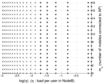
Figure 8: Optimal policy for NodeB dedicated flow in AP-NodeB hybrid cell

\psfrag{ETA}{$\eta$}\psfrag{MUC}{$m_{c}$}\psfrag{INN}{$\in$}\psfrag{TOO}{$\to$}\psfrag{PII}{$\pi$}\psfrag{TAU}{$\tau$}\includegraphics[width=209.58255pt]{figs/hybrid-net-indiv}

Figure 9: Hybrid cell scenario under Individual optimality

4 Individual Optimality: Non-cooperative Dynamic Game

In the Individual Optimality approach here, we assume that an arriving mobile must itself selfishly decide to join one of the two networks such that its own cost is optimized. We consider the average service time of a mobile as the decision cost criteria and an incoming mobile connects to either the AP or NodeB network depending on which of them offers minimum average service time. We study this model within an extension of the framework of [18] where an incoming user can either join a shared server with a PS service mechanism or any of several dedicated servers. Based on the estimate of its expected service time on either of the two servers, a mobile takes a decision to join the server on which its expected service time is least. This framework can be applied to our hybrid cell scenario so that the AP is modeled by the shared server and the dedicated DCH channels of the NodeB are modeled by the dedicated servers. For simplicity, we refer to the several dedicated servers in [18] as one single dedicated server that consists of a pool of dedicated servers. Then the NodeB comprising the dedicated DCH channels is modeled by this single dedicated server and this type of framework then fits well with our original setting in Section 2.1. Thus we again have an $M/G/2$ processing server situation (see Figure 9). As mentioned before, the mobiles of dedicated streams directly join their respective AP or NodeB network. Mobiles arriving in the common stream decide to join one of the two networks based on their estimate of the expected service time in each one of them. However, an estimate of the expected service time of an arriving mobile $j$ must be made taking into account the effect of subsequently arriving mobiles. But these subsequently arriving mobiles are themselves faced with a similar decision problem and hence their decision will affect the performance of mobile $j$ which is presently attempting to connect or other mobiles already in service. This dependance thus induces a non-cooperative game structure to the decision problem and we seek here to study the Nash equilibrium solution of the game. The existence, uniqueness and structure of the equilibrium point have been proved in [18] already. Here we seek to analytically determine the service time estimate and explicitly compute the equilibrium threshold policy. As in [18], a decision rule or policy for a new mobile is a function $u:\{0,1,\ldots,M_{AP}-1\}\rightarrow[0,1]$ where $M_{AP}$ is the pole capacity of the AP network. Thus for each possible state of the AP network denoted by number of mobiles already connected, $m_{c}$, a new mobile takes a randomized decision $u(m_{c})\in[0,1]$, that specifies the probability of connecting to the AP. $1-u(m_{c})$ then represents either the probability of connecting to the NodeB or abandoning to seek a connection altogether if both networks are full to their pole capacity. A policy profile $\pi=(u_{0},u_{1},\ldots)$ is a collection of decision rules followed by all arriving mobiles indexed $(0,1,\ldots)$.

Define $V_{AP}(m_{c},\pi)$ as the expected service time of a mobile in the AP network, given that it joins that network, $m_{c}$ mobiles are already present and all subsequent mobiles follow the policy profile $\pi$. A single mobile generally achieves lower throughputs (i.e., higher service times) in a NodeB network as compared to in an AP network. For simplification, we assume a worst case estimate for the expected service time of a mobile in the NodeB network. Denote ${\hat{\mu}}_{3G}:=\min_{\eta}{\mu_{3G}(\eta)}$ and let $\tau:=1/{\hat{\mu}}_{3G}$ be the maximum service time of a mobile in the NodeB cell, which is independent of network state $\eta$. For some $q$ ($0\leq q\leq 1$, $q\in\mathbb{R}$), define a decision policy $u(m_{c})$ to be the best response of a new mobile, against the policy profile $\pi=(u_{0},u_{1},\ldots)$ followed by all subsequently arriving mobiles [18], as,

$$u(m_{c})=\left\{\begin{array}[]{cc}1&\qquad:\;V_{AP}(m_{c},\pi)<\tau\\ q&\qquad:\;V_{AP}(m_{c},\pi)=\tau\\ 0&\qquad:\;V_{AP}(m_{c},\pi)>\tau\end{array}\right.$$

Further, define a special kind of decision policy, namely the threshold policy as, given $q$ and $L$ such that $0\leq q\leq 1$, $q\in\mathbb{R}$ and $L\geq 0$, $L\in\mathbb{Z}^{+}$, an $L,q$ threshold policy $u_{L,q}$ is defined as,

$$u_{L,q}(m_{c})=\left\{\begin{array}[]{cc}1&\qquad:\;m_{c}<L\\ q&\qquad:\;m_{c}=L\\ 0&\qquad:\;m_{c}>L\end{array}\right.$$

This $L,q$ threshold policy will be denoted by $[L,q]$ or more compactly by $[g]$ where $g=L+q$. Note that the threshold policies $[L,1]$ and $[L+1,0]$ are identical. We also use the notation ${[g]}^{\infty}\equiv{[L,q]}^{\infty}$ to denote the policy profile $\pi=([g],[g],\ldots)$. Now, it has been proved in Lemma 3 in [18] that the optimal best response decision policy $u(m_{c})$ for a new mobile, against the policy profile $\pi$ followed by all subsequently arriving mobiles, is actually the threshold policy $[L^{*},q^{*}]$ which can be computed as follows. If $V_{AP}(M_{AP}-1,{[M_{AP}]}^{\infty})<\tau$ then $L^{*}=M_{AP}$ and $q^{*}=0$. Otherwise, let $L^{min}\stackrel{{\scriptstyle\Delta}}{{=}}\min\{L\in\mathbb{Z}^{+}:V_{AP}(L,{[L,1]}^{\infty})>\tau\}$. Now, if $V_{AP}(L^{min},[L^{min},0]^{\infty})\geq\tau$, then the threshold policy is given by $[L^{*},q^{*}]=[L^{min},0]$. Else if $V_{AP}(L^{min},[L^{min},0]^{\infty})<\tau$ then it is given by $[L^{*},q^{*}]=[L^{min},q^{*}]$ where $q^{*}$ is the unique solution of the equation,

$$V_{AP}(L^{min},[L^{min},q^{*}]^{\infty})=\tau.$$ (9)

Assuming state dependent service rate $\mu_{AP}(m_{c})$ for a mobile in the AP network, we now compute $V_{AP}(m_{c},\pi)$ analytically. At this point we would like to mention that the derivation of the entity equivalent to $V_{AP}(m_{c},\pi)$ in [18] is actually erroneous. Moreover the basic framework in [18] differs from ours, since in our framework we have dedicated arrivals in addition to the common arrivals and we consider a state dependent service rate $\mu_{AP}(m_{c})$ for the shared AP server. For notational convenience, if $V(m_{c})\stackrel{{\scriptstyle\Delta}}{{=}}V_{AP}(m_{c},[L,q]^{\infty}),0\leq m_{c}\leq M_{AP}-1$, then it is the solution of the following set of $M_{AP}$ linear equations, where $\alpha:=\lambda_{AP}+\lambda_{AP3G}+\mu_{AP}(m_{c})$ (dependence of $\alpha$ on $m_{c}$ has been suppressed in the notation):

Case 1: $4\leq L\leq M_{AP}-2$,

$$\begin{split}V(0)&=\frac{1}{\alpha}+\frac{\lambda_{AP}+\lambda_{AP3G}}{\alpha}V(1)\\ V(m_{c})&=\frac{1}{\alpha}+\frac{\mu_{AP}(m_{c})}{\alpha}\frac{m_{c}}{m_{c}+1}V(m_{c}-1)+\frac{\lambda_{AP}+\lambda_{AP3G}}{\alpha}V(m_{c}+1),\\ &\hskip 256.0748pt1\leq m_{c}\leq L-2\\ V(L-1)&=\frac{1}{\alpha}+\frac{\mu_{AP}(L-1)}{\alpha}\frac{L-1}{L}V(L-2)+\frac{\lambda_{AP}+q\;\lambda_{AP3G}}{\alpha}V(L)\\ &\quad+\frac{\lambda_{AP3G}}{\alpha}(1-q)V(L-1)\\ V(L)&=\frac{1}{\lambda_{AP}+\mu_{AP}(L)}+\frac{\mu_{AP}(L)}{\lambda_{AP}+\mu_{AP}(L)}\frac{L}{L+1}V(L-1)+\frac{\lambda_{AP}}{\lambda_{AP}+\mu_{AP}(L)}V(L+1)\\ V(m_{c})&=\frac{1}{\lambda_{AP}+\mu_{AP}(m_{c})}+\frac{\mu_{AP}(m_{c})}{\lambda_{AP}+\mu_{AP}(m_{c})}\frac{m_{c}}{m_{c}+1}\\ &\quad\times V(m_{c}-1)+\frac{\lambda_{AP}}{\lambda_{AP}+\mu_{AP}(m_{c})}V(m_{c}+1),\quad L+1\leq m_{c}\leq M_{AP}-2\\ V(M_{AP}-1)&=\frac{1}{\mu_{AP}(M_{AP}-1)}+\frac{M_{AP}-1}{M_{AP}}V(M_{AP}-2)\end{split}$$ (10)

Case 2: $L=M_{AP}-1$,

$$\begin{split}V(0)&=\frac{1}{\alpha}+\frac{\lambda_{AP}+\lambda_{AP3G}}{\alpha}V(1)\\ V(m_{c})&=\frac{1}{\alpha}+\frac{\mu_{AP}(m_{c})}{\alpha}\frac{m_{c}}{m_{c}+1}V(m_{c}-1)+\frac{\lambda_{AP}+\lambda_{AP3G}}{\alpha}V(m_{c}+1),\quad 1\leq m_{c}\leq L-2\\ V(L-1)&=\frac{1}{\alpha}+\frac{\mu_{AP}(L-1)}{\alpha}\frac{L-1}{L}V(L-2)+\frac{\lambda_{AP}+q\;\lambda_{AP3G}}{\alpha}V(L)\\ &\quad+\frac{\lambda_{AP3G}}{\alpha}(1-q)V(L-1)\\ V(L)&=\frac{1}{\mu_{AP}(L)}+\frac{L}{L+1}V(L-1).\end{split}$$ (11)

The above system of $M_{AP}$ linear equations with $m_{c}=L$ and $q=1$ can be solved to obtain $V_{AP}(L,[L,1]^{\infty})$ for different values of $L$. Figure 10 shows an example plot for $\zeta=10^{-5}$, $\lambda_{AP}=3$, $M_{AP}=10$, $M_{3G}=10$ and other numerical values for various entities in WLAN and UMTS networks being the same as those used in Section 3. Assuming a certain pole capacity $M_{3G}$ of the NodeB cell, $\tau$ can be computed from its definition and Equation 4. Knowing $\tau$, one can compute $L^{min}$ from Figure 10 and then finally $q^{*}$ from Equation 9. Figure 11 shows a plot of the equilibrium threshold $g^{*}=L^{*}+q^{*}$ against $\lambda_{AP3G}$, with computed value of $\tau=2.5$ for $M_{3G}=10$ and $\lambda_{AP}=3$. As in [18], the equilibrium threshold has a special structure of descending staircase with increasing arrival rate ($\lambda_{AP3G}$) of mobiles in common stream.

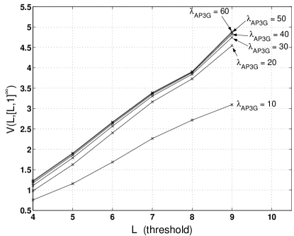
Figure 10: $V_{AP}(L,[L,1]^{\infty})$ v/s $L$ for $\lambda_{AP}=3$ and $M_{AP}=10$

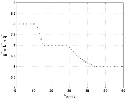
Figure 11: $g^{*}$ v/s $\lambda_{AP3G}$ for $\lambda_{AP}=3$, $M_{AP}=10$ and $\tau=2.5$

5 Conclusion

In this paper, we have considered optimal user-network association or load balancing in an AP-NodeB hybrid cell. We have studied two different and alternate approaches of Global and Individual optimality under SMDP decision control and non-cooperative dynamic game frameworks, respectively. To the best of our knowledge, this study is the first of its kind. Under global optimality, the optimal policy for common stream of mobiles has a neither convex nor concave type switching curve structure, where as for the dedicated streams it has a threshold structure. Besides, a mobile-balancing and a mobile-greedy network phenomenon is observed for the common stream. For the analogous AP-AP homogenous network setup, a threshold type and symmetric switching curve is observed. An interesting switching curve is obtained for the NodeB-NodeB homogenous case, where the state space is divided into L-shaped and quadrilateral shaped regions. The optimal policy under individual optimality model is also observed to be of threshold type, with the threshold curve decreasing in a staircase fashion when plotted against increasing arrival rate of the mobiles of common stream.

References

- [1] L. Ma, F. Yu, V.C. M. Leung, T. Randhawa, A New Method to support UMTS/WLAN Vertical Handover using SCTP, IEEE Wireless Commun., Vol.11, No.4, p.44-51, Aug. 2004.
- [2] J. Song, S. Lee, D. Cho, Hybrid Coupling Scheme for UMTS and Wireless LAN Interworking, Proc. VTC-Fall, Vol.4, pp.2247-2251, Oct. 2003.
- [3] C. Liu, C. Zhou, HCRAS: A Novel Hybrid Internetworking Architecture between WLAN and UMTS Cellular Networks, IEEE Consumer Communications and Networking conference, Las Vegas, Jan. 2005.
- [4] M. Jaseemuddin, An Architecture for integrating UMTS and 802.11 WLAN Networks, Proc. ISCC 2003, Turkey, July 2003.
- [5] N. Vulic, S. H. Groot, I. Niemegeers, Common Radio Resource Management for WLAN-UMTS Integration Radio Access Level, Proc. IST Mobile & Wireless Communications Summit 2005, Germany, June 2005.
- [6] H. Kwon, K. Rho, A. Park, J. Ryou, Mobility Management for UMTS-WLAN Seamless Handover: within the Framework of Subscriber Authentication Proc. ISATED Communication, Network and Information Security (CNIS), Nov. 2005.
- [7] O. E. Falowo, H. A. Chan, AAA and Mobility Management in UMTS-WLAN Interworking Proc. 12th International Conference on Telecommications (ICT), Cape Town, May 2005.
- [8] K. Premkumar, A. Kumar, Optimal Association of Mobile Wireless Devices with a WLAN-3G Access Network, Proc. IEEE ICC, June 2006.
- [9] F. Yu, V. Krishnamurthy, Efficient Radio Resource Management in Integrated WLAN/CDMA Mobile Networks, Telecommunication Systems Journal, Springer, Vol.30, No.1-3, p.177-192, Nov. 2005.
- [10] Fu et al., The Impact of Multihop Wireless Channel on TCP Throughput and Loss, Proc. IEEE INFOCOM, 2003.
- [11] F. Lebeugle, A. Proutiere, User-level performance in WLAN hotspots, Proc. ITC, Beijing, Sept. 2005.
- [12] H. Holma, A. Toskala, WCDMA for UMTS, Rev. Ed., Wiley, 2001.
- [13] L. Zan, G. Heijenk, M. E. Zarki, Fair & Power-Efficient Channel-Dependent Scheduling for CDMA Packet Nets., Proc. ICWN, USA, 2003.
- [14] A. Kumar, E. Altman, D. Miorandi and M. Goyal, New insights from a fixed point analysis of single cell IEEE 802.11 WLANs, Proc. IEEE Infocom, USA, March 2005.
- [15] T. Bonald, A score-based opportunistic scheduler for fading radio channels, Proc. European Wireless, 2004.
- [16] D. Miorandi, A. Kherani, E. Altman, A Queueing Model for HTTP Traffic over IEEE 802.11 WLANs, Computer Networks, Vol.50, Issue 1, p.63-79, Jan’06.
- [17] S. A. Lippman, Applying a new device in the optimization of exponential queueing systems, Operations Research, p.687-710, 1975.
- [18] E. Altman, N.Shimkin, Individual equilibrium and learning in a processor sharing system, Operations Research, Vol.46, p.776-784, 1998.