A Graph-based Framework for Transmission of Correlated Sources over Broadcast Channels

Abstract

In this paper we consider the communication problem that involves transmission of correlated sources over broadcast channels. We consider a graph-based framework for this information transmission problem. The system involves a source coding module and a channel coding module. In the source coding module, the sources are efficiently mapped into a nearly semi-regular bipartite graph, and in the channel coding module, the edges of this graph are reliably transmitted over a broadcast channel. We consider nearly semi-regular bipartite graphs as discrete interface between source coding and channel coding in this multiterminal setting. We provide an information-theoretic characterization of (1) the rate of exponential growth (as a function of the number of channel uses) of the size of the bipartite graphs whose edges can be reliably transmitted over a broadcast channel and (2) the rate of exponential growth (as a function of the number of source samples) of the size of the bipartite graphs which can reliably represent a pair of correlated sources to be transmitted over a broadcast channel.

1 Introduction

With the emergence of new set of applications such as wireless sensor networks, the problem of transmission of correlated information sources over multiterminal channels has received a renewed attention. In this problem, many correlated information sources are accessed by a set of transmitter terminals, and they wish to simultaneously transmit some subset of them to another set of receiver terminals over a channel. In this paper we address the one-to-many communication system, where one transmitter terminal has access to all the information sources, and wish to transmit them to many receiver terminals. One such model involving two receiver terminals was considered by Han and Costa in [1], and is described in the following. Consider a pair of correlated discrete memoryless sources $(S,T)$ with some generic joint distribution $p(s,t)$ and a pair of finite alphabets $\mathcal{S}$ and $\mathcal{T}$, respectively. The encoder observes long sequences of realizations of these sources (of length say $n$), and wishes to transmit them over a broadcast channel which has one input $X$ and two outputs $Y_{1}$ and $Y_{2}$, and Receiver i has access to $Y_{i}$. The channel behavior is governed by a generic conditional distribution $p(y_{1},y_{2}|x)$. The channel is assumed to be discrete memoryless and is used without feedback. The encoder maps $n$-length source sequence pairs into $n$-length channel input sequences. Each receiver maps its corresponding $n$-length channel output sequences into its corresponding $n$-length source reconstruction sequences. The receivers would like to produce a reconstruction sequence pair such that the probability that this deviates from the original pair goes to zero as blocklength $n$ becomes large. If it is possible to build such sequences of mappings, then we say that the source pair is transmissible over the broadcast channel. The goal is to find the set of all sources that are transmissible over a given broadcast channel or the set of all channels over which a given source pair is transmissible.

Two approaches have been proposed for this problem in the literature. On is called the joint-source-channel coding approach and the other is the separation-approach. The former approach [1] addresses the problem directly by finding the mappings for the given source pair and broadcast channel. A sufficient condition for transmissibility of a source over a channel has been given in [1] for this problem. In the separation-approach, we divide the encoding task into two sub-tasks, and similarly the decoding task is accomplished in two steps. In this approach, the $n$-length source pair is mapped into three indexes (referred to as $W_{0}$, $W_{1}$ and $W_{2}$) coming from three finite sets of size say $\Delta_{0}$, $\Delta_{1}$ and $\Delta_{2}$, respectively. The first index (common message) is meant for both receivers, and the second and the third indexes (private messages) are meant for Receiver 1 and Receiver 2, respectively. This is called source encoding. The goal is to remove all the redundancy from the pair to produce three independent bit streams. Then these three indexes are mapped (referred to as channel coding) to $n$-length channel input sequences. On the other side of the channel, Receiver i first maps its $n$-length channel output into a pair of indexes ($W_{0}$ and $W_{i}$) for $i=1,2$. Then they independently produce source reconstruction sequences from the common and the private messages. The first goal is to find the set (called as the rate region) of all the rate tuples $(R_{0},R_{1},R_{2})$, where $R_{j}=\frac{1}{n}\log\Delta_{j}$ for $j=0,1,2$, at which a reliable representation of the given source pair can be accomplished. The second goal is to find the set (called as the capacity region) of all rate tuples $(R_{0},R_{1},R_{2})$, at which a reliable communication of indexes over the given channel can be accomplished. The source coding part works under the assumption that the channel is noiseless, and the channel coding part works under the assumption that the messages are independent.

The channel coding part by itself was first introduced by Cover in [2, 3]. The capacity region has been found for many interesting classes of broadcast channels [2, 3, 4, 5, 6, 7, 8, 9, 10, 11, 12, 13, 14]. The capacity region of certain class of broadcast channels used in wireless communication systems have been obtained in [15, 16, 17, 18, 19, 20, 21]. Marton [12] (also see [22, 23, 24]) established an inner bound to the capacity region for the discrete memoryless broadcast channel, which contains all the known achievable rate regions. Outer bounds to the capacity region have been obtained in [25, 12, 26]. See [27] for a latest survey of the results on broadcast channels. The source coding part was addressed by Gray and Wyner in [28], where a complete characterization of the rate region was given. We refer this source coding problem as Gray-Wyner problem. However, it is well-known that the separation-approach is not optimal for the one-to-many communication problem, unlike the case of point-to-point information transmission problem. In particular, a simple example was given in [1] that showed that a triangular source can be sent reliably over a Blackwell channel by using a simple joint-source-channel coding scheme, but there is no way of transmitting that source over that channel using the separation-approach.

Loosely speaking, in the separation-approach, there is an interface between the source coding module and the channel coding module. Due to the structure of the system, i.e., a common message and a pair of private messages, the interface can be thought of as a finite collection of products of finite sets. For example, in a system with $\Delta_{i}$ denoting the size of the $i$th message for $i=0,1,2$, the interface can be thought of as $\cup_{i=1}^{\Delta_{0}}(A_{i}\times B_{i})$, where $A_{i}=\{(i-1)\Delta_{1}+1,(i-1)\Delta_{1}+2,\ldots,i\Delta_{1}\}$ and $B_{i}=\{(i-1)\Delta_{2}+1,(i-1)\Delta_{2}+2,\ldots,i\Delta_{2}\}$. However, as seen above, this interface, a finite collection of products of finite sets, is not an efficient representation of a pair of correlated sources for transmission over broadcast channels. Note that the corresponding interface for a similar approach in the point-to-point case is just a finite set. It is also well-known that a similar separation-approach is not optimal for other multiuser information transmission problems such as many-to-one communication [29].

In our recent work [30, 31], we have reported a bipartite graph-based framework for the problem of transmission of information in the many-to-one case. A similar approach was also studied in [32]. In the present work, we consider a similar approach to the one-to-many communication scenario. The fundamental motivation for this comes from the concept of typicality [33]. Given a correlated source pair $(S,T)$, a sequence in $\mathcal{S}^{n}$ is said to be typical (or individually typical) with respect to $p(s)$, if its empirical histogram is close to $p(s)$. Similarly one can define typical sequences in $\mathcal{T}^{n}$. A sequence pair in $\mathcal{S}^{n}\times\mathcal{T}^{n}$ is said to be jointly typical if its empirical joint histogram is close to $p(s,t)$. Using the law of large numbers, it follows that (a) there are roughly $2^{nH(S)}$ and $2^{nH(T)}$ individually typical sequences in $\mathcal{S}^{n}$ and $\mathcal{T}^{n}$, respectively, where $H(\cdot)$ denotes entropy [33], (b) there are roughly $2^{nH(S,T)}$ jointly typical sequence pairs in $\mathcal{S}^{n}\times\mathcal{T}^{n}$, (c) for every typical sequence in $\mathcal{S}^{n}$, there are roughly $2^{nH(T|S)}$ typical sequences in $\mathcal{T}^{n}$ that are jointly typical and vice versa, (d) probability, under $p(s,t)$, of the set of jointly typical sequences (called jointly typical set) is close to $1$, and (e) the probability, under $p(s,t)$, of every jointly typical sequence pair is roughly equal to $2^{-nH(S,T)}$. These five properties lead one to associate a bipartite graph on the jointly typical set, with vertexes formed by individually typical sequences, and two vertexes are connected by an edge if they are jointly typical. Such bipartite graphs, where the degrees of the vertexes of one set is close to one constant, and the degrees of that of the other set is close to another constant, are referred to as nearly semi-regular [34]. Hence graphs can naturally capture the behavior of the source pair. The details regarding the source distribution can be dispensed with, and one can just work with this bipartite graph. This may also lead to the possibility of using them as discrete interface for one-to-many communication. The source encoder would now act on the source pair and produce correlated messages, or edges in a bipartite graph, and the channel encoder would now work with correlated messages and reliably transmit the edges in the graph over the broadcast channel. We would still have a source coding module and a channel coding module. However, now they would be interfaced using nearly semi-regular bipartite graphs rather than just a finite collection of products of finite sets. Of course, a finite collection of products of finite sets is a special case of nearly semi-regular bipartite graphs.

We now present a brief summary of the results presented in this paper, for which we need some definitions. A nearly semi-regular bipartite graph is said to have parameters $(\theta_{1},\theta_{2},\theta^{\prime}_{1},\theta^{\prime}_{2})$ if the $i$th vertex set has size nearly equal to $\theta_{i}$ for $i=1,2$, and the degrees of vertexes of the first set is nearly equal to $\theta^{\prime}_{2}$ and vice versa. With a slight abuse of notation, a nearly semi-regular bipartite graph is said to have parameters $(\theta_{0},\theta_{1},\theta_{2},\theta^{\prime}_{1},\theta^{\prime}_{2})$ if it is the union of $\theta_{0}$ disjoint subgraphs each having parameters $(\theta_{1},\theta_{2},\theta^{\prime}_{1},\theta^{\prime}_{2})$. A tuple of rates $(R_{0},R_{1},R_{2},R^{\prime}_{1},R^{\prime}_{2})$ is said to be achievable for the given broadcast channel if there exists a bipartite graph with parameters $(2^{nR_{0}},2^{nR_{1}},2^{nR_{2}},2^{nR^{\prime}_{1}},2^{nR^{\prime}_{2}})$ whose edges can be reliably transmitted by using the channel $n$ times for large $n$. Similarly, a tuple of rates $(R_{0},R_{1},R_{2},R^{\prime}_{1},R^{\prime}_{2})$ is said to be achievable for a given pair of correlated sources if there exists a bipartite graph with parameters $(2^{nR_{0}},2^{nR_{1}},2^{nR_{2}},2^{nR^{\prime}_{1}},2^{nR^{\prime}_{2}})$ which can reliably represent $n$ realizations of the pair for large $n$. We provide information-theoretic partial characterizations of the sets of achievable tuples for a broadcast channel and a correlated source pair. These are presented in Theorem 1-4. Having the significance of the proposed framework mentioned first, let us look at the limitations of this optimistic framework as well. For that we need to look at the big picture.

For the point-to-point case, to check the transmissibility of a source over a channel, we just need to check the non-emptiness of the intersection of two intervals $[H,\infty)$ and $[0,C]$, where $H$ denotes the entropy of the source, and $C$ denotes the capacity of the channel. Note that only one parameter specifies the interval. For the one-to-many communication, the conventional separation-approach gives a sufficient condition for checking the transmissibility: non-emptiness of the rate region of the source pair and that of the broadcast channel. We need three parameters $(R_{0},R_{1},R_{2})$ to specify the rate region in both source coding as well as channel coding. Clearly, a characterization that involves the fewest number of parameters is what we want.

In the graph-based framework, we consider rate regions for the source and the channel, which are specified using five parameters: $(R_{0},R_{1},R_{2},R^{\prime}_{1},R^{\prime}_{2})$. However, the non-empty intersection of the rate region of the source pair with that of the channel still does not guarantee successful transmission. This is because, graphs having the same set of parameters may have different structures. It turns out that these graphs (that have the same set of parameters) can be partitioned into equivalence classes, where all graphs in an equivalence class have the same structure. This structure of the graphs has also been studied under the name of graph isomorphism [34] in the literature. We will address this issue more formally in later sections. Hence a graph with parameters (say) $(2^{nR_{0}},2^{nR_{1}},2^{nR_{2}},2^{nR^{\prime}_{1}},2^{nR^{\prime}_{2}})$ which can reliably represent a source pair may not belong to the equivalence class of a graph with the same set of parameters whose edges can be transmitted reliably over the channel. In other words, to guarantee successful transmission of the source over the channel, we need to construct at least one pair of transmission systems (one for the source component and one for the channel component) for every equivalence class. Rather, in this work we have shown (a) the existence of an equivalence class for which a transmission system could be built in the source coding component, and (b) the existence of an equivalence class for which a transmission system could be built in the channel coding component. We plan to address this issue further in our future work. But we believe that the results given in this paper may be a first step toward an optimal discrete interface for multiuser communication.

The outline of the remaining part of this paper is as follows. In Section 2, we first provide a summary of the results in a formal setting that are available in the literature that are closely related to our work. Then, in Section 3, we formulate the problem and consider certain properties of bipartite graphs that are relevant to our later discussion. Then channel coding part will be discussed in Section 4, resulting in an achievable rate region for the broadcast channel with correlated messages. We also consider the special case of broadcast channels with one deterministic component. Thereafter, the complementary source coding part, the representation of correlated sources into graphs, will be described in Section 5. After that, an example and its interpretation are provided in Section 6. Finally, Section 7 provides some concluding remarks.

2 Preliminaries

In this section, we provide an overview of the most important prior results in the literature on broadcast channels, and the related source coding problem, which are closely related to our work.

2.1 Broadcast Channel with Independent private Messages

A broadcast channel is composed of one sender and many receivers. The objective is to broadcast information from a sender to the many receivers. We consider broadcast channels with only two receivers since multiple receivers cases can be similarly treated. Figure 1 shows a broadcast channel with one sender and two receivers. The discrete memoryless stationary broadcast channel consists of an input alphabet $\mathcal{X}$ and two output alphabets $\mathcal{Y}_{1}$ and $\mathcal{Y}_{2}$ and a conditional distribution $p(y_{1},y_{2}|x)$. The induced $n$-length conditional distribution is given by $p(y_{1}^{n},y_{2}^{n}|x^{n})=\prod_{i=1}^{n}p(y_{1i},y_{2i}|x_{i})$ when used without feedback. In other words, a broadcast channel is an ordered tuple $(\mathcal{X},\mathcal{Y}_{1},\mathcal{Y}_{2},p(y_{1},y_{2}|x))$.

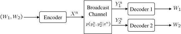
Figure 1: Broadcast channel

We consider the following definitions for transmission of independent messages over a broadcast channel.

Definition 1

A transmission system with parameters $(n,\Delta_{0},\Delta_{1},\Delta_{2},\tau)$ for the given broadcast channel $(\mathcal{X},\mathcal{Y}_{1},$ $\mathcal{Y}_{2},p(y_{1},y_{2}|x))$ is an ordered tuple $(f,g_{1},g_{2})$, consisting of one encoding mapping $f$ and two decoding mappings $g_{1}$ and $g_{2}$ where

• $f:\{1,2,\ldots,\Delta_{0}\}\times\{1,2,\ldots,\Delta_{1}\}\times\{1,2,\ldots,\Delta_{2}\}\rightarrow\mathcal{X}^{n}$,

• $g_{i}:\mathcal{Y}_{i}^{n}\rightarrow\{1,2,\ldots,\Delta_{0}\}\times\{1,2,\ldots,\Delta_{i}\}$, for $i=1,2$,

• such that a performance measure given by the average probability of error satisfies:

  $$\tau=\sum_{k=1}^{\Delta_{0}}\sum_{i=1}^{\Delta_{1}}\sum_{j=1}^{\Delta_{2}}\frac{1}{\Delta_{0}\Delta_{1}\Delta_{2}}Pr\left[(g_{1}(Y_{1}^{n}),g_{2}(Y_{2}^{n}))\neq((k,i),(k,j))|X^{n}=f(k,i,j)\right].$$

Definition 2

A rate tuple $(R_{0},R_{1},R_{2})$ is said to be achievable for the given broadcast channel if for all $\epsilon>0$, and for sufficiently large $n$, there exists a transmission system as defined above satisfying $\frac{1}{n}\log\Delta_{i}>R_{i}-\epsilon$ for $i=0,1,2$ and with the average probability of error $\tau<\epsilon$.

Definition 3

The capacity region $\mathcal{C}_{BCI}$ of the broadcast channel is the set of all achievable rate tuples $(R_{0},R_{1},R_{2})$.

The capacity region of general broadcast channels is still not known. But Marton [12] and Gelfand and Pinsker [13] have obtained an achievable rate region for the general discrete memoryless broadcast channel, which is the largest known inner bound to the capacity region. An achievable region of the discrete memoryless broadcast channel [35] is given by all rate tuples $(R_{0},R_{1},R_{2})$ satisfying

$$R_{0} <\min\{I(Z;Y_{1}),I(Z;Y_{2})\},$$ (1)

$$R_{0}+R_{1} <I(Z,U;Y_{1}),$$ (2)

$$R_{0}+R_{2} <I(Z,V;Y_{2}),$$ (3)

$$R_{0}+R_{1}+R_{2} <\min\{I(Z;Y_{1}),I(Z;Y_{2})\}+I(U;Y_{1}|Z)+I(V;Y_{2}|Z)-I(U;V|Z)$$ (4)

for some $p(z,u,v,x)$ on ${\mathcal{Z}}\times$ ${\mathcal{U}}\times{\mathcal{V}}\times{\mathcal{X}}$, where $Z$, $U$ and $V$ are auxiliary random variables with finite alphabets ${\mathcal{Z}}$, ${\mathcal{U}}$, and ${\mathcal{V}}$, respectively such that $(Z,U,V)\rightarrow X\rightarrow(Y_{1},Y_{2})$ form a Markov chain.

2.2 Gray-Wyner problem

Consider a pair of correlated sources with a joint distribution $p(s,t)$ and with finite alphabets ${\mathcal{S}}$ and ${\mathcal{T}}$. The sources are assumed to be stationary and memoryless. These sources are denoted as an ordered tuple $({\mathcal{S}},{\mathcal{T}},p(s,t))$.

Definition 4

A transmission system with parameters $(n,\Delta_{0},\Delta_{1},\Delta_{2},\tau)$ for representing a pair of correlated sources $({\mathcal{S}},{\mathcal{T}},p(s,t))$ is an ordered tuple $(f_{0},f_{1},f_{2},g_{1},g_{2})$ consisting of three encoding mappings $f_{0}$, $f_{1}$ and $f_{2}$, and two decoding mappings $g_{1}$ and $g_{2}$ where

• $f_{i}:\mathcal{S}^{n}\times\mathcal{T}^{n}\rightarrow\{1,2,\ldots,\Delta_{i}\},\ \ \mbox{for }\ \ i=0,1,2$,

• $g_{1}:\{1,2,\ldots,\Delta_{0}\}\times\{1,2,\ldots,\Delta_{1}\}\rightarrow\mathcal{S}^{n}$,    $g_{2}:\{1,2,\ldots,\Delta_{0}\}\times\{1,2,\ldots,\Delta_{2}\}\rightarrow\mathcal{T}^{n},$

• such that a performance measure given by the probability of error satisfies:

  $$\tau=Pr\left[(g_{1}(f_{0}(S^{n},T^{n}),f_{1}(S^{n},T^{n})),g_{2}(f_{0}(S^{n},T^{n}),f_{2}(S^{n},T^{n}))\neq(S^{n},T^{n})\right].$$

Definition 5

A rate tuple $(R_{0},R_{1},R_{2})$ is said to be achievable for the given correlated sources if for all $\epsilon>0$, and for sufficiently large $n$, there exists a transmission system as defined above satisfying $\frac{1}{n}\log\Delta_{i}<R_{i}+\epsilon$ for $i=0,1,2$, and with the average probability of error $\tau<\epsilon$.

Definition 6

The achievable region $\mathcal{R}_{GWI}$ for the correlated sources is the set of all achievable rate tuples.

An information-theoretic characterization of this rate region [28, 36] is given in the following. For a given pair of correlated sources a tuple $(R_{0},R_{1},R_{2})$ is achievable if and only if

$$R_{0} >I(S,T;Z),$$ (5)

$$R_{1} >H(S|Z),$$ (6)

$$R_{2} >H(T|Z),$$ (7)

for some distribution $p(z,s,t)=p(s,t)p(z|s,t)$, where $Z$ is an auxiliary random variable with a finite alphabet ${\mathcal{Z}}$. Using convexity arguments, it can be shown that there is no loss of optimality if $|{\mathcal{Z}}|\leq|{\mathcal{S}}||{\mathcal{T}}|$.

This problem was also considered in [36] in a slightly different form. The minimum $R_{0}$ that belongs to the rate region such that the corresponding $Z$ satisfies $T\rightarrow Z\rightarrow S$ a Markov chain, is called as Wyner’s common information $C(S,T)$.

2.3 Joint source-channel coding

Consider the joint source-channel coding scheme studied in [1]. Suppose we are given a pair of correlated sources without common part [37, 38, 36] and a broadcast channel.

Definition 7

A transmission system with parameters $(n,\tau)$ for transmission of a pair of correlated sources $({\mathcal{S}},{\mathcal{T}},p(s,t))$ and a broadcast channel $({\mathcal{X}},{\mathcal{Y}}_{1},{\mathcal{Y}}_{2},p(y_{1},y_{2}|x))$ is an ordered tuple $(f,g_{1},g_{2})$ where

• $f:{\mathcal{S}}^{n}\times{\mathcal{T}}^{n}\rightarrow{\mathcal{X}}^{n}$

• $g_{1}:{\mathcal{Y}}_{1}^{n}\rightarrow{\mathcal{S}}^{n}$, and $g_{2}:{\mathcal{Y}}_{2}^{n}\rightarrow{\mathcal{T}}^{n}$.

• such that a performance measure given by the probability of decoding error satisfies

  $$\tau=\sum_{(s^{n},t^{n})\in{\mathcal{S}}^{n}\times{\mathcal{T}}^{n}}p^{n}(s^{n},t^{n})Pr[(g_{1}(Y_{1}^{n}),g_{2}(Y_{2}^{n}))\neq(s^{n},t^{n})|X^{n}=f(s^{n},t^{n})].$$

Definition 8

A pair of correlated sources is said to be transmissible over a broadcast channel if $\forall\epsilon>0$, and for all sufficiently large $n$, there exists a transmission system as defined above with parameters $(n,\tau)$ such that $\tau<\epsilon$.

The result of [1] says that a pair of correlated sources is transmissible over a broadcast channel if

$$H(S) <I(S,W,U;Y_{1})-I(T;W,U|S)$$ (8)

$$H(T) <I(T,W,V;Y_{2})-I(S;W,V|T)$$ (9)

$$H(S,T) <\min\{I(W;Y_{1}),I(W;Y_{2})\}+I(S,U;Y_{1}|W)+I(T,V;Y_{2}|W)-I(S,U;T,V|W)$$ (10)

for some $p(w,u,v,x|s,t)$ on ${\mathcal{W}}\times{\mathcal{U}}\times{\mathcal{V}}\times{\mathcal{X}}\times{\mathcal{S}}\times{\mathcal{T}}$, where $W,U,V$ are auxiliary random variables with finite alphabets ${\mathcal{W}}$, ${\mathcal{U}}$ and ${\mathcal{V}}$ such that $(S,T)\rightarrow(WUV)\rightarrow X\rightarrow(Y_{1},Y_{2})$ form a Markov chain.

This problem has also been considered in different settings recently in [39, 40].

2.4 An Example of transmission of Correlated Sources over the Broadcast Channel

Let us consider an interesting example given in [1] showing the advantage of encoders that exploit the correlation between sources. Consider the transmission of a set of correlated sources $(S,T)$ with the joint distribution $p(s,t)$ given by

	0	1
0	$~{}~{}~{}\frac{1}{3}~{}~{}~{}$	0
1	$\frac{1}{3}$	$~{}~{}~{}\frac{1}{3}~{}~{}~{}$

with finite alphabet $\mathcal{S}=\mathcal{T}=\{0,1\}$ over a Blackwell channel with $\mathcal{X}=\{1,2,3\}$, $\mathcal{Y}_{1}=\mathcal{Y}_{2}=\{0,1\}$ where the channel transition probabilities are specified by $p(0,0|1)=p(0,1|2)=p(1,1|3)=1$. If we assign $X$=1, 2, and 3 to $(S,T)$ = (0,0), (0,1), and (1,1), respectively, then $Y_{1}$ and $Y_{2}$ determine $S$ and $T$ without error, respectively.

In the conventional separation-approach, first, factor $(S^{n},T^{n})$ into three independent messages $W_{1},W_{2}$, and $W_{0}$. Next, transmit $(W_{0},W_{1})$ and $(W_{0},W_{2})$ to receivers 1 and 2, respectively, over the broadcast channel using some, hitherto unknown, optimal coding scheme, so that $(W_{0},W_{1})$ and $(W_{0},W_{2})$ reliably determine $S^{n}$ and $T^{n}$, respectively. Let the rate of $W_{i}$ be $R_{i}=\frac{1}{n}H(W_{i})$ for $i$ = 0, 1 and 2. Then, as the channel in consideration is deterministic, the sum of these rates must be bounded as $R_{0}+R_{1}+R_{2}\leq\frac{1}{n}H(Y_{1}^{n},Y_{2}^{n})\leq\frac{1}{n}H(X^{n})\leq\log_{2}3=H(S,T)$.

According to [36], the most efficient decomposition of this kind with the constraint $R_{0}+R_{1}+R_{2}\leq H(S,T)$ is attained when $R_{0}=C(S,T)$ In this case,

$$R_{0}+R_{1}+R_{2} =H(S,T)=\log_{2}3\textrm{(bits)}$$ (11)

$$2R_{0}+R_{1}+R_{2} =\log_{2}3+I(S,T;Z)\geq\log_{2}3+C(S;T).$$ (12)

For this triangular source, $C(S;T)=\log_{2}3-h_{2}(\frac{2}{3})=\frac{2}{3}$ where $h_{2}(p)=-p\log_{2}p-(1-p)\log_{2}(1-p)$. Therefore, $2R_{0}+R_{1}+R_{2}\geq\log_{2}3+\frac{2}{3}\approx 2.252$ (bits). Consequently, $R_{0}+R_{1}>1$ or $R_{0}+R_{2}>1$. Since $H(Y_{1})\leq 1$ and $H(Y_{2})\leq 1$ for any distribution, receiver 1 cannot reliably reproduce $(W_{0},W_{1})$ or receiver 2 cannot reliably reproduce $(W_{0},W_{2})$. Thus there is no way of reliably transmitting this triangular source via the Blackwell channel by factoring the sources into $W_{1},W_{2}$, and $W_{0}$ as shown above.

3 Problem Formulation

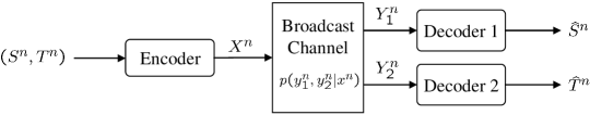
Figure 2: Transmission of correlated sources over a broadcast channel

The problem we are addressing is the simultaneous transmission of two correlated sources $(\mathcal{S},\mathcal{T},p(s,t))$ over a broadcast channel $({\mathcal{X}},{\mathcal{Y}}_{1},{\mathcal{Y}}_{2},p(y_{1},y_{2}|x))$, with one sender and two receivers as shown in Figure 2. Here, the encoder can access both sources $(S,T)$ and the receivers can not communicate with each other. The encoder is given by a mapping $f:\mathcal{S}^{n}\times\mathcal{T}^{n}\rightarrow\mathcal{X}^{n}$. The decoders are given by mappings $g_{1}:\mathcal{Y}_{1}^{n}\rightarrow\mathcal{S}^{n}$ and $g_{2}:\mathcal{Y}_{2}^{n}\rightarrow\mathcal{T}^{n}$. The performance measure associated with this transmission system is the probability of decoding error:

$$Pr[(S^{n},T^{n})\neq(g_{1}(Y_{1}^{n}),g_{2}(Y_{2}^{n}))].$$ (13)

3.1 Basic Concepts

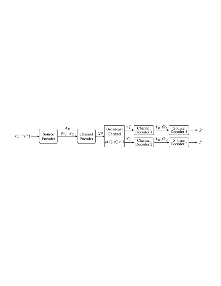
Figure 3: The outputs of sources are first mapped into edges in a bipartite graph, and the edges coming from this graph are reliably transmitted over a broadcast channel

We consider a modular approach to this problem, which is shown in Figure 3. The system has two modules: the source coding module and the channel coding module. The outputs of two correlated sources are first represented efficiently into a triple of messages $(W_{0},W_{1},W_{2})$ in the source coding module. Then, these messages are reliably transmitted over the broadcast channel in the channel coding module. In more detail, the source coding module produces three messages $W_{0},W_{1}$ and $W_{2}$, where $W_{0}$ is a common message to both receivers which contains common information about both sources $S$ and $T$, and $W_{1}$ and $W_{2}$ are private messages which contain the individually remaining information about the source $S$ and $T$ after extracting the common information, respectively. The messages $W_{0},W_{1}$ and $W_{2}$ belong to integer sets $\mathcal{W}_{0}=\{1,2,\ldots,\Delta_{0}\}$, $\mathcal{W}_{1}=\{1,2,\ldots,\Delta_{1}\}$ and $\mathcal{W}_{2}=\{1,2,\ldots,\Delta_{2}\}$, respectively. In general, $W_{0},W_{1}$ and $W_{2}$ are not independent. Then, the channel coding module wants to reliably transmit a message pair $(W_{0},W_{1})$ to receiver 1 and $(W_{0},W_{2})$ to receiver 2.

We assume that there is some kind of correlation between two messages $W_{1}$ and $W_{2}$, i.e., private messages for the receivers can not be chosen independently.

Definition 9

• The private messages of receivers are said to be correlated, if for every $w_{0}\in\mathcal{W}_{0}$, there exists a set $A(w_{0})$ such that $A(w_{0})\subset\mathcal{W}_{1}\times\mathcal{W}_{2}$, and conditioned on $W_{0}=w_{0}$ the message pairs $(W_{1},W_{2})\in A(w_{0})$ are equally likely with probability $\frac{1}{|A(w_{0})|}$, and the message pairs $(W_{1},W_{2})\notin A(w_{0})$ have probability zero.

• The private messages of the receivers are said to be independent, if $A(w_{0})=\mathcal{W}_{1}\times\mathcal{W}_{2}$ for all $w_{0}\in\mathcal{W}_{0}$. In this case, the message pairs $(W_{1},W_{2})$ are equally likely with probability $\frac{1}{|\mathcal{W}_{1}\times\mathcal{W}_{2}|}$.

We use bipartite graphs to model the correlation of the messages, i.e., the set $A(w_{0})$ is taken to be a bipartite graph for all $w_{0}\in\mathcal{W}_{0}$. Let us first define a bipartite graph and related mathematical terms before we discuss the main problem.

Definition 10

• A bipartite graph $G$ is defined as an ordered tuple $G=(A_{1},A_{2},B)$ where $A_{1}$ and $A_{2}$ are two non-empty sets of vertexes, and $B$ is a set of edges where every edge of $B$ joins a vertex in $A_{1}$ to a vertex in $A_{2}$, i.e., $B\subseteq A_{1}\times A_{2}$.

• If $G$ is a bipartite graph, let $V_{1}(G)$ and $V_{2}(G)$ denote the first and the second vertex sets of $G$, respectively, and $E(G)$ denote the edge set of $G$.

• If $(i,j)\in E(G)$, then $i$ and $j$ are said to be adjacent.

• If each vertex in one set is adjacent to every vertex in the other set, then $G$ is said to be a complete bipartite graph. In this case, $E(G)=V_{1}(G)\times V_{2}(G)$.

• The degree of a vertex $v\in V_{i}(G)$ in a graph $G$, denoted by $\mathrm{deg}_{G,i}(v)$, is the number of edges connected to $v$ for $i=1,2$.

• A subgraph of a graph $G$ is a graph whose vertex and edge sets are subsets of those of $G$.

Since we consider a specific type of bipartite graphs in our discussion, let us define those bipartite graphs as well. Although our main results deal with nearly semi-regular graphs, for the purpose of illustration, we consider semi-regular graphs for this section alone.

Definition 11

A bipartite graph $G$ is called semi-regular [34] with parameters $(\theta_{1},\theta_{2},\theta_{1}^{\prime},\theta_{2}^{\prime})$, if it satisfies:

• $|V_{i}(G)|=\theta_{i}$ for $i$=1, 2,

• $\forall u\in V_{1}(G)$, $\mathrm{deg}_{G,1}(u)=\theta_{2}^{\prime}$,

• $\forall v\in V_{2}(G)$, $\mathrm{deg}_{G,2}(v)=\theta_{1}^{\prime}$.

As an example, two semi-regular bipartite graphs with parameters $(4,6,2,3)$ are shown in Figure 4. Note that there exist many semi-regular bipartite graphs with the same set of parameters.

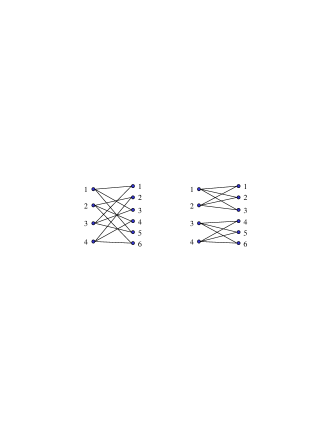
Figure 4: Examples of semi-regular bipartite graphs with parameters $(4,6,2,3)$

Definition 12

A bipartite graph $G$ is called nearly semi-regular with parameters $(\Delta_{1}$, $\Delta_{2}$, $\Delta_{1}^{\prime}$, $\Delta_{2}^{\prime}$, $\mu)$ for $\mu>1$ if it satisfies:

• $|V_{i}(G)|=\Delta_{i}$ for $i=1,2$,

• $\forall u\in V_{1}(G)$, $\Delta_{2}^{\prime}\mu^{-1}\leq\mathrm{deg}_{G,1}(u)\leq\Delta_{2}^{\prime}\mu$,    and   $\forall v\in V_{2}(G)$, $\Delta_{1}^{\prime}\mu^{-1}\leq\mathrm{deg}_{G,2}(v)\leq\Delta_{1}^{\prime}\mu$.

Note that $\mu$ is a slack parameter, which determines the range of degrees of vertexes.

Definition 13

A nearly semi-regular bipartite graph $G$ is said to have parameters $(\Delta_{0},\Delta_{1},\Delta_{2},\Delta_{1}^{\prime},\Delta_{2}^{\prime},\mu)$ for $\mu>1$, if it satisfies the following conditions:

• $G$ is the union of $\Delta_{0}$ disjoint subgraphs $\tilde{G}_{m}$ for $m=1,2,\ldots,\Delta_{0}$ where $\tilde{G}_{m}$ is nearly semi-regular with parameters $(\Delta_{1},\Delta_{2},\Delta_{1}^{\prime},\Delta_{2}^{\prime},\mu)$ as in Definition 12.

• $\forall m\in\{1,2,\ldots,\Delta_{0}\}$, $V_{i}(\tilde{G}_{m})=\{(m-1)\Delta_{i}+1,(m-1)\Delta_{i}+2,\ldots,m\Delta_{i}\}$ for $i$=1, 2,

• $V_{i}(G)=\bigcup_{m=1}^{\Delta_{0}}V_{i}(\tilde{G}_{m})$ for $i$=1, 2,   and    $E(G)=\bigcup_{m=1}^{\Delta_{0}}E(\tilde{G}_{m})$,

A triple of messages (random variables) $(W_{0},W_{1},W_{2})$ can be associated with a graph $G$ with parameters $(\Delta_{0}$, $\Delta_{1}$, $\Delta_{2}$, $\Delta_{1}^{\prime}$, $\Delta_{2}^{\prime}$, $\mu)$ in the following way. $W_{i}\in\mathcal{W}_{i}$ and $\mathcal{W}_{i}=\{1,2,\ldots,\Delta_{i}\}$ for $i=0,1,2$, and an edge $((m-1)\Delta_{1}+i,(m-1)\Delta_{2}+j)\in E(G)$ denotes a realization of the triple of messages $(W_{0},W_{1},W_{2})=(m,i,j)$. In other words, $Pr[(W_{0},W_{1},W_{2})=(m,i,j)]=\frac{1}{|E(G)|}$ if $((m-1)\Delta_{1}+i,(m-1)\Delta_{2}+j)\in E(G)$ and $0$ otherwise. So, different correlation structures of the messages can be modeled by varying the structure of the graph. Figure 5 illustrates an example of a bipartite graph $G$ with parameters $(2,4,4,2,2,1)$ composed of two disjoint subgraphs. This graph can be associated with a triple of messages $(W_{0},W_{1},W_{2})$ where $W_{i}\in\mathcal{W}_{i}$ for $i=1,2,3$ such that $\mathcal{W}_{0}=\{1,2\}$, and $\mathcal{W}_{1}=\mathcal{W}_{2}=\{1,2,3,4\}$. Note that in the figure two subgraphs $\tilde{G}_{1}$ and $\tilde{G}_{2}$ have different edge structures. This implies that the correlation of $(W_{1},W_{2})$ depends on $W_{0}$. $W_{0}$ and $W_{1}$ are independent, and so are $W_{0}$ and $W_{2}$.

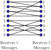
Figure 5: An example of bipartite graph $G$, with parameters $(2,4,4,2,2,1)$, composed of two disjoint subgraphs $\tilde{G}_{1}$ and $\tilde{G}_{2}$ where $\mathcal{W}_{0}=\{1,2\}$, $\mathcal{W}_{1}=\mathcal{W}_{2}=\{1,2,3,4\}$.

3.2 Equivalence classes of graphs

Let us consider the set of all semi-regular bipartite graphs with fixed parameters $(\theta_{1},\theta_{2},\theta_{1}^{\prime},\theta_{2}^{\prime})$. It is well-known that this set can be partitioned into equivalence classes where equivalence relation is permutation and relabeling of the vertexes in the graphs. In more detail, one element (or graph) in a class can be obtained from the other in the same class by permutation and relabeling of the vertexes. However, if two elements (or graphs) belong to different classes, they can not be obtained from each other by permutation and relabeling since they have different correlation structures.

This means that if we have a transmission system which can reliably transmit the edges of a graph $G$ (i.e., the correlation of the message pairs are modeled using $G$) then this transmission system can be used to reliably transmit edges of any graph that belongs to the equivalence class of $G$. Similarly, if one can construct a source representation system that can represent a source pair using a graph $G$ (i.e., the correlation of the index pairs produced by the source encoder is modeled using $G$), then it can be used to represent the source pair using any graph that belongs to the equivalence class of $G$.

4 Broadcast Channels with Correlated Messages

In this section we characterize transmissibility of certain correlated messages over a stationary discrete memoryless broadcast channel.

4.1 Summary of Results

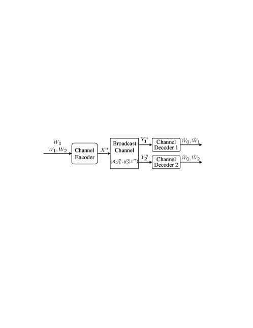
Figure 6: Transmission of correlated messages over the broadcast channel

Although, ideally, we would want to use semi-regular graphs for source representation and communication of information over broadcast channels, for the sake of analytical tractability, as is typical in Shannon theory, we will allow some slack with regard to the degrees of the vertexes of these graphs, and consider the asymptotic case when this slack is bounded in some way.

Definition 14

An $(n,\tau)$-transmission system for a nearly semi-regular bipartite graph $G$ with parameters $(\Delta_{0}$, $\Delta_{1}$, $\Delta_{2}$, $\Delta_{1}^{\prime}$, $\Delta_{2}^{\prime}$, $\mu)$ and a broadcast channel $(\mathcal{X},\mathcal{Y}_{1},\mathcal{Y}_{2},p(y_{1},y_{2}|x))$ is an ordered tuple $(f,g_{1},g_{2})$, consisting of one encoding mapping $f$ and two decoding mappings $g_{1}$ and $g_{2}$ where

• $f:E(G)\rightarrow\mathcal{X}^{n}$, i.e,
  $\forall((m-1)\Delta_{1}+i,(m-1)\Delta_{2}+j)\in E(G)$, assign $x^{n}=f(m,i,j)$ where $m\in\{1,2,\ldots,\Delta_{0}\}$, $i\in\{1,2,\ldots,\Delta_{1}\}$, and $j\in\{1,2,\ldots,\Delta_{2}\}$,

• $g_{i}:\mathcal{Y}_{i}^{n}\rightarrow V_{i}(G)$ for $i=1,2$, i.e., $g_{i}:~{}\mathcal{Y}_{i}^{n}\rightarrow\{1,2,\ldots,\Delta_{0}\}\times\{1,2,\ldots,\Delta_{i}\}$,

• such that a performance measure given by the following average probability of error satisfies:

  $$\tau=\frac{1}{|E(G)|}\sum_{((m-1)\Delta_{1}+i,(m-1)\Delta_{2}+j)\in E(G)}\!\!Pr\left[(g_{1}(Y_{1}^{n}),g_{2}(Y_{2}^{n}))\!\!\neq\!\!((m,i),(m,j))|X^{n}=f(m,i,j)\right].$$ (14)

In Definition 14, the messages $W_{0}$, $W_{1}$ and $W_{2}$ are assumed to have the following distribution:

• Alphabet of $W_{i}$ is $\{1,2,\ldots,\Delta_{i}\}$ for $i=0,1,2$,

• $Pr\{(W_{0},W_{1},W_{2})=(m,i,j)\}=\left\{\begin{array}[]{cl}\frac{1}{E(G)},&\hbox{if $((m-1)\Delta_{1}+i,(m-1)\Delta_{2}+j)\in E(G)$,}\\ 0,&\hbox{else.}\end{array}\right.$

Remark 1

In broadcast channels, the goal of the channel encoder is to reliably transmit two pairs of messages $(W_{0},W_{1})$ and $(W_{0},W_{2})$ to receiver 1 and receiver 2, respectively, over the channel. In terms of graphs, it is to reliably transmit edges of a graph which is associated with the triple of messages $(W_{0},W_{1},W_{2})$ over the channel. As an analogy, the conventional Shannon’s channel coding theorem in a point-to-point communication scenario can be interpreted as finding the maximum number of codewords (colors, if each codeword has a different color) that are distinguishable at the noisy receiver. In the conventional broadcast channel with one sender and two receivers, the goal is to distinguish colors at the noisy receivers, where the first color, which is common to two receivers, can come from one set and the second and the third colors, which are private to each receiver, can come from other two sets, respectively, and all possible combination of triples in the three sets are allowed. A natural question to ask is: if only a fraction of all possible combination of pairs of colors is permitted depending on the common color, what is the maximum size of the sets of these colors which can be reliably distinguished at the receivers.

Definition 15

A tuple of rates $(R_{0},R_{1},R_{2},R_{1}^{\prime},R_{2}^{\prime})$ is said to be achievable for a given broadcast channel with correlated messages, if for all $\epsilon>0$, and for sufficiently large $n$, there exists a bipartite graph $G$ with parameters $(\Delta_{0},\Delta_{1},\Delta_{2},\Delta_{1}^{\prime},\Delta_{2}^{\prime},\mu)$ and an associated $(n,\tau)$-transmission system as defined above satisfying: $\frac{1}{n}\log\Delta_{0}>R_{0}-\epsilon$, $\frac{1}{n}\log\Delta_{i}>R_{i}-\epsilon$, $\frac{1}{n}\log\Delta_{i}^{\prime}>R_{i}^{\prime}-\epsilon$ for $i=1,2$, $\frac{1}{n}\log\mu<\epsilon$ and the corresponding average probability of error $\tau<\epsilon$.

Note that in the above definition, we have taken an optimistic point of view. As long as one can find a sequence of nearly semi-regular graphs where the number of vertexes and the degrees are increasing exponentially with given rates, such that the edges from these graphs are reliably transmitted over the given broadcast channel, we allow the corresponding rate tuple to belong to the achievable rate region. The goal is to find the capacity region $\mathcal{C}_{BC}$ which is the set of all achievable tuple of rates $(R_{0},R_{1},R_{2},R_{1}^{\prime},R_{2}^{\prime})$. In the following we provide an information-theoretic characterization of an achievable rate region. This is an inner bound to the capacity region ${\mathcal{C}_{BC}}$, and is also a per-letter characterization. This is one of the main results of this paper.

Theorem 1

For a discrete memoryless broadcast channel $(\mathcal{X},\mathcal{Y}_{1},\mathcal{Y}_{2},p(y_{1},y_{2}|x))$, $\mathcal{R}_{BC}^{*}\subset\mathcal{C}_{BC}$ where

$$\mathcal{R}_{BC}^{*}=\bigcup_{p(z,u,v,x)}\{(R_{0},R_{1},R_{2},R_{1}^{\prime},R_{2}^{\prime}):~{}~{}~{}$$

$$R_{0} \leq\min\{I(Z;Y_{1}),I(Z;Y_{2})\},$$ (15)

$$R_{1} \leq I(U;Y_{1}|Z),$$ (16)

$$R_{2} \leq I(V;Y_{2}|Z),$$ (17)

$$R_{1}+R_{2}^{\prime}=R_{1}^{\prime}+R_{2} \leq I(U;Y_{1}|Z)+I(V;Y_{2}|Z)-I(U;V|Z)\}$$ (18)

where $Z$, $U$ and $V$ are auxiliary random variables with finite alphabets ${\mathcal{Z}}$, ${\mathcal{U}}$ and ${\mathcal{V}}$, respectively, and $p(z,u,v,x,y_{1},y_{2})=p(z)p(u,v|z)p(x|z,u,v)p(y_{1},y_{2}|x)$ satisfies a Markov chain $(Z,U,V)\rightarrow X\rightarrow(Y_{1},Y_{2})$.

Remark 2

When the private messages are independent, i.e., when all the elements in the set $\mathcal{W}_{1}\times\mathcal{W}_{2}$ can occur with non-zero and equal probability, the rate region becomes exactly the same as Marton’s [12]. However, when the private messages are correlated, i.e., only some elements in the set $\mathcal{W}_{1}\times\mathcal{W}_{2}$ can occur equally likely, the sum rate $R_{1}+R_{2}$ can be larger. As the amount of correlation between the messages increases the achievable rate region also becomes larger.

Remark 3

The limitations of this theorem are as follows. Note that this theorem gives only a partial characterization of the set of all nearly semi-regular graphs whose edges can be reliably transmitted over a broadcast channel. In the formulation of the achievable rate region, we have the freedom of choosing the correlation of the messages for every block-length $n$. The theorem characterizes the rate of exponential growth (as a function of the number of channel uses) of size of certain nearly semi-regular graphs, such that edges coming from any such graph can be reliably transmitted over the broadcast channel. This obviously also means that it is possible to transmit edges of every graph that belongs to the equivalence class of any of these graphs. However, this fact does not mean that the edges of any graph with those parameters can be reliably transmitted.

4.2 Proof of Theorem 1

In this section we prove Theorem 1 by using the method of random coding, random binning, the concept of joint typicality of sequence pairs and some concepts from the theory of random graphs [41]. In addition to using the techniques given in [24], we devise a concept of a “super-bin”, which is a group of consecutive bins, to take into account the correlation between the messages. Given a broadcast channel with distribution $p(y_{1},y_{2}|x)$, consider a fixed joint distribution $p(z,u,v,x)$ = $p(z)$ $p(u,v|z)$ $p(x|z,u,v)$ where $z,u$ and $v$ are auxiliary random variables on $\mathcal{Z}\times\mathcal{U}\times\mathcal{V}$. Also, fix $\epsilon>0$, an integer $n\geq 1$, and positive real numbers $R_{0}$, $R_{1}$, and $R_{2}$.

Random sequences and bin generation: Draw $2^{nR_{0}}$ sequences $Z^{n}(m)$ for $m\in\{1,2,\ldots,2^{nR_{0}}\}$, of length $n$, independently with replacement from $A_{\epsilon}^{(n)}(Z)$ each with probability $\frac{1}{|A_{\epsilon}^{(n)}(Z)|}$ where $A_{\epsilon}^{(n)}(Z)$ is the strongly $\epsilon$-typical set with respect to the distribution $p(z)$ which is a marginal of the joint distribution $p(z,u,v)$ and $|A|$ denotes the cardinality of a set $A$.

For each $m\in\{1,2,\ldots,2^{nR_{0}}\}$, draw $2^{n(I(U;Y_{1}|Z)-\epsilon)}$ $n$-length sequences $U^{n}(k,m)$ for $k\in\{1,2,\ldots,2^{n(I(U;Y_{1}|Z)-\epsilon)}\}$ independently with replacement from $A(U|Z^{n}(m))$ with probability $\frac{1}{|A(U|Z^{n}(m))|}$. Call this collection as ${\bf\Large\mathcal{C}}_{1}(m)$. Here, $A(U|z^{n})$ is the set of $n$-sequences $u^{n}$ which are strongly jointly typical with the sequence $z^{n}$, i.e., for $z^{n}\in A_{\epsilon}^{(n)}(Z)$, the set $A(U|z^{n})\triangleq\{u^{n}|(u^{n},z^{n})\in A_{\epsilon}^{(n)}(U,Z)\}$. Similarly, generate $2^{n(I(V;Y_{2}|Z)-\epsilon)}$ sequences $V^{n}(l,m)$ for $l\in$ $\{1,2,\ldots,$ $2^{n(I(V;Y_{2}|Z)-\epsilon)}\}$ independently with replacement from $A(V|Z^{n}(m))$, where for $z^{n}\in A_{\epsilon}^{(n)}$, the set $A(V|z^{n})\triangleq\{v^{n}|(v^{n},z^{n})\in A_{\epsilon}^{(n)}(V,Z)\}$. Call this collection as ${\bf\Large\mathcal{C}}_{2}(m)$. Without loss of generality $2^{n(I(U;Y_{1}|Z)-\epsilon)}$ and $2^{n(I(V;Y_{2}|Z)-\epsilon)}$ are assumed to be integers.

Next, for each $m$ in $\{1,2,\ldots,2^{nR_{0}}\}$, define random bins $B(i,m)$ and $C(j,m)$ for $i\in\{1,2,\ldots,2^{nR_{1}}\}$ and $j\in\{1,2,\ldots,2^{nR_{2}}\}$ such that

$$B(i,m) =\{U^{n}(k,m)~{}|~{}k\in[(i-1)\cdot 2^{n(I(U;Y_{1}|Z)-R_{1}-\epsilon)}+1,~{}i\cdot 2^{n(I(U;Y_{1}|Z)-R_{1}-\epsilon)}]\}$$ (19)

$$C(j,m) =\{V^{n}(l,m)~{}|~{}l\in[(j-1)\cdot 2^{n(I(V;Y_{2}|Z)-R_{2}-\epsilon)}+1,~{}j\cdot 2^{n(I(V;Y_{2}|Z)-R_{2}-\epsilon)}]\}$$ (20)

where without loss of generality $2^{n(I(U;Y_{1}|Z)-R_{1}-\epsilon)}$ and $2^{n(I(V;Y_{2}|Z)-R_{2}-\epsilon)}$ are considered to be integers, and $[a,b]$ denotes the set of integers from $a$ to $b$. This imposes the following constraints on $R_{1}$ and $R_{2}$: $R_{1}\leq I(U;Y_{1}|Z)-\epsilon$, and $R_{2}\leq I(V;Y_{2}|Z)-\epsilon$.

Figure 7: A subgraph $\tilde{\mathbb{G}}_{1}$ ($m=1$) with parameters $(2^{nR_{1}},2^{nR_{2}},2^{nR_{1}^{\prime}},2^{nR_{2}^{\prime}},\mu)$.

Graph generation: As shown in Figure 7, for each $m$ in $\{1,2,\ldots,2^{nR_{0}}\}$, a random graph $\tilde{\mathbb{G}}_{m}$ can be associated with the bins as follows. (1) $V_{1}(\tilde{\mathbb{G}}_{m})=\{(m-1)2^{nR_{1}}+1,\ldots,m2^{nR_{1}}\}$ and $V_{2}(\tilde{\mathbb{G}}_{m})=\{(m-1)2^{nR_{2}}+1,\ldots,m2^{nR_{2}}\}$, (2) $\forall(i,j)\in V_{1}(\tilde{\mathbb{G}}_{m})\times V_{2}(\tilde{\mathbb{G}}_{m})$, $(i,j)\in E(\tilde{\mathbb{G}}_{m})$ if and only if there exists in $B(i,m)\times C(j,m)$ at least one $\epsilon$-strongly jointly typical sequence pair that belongs to $A(U,V|Z^{n}(m))$, where $A(U,V|z^{n})$ is the set of pairs of sequences that are jointly $\epsilon$-typical with the sequence $z^{n}$, i.e., for $z^{n}\in A_{\epsilon}^{(n)}(Z)$, the set $A(U,V|z^{n})$$\triangleq\{(u^{n},v^{n})|(u^{n},v^{n},z^{n})\in A_{\epsilon}^{(n)}(U,V,Z)\}$. Let $\mathbb{G}$ denote the random graph that is the union of $2^{nR_{0}}$ random graphs $\tilde{\mathbb{G}}_{m}$ for $m\in\{1,2,\ldots,2^{nR_{0}}\}$.

Codebook generation: A random channel codebook $\mathbb{C}$ can be generated from the graph $\mathbb{G}$ as follows. For every $m\in\{1,2,\ldots,2^{nR_{0}}\}$, and every $(i,j)\in E(\tilde{\mathbb{G}}_{m})$, first find one pair of sequences $(U^{n}(k,m),V^{n}(l,m))\in A(U,V|Z^{n}(m))\cap(B(i,m)\times C(j,m))$. Then draw a random codeword $X^{n}(m,i,j)=f(m,i,j)$ uniformly from $A(X|U^{n}(k),V^{n}(l),Z^{n}(m))$, where $A(X|u^{n},v^{n},z^{n})\triangleq\{x^{n}|(x^{n},u^{n},v^{n},z^{n})\in A_{\epsilon}^{(n)}(X,U,V,Z)\}$. Thus the size of the codebook is equal to the size of the edge set of the graph $\mathbb{G}$, i.e., $|\mathbb{C}|=|E(\mathbb{G})|$.

Encoding error events due to the degree condition: Before we proceed to the encoding and decoding procedure, we need to make sure that the generated codebooks satisfy certain properties. If vertexes of the graph $\mathbb{G}$ do not satisfy the degree conditions, the message pairs can not be transmitted with arbitrarily small probability of error. Let

$$A=I(U;Y_{1}|Z)+I(V;Y_{2}|Z)-I(U;V|Z)-2\epsilon,$$ (21)

and choose $R^{\prime}_{1}=A-R_{2}$ and $R^{\prime}_{2}=A-R_{1}$. Since $0\leq R^{\prime}_{i}\leq R_{i}$ for $i=1,2$, we have the following conditions on $R_{1}$ and $R_{2}$:

$$\max\{R_{1},R_{2}\}\leq A\leq R_{1}+R_{2}.$$ (22)

In summary, the nonnegative tuple $(R_{1},R_{2},R^{\prime}_{1},R^{\prime}_{2})$ that we use for the random coding satisfies:

$$R_{1}\leq I(U;Y_{1}|Z)-\epsilon,\ \ \ R_{1}\leq I(V;Y_{2}|Z)-\epsilon,$$ (23)

$$R_{1}+R^{\prime}_{2}=R_{2}+R^{\prime}_{1}=I(U;Y_{1}|Z)+I(V;Y_{2}|Z)-I(U;V|Z)-2\epsilon.$$ (24)

For a precise characterization of the error events, we need a function of $\epsilon$, and in turn certain properties of typical sets. For any triple $(U,V,Z)$ of finite-valued random variables, there exists [35] a continuous positive function $\epsilon_{1}(\epsilon)$ (that depends on the triple) such that (a) $\epsilon_{1}(\epsilon)\rightarrow 0$ as $\epsilon\rightarrow 0$ and (b) for all $\epsilon>0$ (sufficiently small), there exists an integer $N_{0}(\epsilon)>0$ such that $\forall n>N_{0}(\epsilon)$ the following conditions hold simultaneously

• for all $z^{n}\in A_{\epsilon}^{(n)}(Z)$,

  $$2^{n(H(U|Z)-\epsilon_{1})}\leq|A(U|z^{n})|\leq 2^{n(H(U|Z)+\epsilon_{1})}$$ (25)

  $$2^{n(H(V|Z)-\epsilon_{1})}\leq|A(V|z^{n})|\leq 2^{n(H(V|Z)+\epsilon_{1})}$$ (26)

  $$2^{n(H(U,V|Z)-\epsilon_{1})}\leq|A(U,V|z^{n})|\leq 2^{n(H(U,V|Z)+\epsilon_{1})}$$ (27)

• $\forall(u^{n},z^{n})\in A_{\epsilon}^{(n)}(U,Z)$

  $$2^{n(H(V|U,Z)-\epsilon_{1})}\leq|A(V|u^{n},z^{n})|\leq 2^{n(H(V|U,Z)+\epsilon_{1})}$$ (28)

• $\forall(v^{n},z^{n})\in A_{\epsilon}^{(n)}(V,Z)$

  $$2^{n(H(U|V,Z)-\epsilon_{1})}\leq|A(U|v^{n},z^{n})|\leq 2^{n(H(U|V,Z)+\epsilon_{1})}.$$ (29)

Coming back to the encoding error event, an error will be declared if either one of the following events occur. Let $\epsilon^{\prime}>3\epsilon_{1}>0$.

• $E_{1}$: $\exists i\in V_{1}(\mathbb{G})$ such that $\left|\frac{1}{n}\log{\rm deg}_{\mathbb{G},1}(i)-R_{2}^{\prime}\right|>\epsilon^{\prime}$,

• $E_{2}$: $\exists j\in V_{2}(\mathbb{G})$ such that $\left|\frac{1}{n}\log{\rm deg}_{\mathbb{G},2}(j)-R_{1}^{\prime}\right|>\epsilon^{\prime}$.

Now we show that the probability of these error events can be made arbitrarily small under certain conditions. Let us define four events as follows.

• $E_{0,1}$ : $\exists i\in V_{1}(\mathbb{G})$ such that ${\rm deg}_{\mathbb{G},1}(i)<2^{n(R^{\prime}_{2}-\epsilon^{\prime})}$

• $E_{0,2}$ : $\exists j\in V_{2}(\mathbb{G})$ such that ${\rm deg}_{\mathbb{G},2}(j)<2^{n(R^{\prime}_{1}-\epsilon^{\prime})}$

• $E^{*}_{0,1}$ : $\exists i\in V_{1}(\mathbb{G})$ such that ${\rm deg}_{\mathbb{G},1}(i)>2^{n(R^{\prime}_{2}+\epsilon^{\prime})}$

• $E^{*}_{0,2}$ : $\exists j\in V_{2}(\mathbb{G})$ such that ${\rm deg}_{\mathbb{G},2}(j)>2^{n(R^{\prime}_{1}+\epsilon^{\prime})}$

Toward proving the required statements, we need a lemma given in [42] about certain properties of typical sets.

Lemma 1

For any triple of finite-valued random variables $(U,V,Z)$, any $\epsilon>0$ (sufficiently small), any two positive real numbers $R_{1}$ and $R_{2}$ such that $R_{1}+R_{2}>I(U;V|Z)$, and any $z^{n}\in A_{\epsilon}^{(n)}(Z)$ consider the following random experiment. Generate two collections of sequences ${\bf\Large\mathcal{C}}_{U}(z^{n})$ and ${\bf\Large\mathcal{C}}_{V}(z^{n})$ of size $2^{nR_{1}}$ and $2^{nR_{2}}$ from $A(U|z^{n})$ and $A(V|z^{n})$, respectively, with uniform distribution and with replacement. Let $P_{\epsilon}(z^{n},R_{1},R_{2})$ denote the probability that $|({\bf\Large\mathcal{C}}_{U}\times{\bf\Large\mathcal{C}}_{V})\cap A(U,V|z^{n})|=0$. Then $\forall\epsilon>0$, $\forall R_{1},R_{2}$ with $R_{1}+R_{2}>I(U;V|Z)$ and $\forall z^{n}\in A_{\epsilon}^{(n)}(Z)$,

$$\lim_{n\rightarrow\infty}-\frac{1}{n}\log P_{\epsilon}(z^{n},R_{1},R_{2})=\infty.$$ (30)

Proof: See Theorem 2.1 of [42].

The proofs of the next two lemmas use this result.

Lemma 2

For any $\epsilon>0$, and sufficiently large $n$:

$$P\{E_{0,i}\}<\frac{\epsilon}{12},~{}~{}\mbox{for $i=1,2$}$$ (31)

Proof: Refer to Appendix A.

Lemma 3

For any $\epsilon>0$, and sufficiently large $n$:

$$P\{E_{0,i}^{*}\}<\frac{\epsilon}{12},~{}~{}\mbox{for $i=1,2$}$$ (32)

Proof: Refer to Appendix B.

Note that $E_{1}=E_{0,1}\cup E_{0,1}^{*}$ and $E_{2}=E_{0,2}\cup E_{0,2}^{*}$. Thus, according to the Lemma 2 and 3, it is easy to see that, for sufficiently large $n$, $P(E_{1})<\frac{\epsilon}{6}$, and $P(E_{2})<\frac{\epsilon}{6}$, if $R_{2}^{\prime}=I(U;Y_{1}|Z)-R_{1}+I(V;Y_{2}|Z)-I(U;V|Z)-2\epsilon$ and $R_{1}^{\prime}=I(U;Y_{1}|Z)-R_{2}+I(V;Y_{2}|Z)-I(U;V|Z)-2\epsilon$, respectively. So, it is shown that with high probability we can obtain a nearly semi-regular bipartite graph $\mathbb{G}$ composed of $2^{nR_{0}}$ disjoint subgraphs $\tilde{\mathbb{G}}_{m}$ such that for each $m$, each vertex in $V_{1}(\tilde{\mathbb{G}}_{m})$ has degree nearly equal to $2^{nR^{\prime}_{2}}$ and each vertex in $V_{2}(\tilde{\mathbb{G}}_{m})$ has degree nearly equal to $2^{nR^{\prime}_{1}}$. The size of $V_{1}(\tilde{\mathbb{G}}_{m})$ is $2^{nR_{1}}$ and that of $V_{2}(\tilde{\mathbb{G}}_{m})$ is $2^{nR_{2}}$.

Choosing message correlation: If none of the above two error events $E_{1}$ and $E_{2}$ occurs, choose $G=\mathbb{G}$. Clearly $G$ has parameters $(2^{nR_{0}}$, $2^{nR_{1}}$, $2^{nR_{2}}$, $2^{nR_{1}^{\prime}}$, $2^{nR_{2}^{\prime}}$, $2^{n\epsilon^{\prime}})$. If any of the above two error events occurs, then pick any graph with parameters $(2^{nR_{0}}$, $2^{nR_{1}}$, $2^{nR_{2}}$, $2^{nR_{1}^{\prime}}$, $2^{nR_{2}^{\prime}}$, $2^{n\epsilon^{\prime}})$ and call it as $G$. The distribution of $W_{0}$, $W_{1}$ and $W_{2}$ is chosen as follows. $Pr\{(W_{0},W_{1},W_{2})=(m,i,j)\}=\frac{1}{E(G)}$ if $((m-1)2^{nR_{1}}+i,(m-1)2^{nR_{2}}+j)\in E(G)$ and $Pr\{(W_{0},W_{1},W_{2})=(m,i,j)\}=0$ else. For this graph $G$, and the given broadcast channel, using the above random codebook $\mathbb{C}$, we construct an $(n,\tau)$-transmission system, where $\tau$ will be specified in the sequel.

Encoding: Sender transmits the codeword $X^{n}(m,i,j)$ over the channel to deliver two pair of messages $(m,i)$ and $(m,j)$ to receiver 1 and receiver 2, respectively.

Decoding: Both Receiver 1 and Receiver 2 first find the unique index $\hat{m}$ such that $Z^{n}(\hat{m})$ is jointly typical with received sequence $Y_{1}^{n}$ and $Y_{2}^{n}$, respectively. Then, Receiver 1 finds the unique index $\hat{k}$ such that $U^{n}(\hat{k},\hat{m})$ is jointly typical with the received sequence $Y_{1}^{n}$ and $Z^{n}(\hat{m})$, i.e., $(U^{n}(\hat{k},\hat{m}),Y_{1}^{n},Z^{n}(\hat{m}))\in A_{\epsilon}^{(n)}(U,Y_{1},Z)$. Similarly, Receiver 2 finds the unique index $\hat{l}$ such that $(V^{n}(\hat{l},\hat{m}),Y_{2}^{n},Z^{n}(\hat{m}))\in A_{\epsilon}^{(n)}(V,Y_{2},Z)$. Then, each receiver finds the decoded private messages $\hat{i}$ and $\hat{j}$ such that $U^{n}(\hat{k},\hat{m})\in B(\hat{i},\hat{m})$ and $V^{n}(\hat{l},\hat{m})\in C(\hat{j},\hat{m})$, respectively. Otherwise, an error will be declared.

Probability of error analysis: So, the probability of error $P(E)$ can be given by

$$P(E) =P(E_{1}\cup E_{2})P(E|E_{1}\cup E_{2})+P(E\cap E_{1}^{c}\cap E_{2}^{c})$$ (33)

$$\leq P(E_{1}\cup E_{2})+P(E\cap E_{1}^{c}\cap E_{2}^{c})$$ (34)

The second probability in the above equation can be bounded as given in the following lemma.

Lemma 4

For any $\epsilon>0$, and sufficiently large $n$,

$$P(E\cap E_{1}^{c}\cap E_{2}^{c})<\frac{2\epsilon}{3}$$ (35)

provided

$$R_{0} \leq\min\{I(Z;Y_{1}),I(Z;Y_{2})\}-\epsilon.$$ (36)

Proof: Refer to Appendix C.
Therefore, by applying the union bound we have $P(E)\leq P(E_{1})+P(E_{2})+P(E\cap E_{1}^{c}\cap E_{2}^{c})\leq\epsilon$.

Since in every realization of random codebooks, we have chosen a nearly semi-regular graph $G$ with parameters $(2^{nR_{0}}$, $2^{nR_{1}}$, $2^{nR_{2}}$, $2^{nR_{1}^{\prime}}$, $2^{nR_{2}^{\prime}}$, $2^{n\epsilon^{\prime}})$, and averaged over the ensemble of random codebooks, the average probability of error is smaller than $\epsilon$, there must exist a graph $G$ with parameters $(2^{nR_{0}}$, $2^{nR_{1}}$, $2^{nR_{2}}$, $2^{nR_{1}^{\prime}}$, $2^{nR_{2}^{\prime}}$, $2^{n\epsilon^{\prime}})$ and a codebook such that the average probability of error is smaller than $\epsilon$. This is true only under the condition given by the statement of the theorem. Hence, the proof of Theorem 1 has been completed. $\blacksquare$

4.3 The Capacity Region of a Broadcast Channel with One Deterministic Component with Correlated Messages

In this section, we consider the capacity region of broadcast channels with one deterministic component with correlated messages, $\mathcal{\tilde{C}}_{BC}$, when there is no common message, i.e., when $R_{0}=0$. In this case, as expected, we can provide a converse coding theorem.

Theorem 2

For a discrete memoryless semi-deterministic broadcast channel where $y_{1}=f_{1}(x)$ and the probability of $y_{2}$ given $x$ is $p(y_{2}|x)$, $\mathcal{\tilde{R}}_{BC}^{*}=\mathcal{\tilde{C}}_{BC}$ where

$$\mathcal{\tilde{R}}_{BC}^{*}=\bigcup_{p(v,x)}\{(R_{1},R_{2},R_{1}^{\prime},R_{2}^{\prime}):~{}~{}~{}~{}~{}$$

$$R_{1} \leq H(Y_{1})$$ (38)

$$R_{2} \leq I(V;Y_{2})$$ (39)

$$R_{1}+R_{2}^{\prime}=R_{1}^{\prime}+R_{2} \leq H(Y_{1}|V)+I(V;Y_{2})\}$$ (40)

for some $p(v,x)$ on ${\mathcal{V}}\times{\mathcal{X}}$, where $V$ is an auxiliary random variable with finite alphabet ${\mathcal{V}}$ such that $V\rightarrow X\rightarrow(Y_{1},Y_{2})$, $|{\mathcal{V}}|\leq|{\mathcal{X}}|+2$.

Proof: See Appendix D.

5 Representation of Correlated Sources into Graphs

In this section, we consider the problem of representation of correlated sources into graphs for transmission over broadcast channels, i.e., source coding module in broadcast channels with correlated sources. This problem can be interpreted as Gray-Wyner problem with correlated messages. In in this setup, the source encoder can access both sources to be transmitted, but the source decoders can not collaborate with each other. We consider two correlated sources $(\mathcal{S},\mathcal{T},p(s,t))$.

5.1 Summary of Results

In this problem, the goal is to reliably represent two correlated sources into a triple of messages $(W_{0},W_{1},W_{2})$ which can be associated with a nearly semi-regular bipartite graph $G$ with parameters $(\Delta_{0},\Delta_{1},\Delta_{2},\Delta_{1}^{\prime},\Delta_{2}^{\prime},\mu)$ as defined in Definition 13. As shown in Figure 8, the output of source encoder is the triple $W_{0}$, $W_{1}$ and $W_{2}$. We assume that two pairs of messages $(W_{0},W_{1})$ and $(W_{0},W_{2})$ are sent to receiver 1 and receiver 2, respectively, over the channel without error. From the received message pairs, the two source decoders wish to reliably reconstruct the original source sequences $S^{n}$ and $T^{n}$, respectively, without communicating with each other. For ease of exposition let is consider two simple functions $I_{1}$ and $I_{2}$ both having domain as $\mathbb{Z}\times\mathbb{Z}$ and range as $\mathbb{Z}$ given by $I_{1}(a,b)=a$ and $I_{2}(a,b)=b$ for all $(a,b)\in\mathbb{Z}\times\mathbb{Z}$.

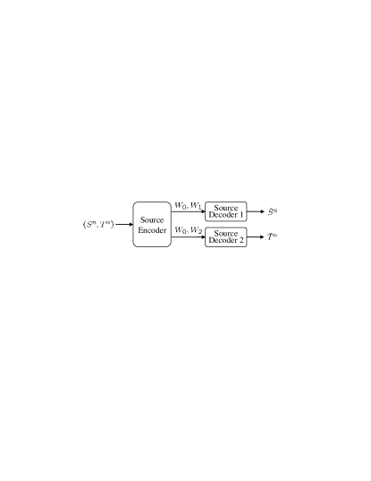
Figure 8: Gray-Wyner problem with correlated messages

Definition 16

An $(n,\tau)$-transmission system for a nearly semi-regular bipartite graph $G$ with parameters $(\Delta_{0}$, $\Delta_{1}$, $\Delta_{2}$, $\Delta_{1}^{\prime}$, $\Delta_{2}^{\prime}$, $\mu)$ and a pair of correlated sources $({\mathcal{S}},{\mathcal{T}},p(s,t))$ is an ordered tuple $(f,g_{1},g_{2})$, consisting of one encoding mapping $f$ and two decoding mappings $g_{1}$ and $g_{2}$ where

• $f:\mathcal{S}^{n}\times\mathcal{T}^{n}\rightarrow E(G)$,

• $g_{1}:V_{1}(G)\rightarrow\mathcal{S}^{n}$, $g_{2}:V_{2}(G)\rightarrow\mathcal{T}^{n}$,

• such that a performance measure given by the probability of error satisfies:

  $$\tau =Pr\{(g_{1}(I_{1}(f(S^{n},T^{n}))),g_{2}(I_{2}(f(S^{n},T^{n}))))\!\neq\!(S^{n},T^{n})\}.$$ (41)

Now we define achievable rates for this problem as follows.

Definition 17

A tuple of rates $(R_{0},R_{1},R_{2},R_{1}^{\prime},R_{2}^{\prime})$ is said to be achievable for a pair of correlated sources $(\mathcal{S},\mathcal{T},p(s,t))$ (for transmission over broadcast channels), if for all $\epsilon>0$, and for all sufficiently large $n$, there exists a bipartite graph $G$ with parameters $(\Delta_{0},\Delta_{1},\Delta_{2},\Delta_{1}^{\prime},\Delta_{2}^{\prime},\mu)$ and an associated $(n,\tau)$-transmission system as defined above satisfying: $\frac{1}{n}\log\Delta_{i}<R_{i}+\epsilon$ for $i=0,1,2$, $\frac{1}{n}\log\Delta_{j}^{\prime}<R_{j}^{\prime}+\epsilon$ for $j=1,2$, $\frac{1}{n}\log\mu<\epsilon$ and the corresponding probability of error $\tau<\epsilon$.

The goal is to find the achievable rate region $\mathcal{R}_{GW}$ which is the set of all achievable tuple of rates $(R_{0},R_{1},R_{2},R_{1}^{\prime},R_{2}^{\prime})$. We have obtained an inner bound to the achievable rate region. It is one of the main results of this paper and is given by the following theorem.

Theorem 3

$\mathcal{R}_{GW}^{*}\subset\mathcal{R}_{GW}$ where

$$\mathcal{R}_{GW}^{*}=\bigcup_{p(z|s,t)}\{(R_{0},R_{1},R_{2},R_{1}^{\prime},R_{2}^{\prime}) :$$

$$R_{0} \geq I(S,T;Z),$$ (42)

$$R_{1} \geq H(S|Z),\ \ \ R_{2}\geq H(T|Z),$$ (43)

$$R_{1}^{\prime} \geq H(S|T,Z),\ \ \ R_{2}^{\prime}\geq H(T|S,Z),$$ (44)

where $Z$ is an auxiliary random variable with a finite alphabet $\mathcal{Z}$ such that $p(z,s,t)=p(s,t)p(z|s,t)$.

Remark 4

Note that we can obtain $R_{0}+R_{1}+R_{2}^{\prime}=R_{0}+R_{1}^{\prime}+R_{2}\geq H(S,T)$ by combining the conditions in Theorem 3. This means that in every nearly semi-regular bipartite graph used to represent the source, as expected, the total number of edges must be greater than or equal to $2^{nH(S,T)}$.

5.2 Proof of Theorem 3

In this section, we present a proof of Theorem 3. We use a random coding procedure and the notion of strongly jointly typical sequences. Let us consider a fixed finite set ${\mathcal{Z}}$, and a joint probability distribution $p(z,s,t)$ on $\mathcal{Z}\times\mathcal{S}\times\mathcal{T}$. Also fix $\epsilon>0$, and real numbers $R_{0}$, $R_{1}$, $R_{2}$, $R^{\prime}_{i}=R_{i}-I(S;T|Z)$ for $i=1,2$. Without loss of generality we assume that $R_{i}>I(S;T|Z)$ for $i=1,2$.

Random sequence generation: First, draw $2^{nR_{0}}$ sequences $Z^{n}(m)$, $m\in\{1,2$, $\ldots,2^{nR_{0}}\}$, of length $n$, independently from the strongly $\epsilon$-typical set $A_{\epsilon}^{(n)}(Z)$. That is, $P\{Z_{m}^{n}=z^{n}\}=\frac{1}{|A_{\epsilon}^{(n)}(Z)|}$ if $z^{n}\in A_{\epsilon}^{(n)}(Z)$, and $P\{Z_{m}^{n}=z^{n}\}=0$ if $z^{n}\notin A_{\epsilon}^{(n)}(Z)$. For every $m\in\{1,2,\ldots,2^{nR_{0}}\}$, draw $2^{nR_{1}}$ sequence from $A_{\epsilon}^{(n)}(S|Z^{n}(m))$ independently, equally likely and with replacement. Call this collection $B(m)$. Denote the $i$th sequence as $S^{n}(i,m)$. By collecting these $2^{nR_{0}}$ bins the first codebook $\mathbb{C}_{1}$ can be obtained. In other words, $\mathbb{C}_{1}=\{B(1),B(2),\ldots,B(2^{nR_{0}})\}$.

Similarly, for every $m\in\{1,2,\ldots,2^{nR_{0}}\}$, construct a bin $C(m)$ containing $2^{nR_{2}}$ sequences from $A_{\epsilon}^{(n)}(T|Z^{n}(m))$. Let the $j$th sequence in $C(m)$ be denoted by $T^{n}(j,m)$. The second codebook $\mathbb{C}_{2}$ can be similarly generated, i.e., $\mathbb{C}_{2}=\{C(1),C(2),\ldots,C(2^{nR_{0}})\}$.

Graph generation: Now we generate a bipartite graph $\mathbb{G}$ from the codebooks $\mathbb{C}_{1}$ and $\mathbb{C}_{2}$ as follows:

• $\mathbb{G}$ is composed of $2^{nR_{0}}$ disjoint subgraphs $\tilde{\mathbb{G}}_{m}$ for $m\in\{1,2,\ldots,2^{nR_{0}}\}$,

• $V_{i}(\mathbb{G})\!=\!\cup_{m=1}^{2^{nR_{0}}}V_{i}(\tilde{\mathbb{G}}_{m})$ for $i=1,2$,    $E(\mathbb{G})=\cup_{m=1}^{2^{nR_{0}}}E(\tilde{\mathbb{G}}_{m})$,

• $\forall m\!\in\!\{1,2,\ldots,2^{nR_{0}}\}$, $V_{1}(\tilde{\mathbb{G}}_{m})\!=\!\{(m-1)2^{nR_{1}}-1,\ldots,m2^{nR_{1}}\}$, $V_{2}(\tilde{\mathbb{G}}_{m})$=$\{(m-1)2^{nR_{2}}-1,\ldots,m2^{nR_{2}}\}$,

• $\forall m\!\in\!\{1,2,\ldots,2^{nR_{0}}\}$, $(i,j)\in E(\tilde{\mathbb{G}}_{m})$ if and only if $(S^{n}(i,m)$, $T^{n}(j,m)$, $Z^{n}(m))$ $\in A_{\epsilon}^{(n)}(S,T,Z)$.

Encoding error events: Before we proceed further, let us make sure that the generated codebooks satisfy certain properties. If the vertexes of $\mathbb{G}$ do not satisfy certain degree requirements, we may not be able to reliably represent the sources using this graph. For the triple $(S,T,Z)$, consider the function $\epsilon_{1}(\epsilon)$ as defined in (25)-(29). Let $\epsilon^{\prime}>3\epsilon_{1}>0$. An encoding error will be declared if either one of the following events occurs.
$E_{1}:\exists i\in V_{1}(\mathbb{G})\mbox{ such }\mbox{ that }|\frac{1}{n}\log{\rm deg}_{\mathbb{G},1}-R^{\prime}_{2}|>\epsilon^{\prime}$,
$E_{2}:\exists j\in V_{2}(\mathbb{G})\mbox{ such }\mbox{ that }|\frac{1}{n}\log{\rm deg}_{\mathbb{G},2}-R^{\prime}_{1}|>\epsilon^{\prime}$.

Using the following lemma it can be shown that the probability of these two events can be made arbitrarily small for large $n$.

Lemma 5

For any $\epsilon>0$, and sufficiently large $n$, we have $P(E_{i})<\frac{\epsilon}{8},\ \ {\rm for}\ \ i=1,2.$

Proof: The proofs of these two results are similar, respectively, to those of Lemma 2 and Lemma 3. Hence for conciseness we omit the proof.

So by Lemma 5, $P(E_{1})+P(E_{2})<\frac{\epsilon}{4}$. Hence we can obtain a bipartite graph $\mathbb{G}$ where each vertex in $V_{1}(\mathbb{G})$ has degree nearly equal to $2^{nR^{\prime}_{2}}$ and each vertex in $V_{2}(\mathbb{G})$ has degree nearly equal to $2^{nR^{\prime}_{1}}$.

Choosing message correlation: If none of the above error events $E_{1}$ and $E_{2}$ occurs, then choose $G=\mathbb{G}$. If any of the above two error events occurs, then pick any graph with parameters $(2^{nR_{0}},2^{nR_{1}},2^{nR_{2}},2^{nR^{\prime}_{1}},2^{nR^{\prime}_{2}},2^{n\epsilon^{\prime}})$ and call it as $G$ and no guarantee will be given regarding the probability of decoding error. For this graph $G$, and the given correlated sources $S$ and $T$, using the above random codebooks $\mathbb{C}_{1}$ and $\mathbb{C}_{2}$, we construct an $(n,\tau)$-transmission system, where $\tau$ will be specified in the sequel.

Encoding: If $(E_{1}\cup E_{2})$ occurs, then the encoder is some arbitrary mapping $\mathcal{S}^{n}\times\mathcal{T}^{n}\rightarrow E(G)$. Otherwise, for a given $(S^{n},T^{n})\!\in\!A_{\epsilon}^{(n)}(S,T)$, find an index $m$, for $m\in\{1,2,$ $\ldots,2^{nR_{0}}\}$, such that $(S^{n}$, $T^{n}$, $Z^{n}(m))$ $\in A_{\epsilon}^{(n)}(S,T,Z)$. If there is no such index $m$, let $m$ be a random index chosen uniformly from $\{1,2,\ldots,2^{nR_{0}}\}$. Also, find a pair of indexes $(i,j)$ where $i$ (and $j$, respectively) is the index such that $S^{n}(i,m)=S^{n}$ (and $T^{n}(j,m)=T^{n}$, respectively). If there is no such sequence pair let $(i,j)$ be a random edge from the corresponding sub-graph of $G$. The encoder sends $(m,i)$ and $(m,j)$ to receiver 1 and receiver 2, respectively.

Decoding: Given the received index pair $(m,i)$, receiver 1 declares $\hat{S}^{n}=S^{n}(i,m)$. Similarly, given $(m,j)$, receiver 2 declares $\hat{T}^{n}=T^{n}(j,m)$.

Probability of error analysis: Let $E$ denote the event $\{(g_{1}(m,i),g_{2}(m,j))\!\neq\!(S^{n},T^{n})\}$, that the reconstruction vector pair is not equal to the source vector pair. The probability of error $P(E)$ can be given by

$$P(E) =P(E_{1}\!\cup\!E_{2})P(E|E_{1}\!\cup\!E_{2})\!+\!P(E\cap E_{1}^{c}\cap E_{2}^{c})$$ (45)

$$\leq P(E_{1}\!\cup\!E_{2})+P(E\cap E_{1}^{c}\cap E_{2}^{c}).$$ (46)

The second probability in the above equation can be bounded as given in the following lemma.

Lemma 6

For any $\epsilon>0$, and sufficiently large $n$,

$$P(E\cap E_{1}^{c}\cap E_{2}^{c})<\frac{3\epsilon}{4}$$ (47)

provided

$$R_{0}>I(S,T;Z)+\epsilon_{2}(\epsilon),\ \ R_{1}>H(S|Z)+\epsilon_{1}(\epsilon),\ \ R_{2}>H(T|Z)+\epsilon_{1}(\epsilon),$$ (48)

where $\epsilon_{2}(\epsilon)\rightarrow 0$ as $\epsilon\rightarrow 0$ and $\epsilon_{2}(\epsilon)>0$.

Proof: Refer to Appendix E.

Thus, $P(E)\leq P(E_{1})\!+\!P(E_{2})\!+\!P(E\cap E_{1}^{c}\cap E_{2}^{c})<\epsilon$. Therefore $P(E)<\epsilon$ for sufficiently large $n$ and under the conditions given by the theorem. In every realization of random codebooks we have obtained a graph $G$ with the same set of parameters, and averaged over this ensemble, we have made sure that the probability of error is within the tolerance level of $\epsilon$. Hence, the proof of the direct coding theorem is completed. $\blacksquare$

5.3 Outer bound

In this section we provide a partial converse for Theorem 3.

Theorem 4

$\mathcal{R}_{GW}\subset\mathcal{R}_{GW}^{**}$ where

$$\mathcal{R}_{GW}^{**}=\bigcup_{p(w|s,t)}\{(R_{0},R_{1},R_{2},R_{1}^{\prime},R_{2}^{\prime}) :$$

$$R_{0} \geq I(S,T;Z),$$ (49)

$$R_{1} \geq H(S|Z),\ \ \ R_{2}\geq H(T|Z),$$ (50)

$$R_{1}+R_{2}^{\prime} =R_{1}^{\prime}+R_{2}\geq H(S,T|Z)\},$$ (51)

where $Z$ is an auxiliary random variable such that $p(z,s,t)=p(s,t)p(z|s,t)$.

Proof: Refer to Appendix F.

5.4 An interpretation of the rate region

We have shown that for sufficiently large block length $n$, a pair correlated sources $(S,T)$ can be represented into a nearly semi-regular graph $G$ with parameters $(2^{nR_{0}}$, $2^{nR_{1}}$, $2^{nR_{2}}$, $2^{nR_{1}^{\prime}}$, $2^{nR_{2}^{\prime}}$, $2^{n\epsilon^{\prime}}$) as shown in Figure 9.

Figure 9: Graph $G$ with parameters $(2^{nR_{0}}$, $2^{nR_{1}}$, $2^{nR_{2}}$, $2^{nR_{1}^{\prime}}$, $2^{nR_{2}^{\prime}}$, $2^{n\epsilon^{\prime}})$ composed of $2^{nR_{0}}$ subgraphs $\tilde{G}_{m}$ with parameters ($2^{nR_{1}}$, $2^{nR_{2}}$, $2^{nR_{1}^{\prime}}$, $2^{nR_{2}^{\prime}}$, $2^{n\epsilon^{\prime}}$)

Note that many different graphs can be used to represent a pair correlated sources without increasing the amount of “global” redundancy, i.e., the sum rate satisfies: $R_{0}+R_{1}+R_{2}^{\prime}=H(S,T)$. This can be seen from the fact that the total number of edges in the graph satisfies: $|E(G)|\approx 2^{n(I(S,T;Z)+H(S,T|Z))}=2^{nH(S,T)}$. Further, the rate of the common message can vary from $0$ to $H(S,T)$. As examples, let us consider some special cases as follows.

• Case $A$: If $I(S,T;Z)=0$, then $R_{0}=0$, $R_{1}=H(S)$, $R_{2}=H(T)$, $R_{1}^{\prime}=H(S|T)$, $R_{2}^{\prime}=H(T|S)$. Roughly speaking, this corresponds to the typicality-graph of $(S,T)$.

• Case $B$: If $I(S,T;Z)=H(S,T)$, then $R_{0}=H(S,T)$, $R_{1}=0$, $R_{2}=0$, $R_{1}^{\prime}=0$, $R_{2}^{\prime}=0$.

In particular, consider the case when $R_{0}=C(S;T)$, where $C(S;T)$ denotes the common information of Wyner [36]. In this case, $R_{0}=C(S;T)$, $R_{1}=H(S|Z)$, $R_{2}=H(T|Z)$, $R_{1}^{\prime}=H(S|Z)$, $R_{2}^{\prime}=H(T|Z)$ since $S$ and $T$ are conditionally independent given $Z$. So, each subgraph $\tilde{G}_{m}$ becomes nearly complete. This also means that the private messages for receiver 1 and 2 become nearly independent. Note that a subgraph $\tilde{G}_{m}$ can not be complete if $R_{0}<C(S;T)$ because, by the definition, $C(S;T)$ is the infimum of $I(S,T;Z)$ such that $S\rightarrow Z\rightarrow T$.

In summary, Case $A$ can be thought of as situated at one end of the spectrum, and Case $B$ as situated on the other end of the spectrum. For every value of $I(S,T;Z)$, we get an equally efficient representation of the sources into a nearly semi-regular graph. Here, an efficient representation means that the cardinality of the edge set of a graph used for representation (of $n$ source samples) is nearly equal to $2^{nH(S,T)}$.

6 Interpretation of the Example in Section 2.4

In this section, we revisit the example of Section 2.4. We analyze and interpret this example from the perspective of graphs and the proposed coding scheme. This example deals with transmission of two correlated sources over a deterministic broadcast channel. This example can be considered as a special case where the typicality-graph of the sources and that of channel outputs can match exactly. So, we can apply our coding theorem to this case.

Consider the pair of correlated sources of Section 2.4: $\mathcal{S}=\mathcal{T}=\{0,1\}$ with distribution $p(0,0)=p(0,1)=p(1,1)=1/3$, and the Blackwell channel with ${\mathcal{X}}=\{1,2,3\}$, and ${\mathcal{Y}}_{i}=\{0,1\}$ for $i=1,2$ with conditional distribution $p(0,0|1)=p(0,1|2)=p(1,1|3)=1$. Let $\alpha=h_{2}(1/3)$ and $\beta=\log 3-h_{2}(1/3)$. It follows that $H(S)=H(T)=\alpha$ and $H(S|T)=H(T|S)=\beta$. Consider the rate tuple $(0,\alpha,\alpha,\beta,\beta)$. Clearly this point belongs to ${\mathcal{R}}^{*}_{GW}$ as this tuple corresponds to the typicality-graph of $({\mathcal{S}},{\mathcal{T}},p(s,t))$. Note that the above broadcast channel is a deterministic broadcast channel. Using the arguments presented in Section 4.3, it can be shown that for any deterministic broadcast channel, for the special case when $R_{0}=0$, the capacity region $\tilde{{\mathcal{C}}}_{BC}$ is given by

$$\bigcup_{p(x)}\{(R_{1},R_{2},R^{\prime}_{1},R^{\prime}_{2}):\ \ R_{i}\leq H(Y_{i})\ \ \mbox{for}\ \ i=1,2,\ \ R_{1}+R^{\prime}_{2}=R_{2}+R^{\prime}_{1}\leq H(Y_{1},Y_{2})\}.$$ (52)

Choosing $X$ equally likely over $\{1,2,3\}$, it follows that the rate tuple $(\alpha,\alpha,\beta,\beta)$ belongs to $\tilde{{\mathcal{C}}}_{BC}$, which, of course, implies that $(0,\alpha,\alpha,\beta,\beta)$ belongs to ${\mathcal{C}}_{BC}$. In this case the distribution of the channel output $(Y_{1},Y_{2})$ is the same as the distribution of the sources $(S,T)$. Further, the graph corresponding to the tuple $(0,\alpha,\alpha,\beta,\beta)$ in source coding is the same as the graph corresponding to the tuple $(0,\alpha,\alpha,\beta,\beta)$ in channel coding.

In summary: (1) there is a nonempty intersection between the achievable rate regions of the source coding module and the channel coding module, and (2) the graph $G$ associated with the source coding module matches (is identical) with the graph $G$ of channel coding module. Hence the given sources $(S,T)$ can be reliably sent over the given broadcast channel.

7 Conclusion

We have considered the problem of transmission of correlated sources over broadcast channels. We have considered a graph-based modular architecture involving two components: a channel coding component and a source coding component. The graphs are used to model the correlation between the messages. Correlated sources are first mapped into such graphs, and the edges coming from these graphs are reliably transmitted over a broadcast channel.

We have given a partial characterization of the set of all graphs that can be used to represent a given pair of correlated sources, and similarly given a partial characterization of the set of all graphs such that edges coming those graphs are reliably transmitted over a given broadcast channel. We have also considered special cases such as deterministic broadcast channels and broadcast channels with one deterministic component, where converse results are provided. We have applied this analysis to the case of transmission of a triangular source over a Blackwell channel as an example. The goal of this work is to show that graphs may be used as discrete interface in this modular approach to multiterminal communication problems.

Appendix

Appendix A Proof of Lemma 2

The event $E_{0,1}$ can be considered as

$$E_{0,1}=\bigcup_{i=1}^{2^{nR_{1}}}\bigcup_{m=1}^{2^{nR_{0}}}E_{0,1}(i,m)$$ (53)

where $E_{0,1}(i,m)$ is the event that ${\rm deg}_{\mathbb{G},1}((m-1)2^{nR_{1}}+i)<2^{n(R^{\prime}_{2}-\epsilon^{\prime})}$.

Note that each vertex in $V_{1}(\mathbb{G})$ is only connected with a subset of $V_{2}(\tilde{\mathbb{G}}_{m})$ for some $m$, $m\in\{1,2,\ldots,2^{nR_{0}}\}$. We define super-bins $\mathbf{B}(p,m)$ and $\mathbf{C}(q,m)$ for $p\in[1,2^{n(R^{\prime}_{1}-\epsilon^{\prime})}]$ and $q\in[1,2^{n(R^{\prime}_{2}-\epsilon^{\prime})}]$, each of which is a union of $2^{n(R_{1}+R_{2}-A+\epsilon^{\prime})}$ consecutive bins $B(i,m)$ and $C(j,m)$, respectively, i.e.,

$$\mathbf{B}(p,m)=\bigcup_{i=(p-1)2^{n(R_{1}+R_{2}-A+\epsilon^{\prime})}+1}^{p\,2^{n(R_{1}+R_{2}-A+\epsilon^{\prime})}}B(i,m),$$ (54)

$$\mathbf{C}(q,m)=\bigcup_{j=(q-1)2^{n(R_{1}+R_{2}-A+\epsilon^{\prime})}+1}^{q2^{n(R_{1}+R_{2}-A+\epsilon^{\prime})}}C(j,m)$$ (55)

The size of each super-bin $\mathbf{B}(p,m)$ and $\mathbf{C}(q,m)$ is $2^{n(I(U;Y_{1}|Z)-\epsilon-R^{\prime}_{1}+\epsilon^{\prime})}$ and $2^{n(I(V;Y_{2}|Z)-\epsilon-R^{\prime}_{2}+\epsilon^{\prime})}$, respectively. Recall that $R_{1}+R^{\prime}_{2}=R_{2}+R^{\prime}_{1}=A$.

Before we proceed further, let us observe that $B(i,m)$, $\mathbf{B}(p,m)$ and ${\bf\Large\mathcal{C}}_{1}(m)$ are collections of $2^{n(I(U;Y_{1}|Z)-\epsilon-R_{1})}$, $2^{n(I(U;Y_{1}|Z)-\epsilon-R^{\prime}_{1}+\epsilon^{\prime})}$ and $2^{n(I(U;Y_{1}|Z)-\epsilon)}$, respectively, of random sequences. Then, the event $E_{0,1}(i,m)$ can be expressed as

$$E_{0,1}(i,m)\subset\bigcup_{q=1}^{2^{n(R^{\prime}_{2}-\epsilon^{\prime})}}E_{0,1}(i,q,m)$$ (56)

where $E_{0,1}(i,q,m)$ is the event that $(B(i,m)\times\mathbf{C}(q,m))\cap A(U,V|Z^{n}(m))$ is empty. So, by using the union bound, the probability of this event $P(E_{0,1}(i,m))$ can be bounded as:

$$P(E_{0,1}(i,m)) \leq P\left(\bigcup_{q=1}^{2^{n(R^{\prime}_{2}-\epsilon^{\prime})}}E_{0,1}(i,q,m)\right)$$ (57)

$$\leq\sum_{q=1}^{2^{n(R^{\prime}_{2}-\epsilon^{\prime})}}P(E_{0,1}(i,q,m))$$ (58)

$$\leq\sum_{q=1}^{2^{n(R^{\prime}_{2}-\epsilon^{\prime})}}\sum_{z^{n}\in A_{\epsilon}^{(n)}(Z)}\frac{1}{|A_{\epsilon}^{(n)}(Z)|}P(E_{0,1}(i,q,m)|Z^{n}(m)=z^{n})$$ (59)

Therefore, for sufficiently large $n$, the probability of the event $E_{0,1}$ can be bounded by applying the union bound:

$$P(E_{0,1}) \leq\sum_{i=1}^{2^{nR_{1}}}\sum_{m=1}^{2^{nR_{0}}}P(E_{0,1}(i,m))$$ (60)

$$\leq\sum_{i=1}^{2^{nR_{1}}}\sum_{m=1}^{2^{nR_{0}}}\sum_{q=1}^{2^{n(R^{\prime}_{2}-\epsilon^{\prime})}}\sum_{z^{n}\in A_{\epsilon}^{(n)}(Z)}\frac{1}{|A_{\epsilon}^{(n)}(Z)|}P(E_{0,1}(i,q,m)|Z^{n}(m)=z^{n})$$ (61)

$$\overset{(a)}{\leq}2^{n(R_{0}+R_{1}+R^{\prime}_{2}-\epsilon^{\prime})}2^{-nM}$$ (62)

$${\leq}\frac{\epsilon}{12},$$ (63)

where (a) is from Lemma 1 because

$$\frac{1}{n}\log|B(i,m)||\mathbf{C}(q,m)|=I(U;V|Z)+\epsilon^{\prime},$$ (64)

and $M>0$ is a sufficiently large number satisfying $M>R_{0}+R_{1}+R^{\prime}_{2}-\epsilon^{\prime}$.

In a similar way, we can also show that $P(E_{0,2})<\frac{\epsilon}{12}$ for sufficiently large $n$. $\blacksquare$

Appendix B Proof of Lemma 3

The event $E_{0,1}^{*}$ can be expressed as

$$E_{0,1}^{*}=\bigcup_{i=1}^{2^{nR_{1}}}\bigcup_{m=1}^{2^{nR_{0}}}E_{0,1}^{*}(i,m)$$ (65)

where $E_{0,1}^{*}(i,m)$ is the event that ${\rm deg}_{\mathbb{G},1}((m-1)2^{nR_{1}}+i)>2^{n(R^{\prime}_{2}+\epsilon^{\prime})}$.

Let $\mathcal{D}(i,m)=\{j:|A(U,V|Z^{n}(m))\cap(B(i,m)\times C(j,m))|\neq 0\}$. Then,

$$|\mathcal{D}(i,m)|=\sum_{j=1}^{2^{nR_{2}}}\psi(j),\mbox{ where}~{}~{}\psi(j)=\left\{\begin{array}[]{ll}1,&\hbox{if}\ \ |A(U,V|Z^{n}(m))\cap(B(i,m)\times C(j,m))|\neq 0,\\ 0,&\hbox{otherwise.}\end{array}\right.$$ (68)

In particular,

$$P\{\psi(j)=1\} =P\{|A(U,V|Z^{n}(m))\cap(B(i,m)\times C(j,m))|\neq 0\}$$ (69)

$$=\sum_{z^{n}\in A_{\epsilon}^{(n)}(Z)}\frac{1}{|A_{\epsilon}^{(n)}(Z)|}P\{|A(U,V|Z^{n}(m))\cap(B(i,m)\times C(j,m))|\neq 0|Z^{n}(m)=z^{n}\}$$ (70)

$$\overset{(a)}{\leq}\sum_{z^{n}\in A_{\epsilon}^{(n)}(Z)}\frac{1}{|A_{\epsilon}^{(n)}(Z)|}2^{n(I(U;Y_{1}|Z)-R_{1}-\epsilon)}2^{n(I(V;Y_{2}|Z)-R_{2}-\epsilon)}2^{-n(I(U;V|Z)-3\epsilon_{1})}$$ (71)

$$=2^{n(A-R_{1}-R_{2}+3\epsilon_{1})}$$ (72)

where (a) is obtained by applying the union bound, and from the property of strongly jointly $\epsilon$-typical sequences [33]: for all $z^{n}\in A_{\epsilon}^{(n)}(Z)$, for a randomly and independently chosen $U^{n}\in A(U|z^{n})$ and $V^{n}\in A(V|z^{n})$, for sufficiently large $n$, the probability that $(U^{n},V^{n})\in A(U,V|z^{n})$ is bounded by

$$2^{-n(I(U,V|Z)+3\epsilon_{1})}\leq P\{(U^{n},V^{n})\in A(U,V|z^{n})\}\leq 2^{-n(I(U,V|Z)-3\epsilon_{1})}$$ (73)

where we have used (25), (26) and (27).

So, the expectation of $|\mathcal{D}(i,m)|$ can be bounded as follows.

$$E|\mathcal{D}(i,m)| =\sum_{j=1}^{2^{nR_{2}}}P\{\psi(j)=1\}$$ (74)

$$\leq 2^{nR_{2}}2^{n(A-R_{1}-R_{2}+3\epsilon_{1})}$$ (75)

$$\leq 2^{n(R^{\prime}_{2}+3\epsilon_{1})}$$ (76)

Now,

$$P\{E_{0,1}^{*}(i,m)\} =P\{|\mathcal{D}(i,m)|>\underbrace{2^{n(A-R_{1}+\epsilon^{\prime})}}_{\triangleq a}\}$$ (77)

$$\overset{(b)}{<}e^{-at}E\{e^{t|\mathcal{D}|}\}$$ (78)

for any $t>0$ where $(b)$ follows from the Chernoff bound [33].

Now we calculate an upper bound for $E\{e^{t|\mathcal{D}|}\}$. Consider an arbitrary sequence $z^{n}\in A_{\epsilon}^{(n)}(Z)$. Let $u^{n}[l]$ be the $l$-th sequence (using some ordering) in $A(U|z^{n})$. Recalling the definition given in (19) and (20), let us denote $|B(i,m)|=\beta$, and $i_{k}=(i-1)\beta+k$ for $k\in\{1,2,\ldots,\beta\}$ for notational simplicity. Now consider the following sequence of arguments:

$$E\{e^{t|\mathcal{D}(i,m)|}|Z^{n}(m)=z^{n}\} =E\bigg{\{}\prod_{j=1}^{2^{nR_{2}}}e^{t\psi(j)}\bigg{|}Z^{n}(m)=z^{n}\bigg{\}}$$ (79)

$$=\sum_{l_{1}=1}^{|A(U|z^{n})|}\!\!\!\!p\{U^{n}(i_{1},m)=u^{n}[l_{1}]\}\!\!\sum_{l_{2}=1}^{|A(U|z^{n})|}\!\!\!\!p\{U^{n}(i_{2},m)=u^{n}[l_{2}]\}\ldots\!\!\sum_{l_{\beta}=1}^{|A(U|z^{n})|}\!\!\!\!p\{U^{n}(i_{\beta},m)=u^{n}[l_{\beta}]\}$$

$$~{}~{}~{}~{}~{}~{}~{}~{}~{}~{}~{}E\bigg{\{}\prod_{j=1}^{2^{nR_{2}}}e^{t\psi(j)}\bigg{|}~{}\mbox{$U^{n}(i_{\theta},m)=u^{n}[l_{\theta}]$, for $\theta=1,2,\ldots,\beta$ },\mbox{and }Z^{n}(m)=z^{n}\bigg{\}}$$ (80)

$$=\sum_{l_{1}=1}^{|A(U|z^{n})|}\sum_{l_{2}=1}^{|A(U|z^{n})|}\ldots\sum_{l_{\beta}=1}^{|A(U|z^{n})|}\frac{1}{|A(U|z^{n})|^{\beta}}$$

$$~{}~{}~{}~{}~{}~{}~{}~{}~{}~{}~{}E\bigg{\{}\prod_{j=1}^{2^{nR_{2}}}e^{t\psi(j)}\bigg{|}~{}\mbox{$U^{n}(i_{\theta},m)=u^{n}[l_{\theta}]$, for $\theta=1,2,\ldots,\beta$ },\mbox{ and }Z^{n}(m)=z^{n}\bigg{\}}$$ (81)

$$\overset{(c)}{=}\sum_{l_{1}=1}^{|A(U|z^{n})|}\sum_{l_{2}=1}^{|A(U|z^{n})|}\ldots\sum_{l_{\beta}=1}^{|A(U|z^{n})|}\frac{1}{|A(U|z^{n})|^{\beta}}$$

$$~{}~{}~{}~{}~{}~{}~{}~{}~{}~{}~{}\prod_{j=1}^{2^{nR_{2}}}E\bigg{\{}e^{t\psi(j)}\bigg{|}~{}~{}\mbox{$U^{n}(i_{\theta},m)=u^{n}[l_{\theta}]$, for $\theta=1,2,\ldots,\beta$ },\mbox{ and }Z^{n}(m)=z^{n}\bigg{\}}$$ (82)

where $(c)$ is from the fact that $\psi(j)$’s are independent when the outcomes of $U^{n}(i_{1},m),U^{n}(i_{2},m),\ldots,U^{n}(i_{\beta},m)$ and $Z^{n}(m)$ are fixed. Let us denote

$$p_{j}=P\{\psi(j)=1\big{|}~{}\mbox{$U^{n}(i_{\theta},m)=u^{n}[l_{\theta}]$, for $\theta=1,2,\ldots,\beta$ },\mbox{ and }Z^{n}(m)=z^{n}\}.$$ (83)

Then,

$$E\{e^{t\psi(j)}\big{|}~{}\mbox{$U^{n}(i_{\theta},m)=u^{n}[l_{\theta}]$, for $\theta=1,2,\ldots,\beta$ },\mbox{ and }Z^{n}(m)=z^{n}\} =e^{t}p_{j}+1\cdot(1-p_{j})$$ (84)

$$=1-p_{j}(1-e^{t})$$ (85)

$$\leq e^{-p_{j}(1-e^{t})}~{}~{}~{}\mbox{since $1-x\leq e^{-x}$}.$$ (86)

So,

$$\prod_{j=1}^{2^{nR_{2}}}E\{e^{t\psi(j)}|~{}\mbox{$U^{n}(i_{\theta},m)=u^{n}[l_{\theta}]$, for $\theta=1,2,\ldots,\beta$ },\mbox{ and }Z^{n}(m)=z^{n}\}$$ (87)

$$\leq\prod_{j=1}^{2^{nR_{2}}}e^{p_{j}(e^{t}-1)}$$ (88)

$$={\rm exp}\bigg{\{}(e^{t}-1)\sum_{j=1}^{2^{nR_{2}}}p_{j}\bigg{\}}$$ (89)

$$={\rm exp}\bigg{\{}(e^{t}-1)E\left\{|\mathcal{D}(i,m)|\big{|}~{}\mbox{$U^{n}(i_{\theta},m)=u^{n}[l_{\theta}]$, for $\theta=1,2,\ldots,\beta$ },\mbox{ and }Z^{n}(m)=z^{n}\right\}\bigg{\}}$$ (90)

Then,

$$E\{e^{t|\mathcal{D}(i,m)|}|Z^{n}(m)=z^{n}\} \leq\sum_{l_{1}=1}^{|A(U|z^{n})|}\!\!\!\!\ldots\!\!\!\!\sum_{l_{\beta}=1}^{|A(U|z^{n})|}\!\!\!\!\frac{1}{|A(U|z^{n})|^{\beta}}$$

$$~{}~{}~{}~{}~{}~{}~{}~{}{\rm exp}\bigg{\{}(e^{t}-1)E\left\{|\mathcal{D}(i,m)|\big{|}\mbox{$U^{n}(i_{\theta},m)=u^{n}[l_{\theta}]$, for $\theta=1,2,\ldots,\beta$ },\mbox{ and }Z^{n}(m)=z^{n}\right\}\!\!\bigg{\}}$$ (91)

$$\overset{(d)}{\leq}{\rm exp}\bigg{\{}(e^{t}-1)2^{n(R^{\prime}_{2}+3\epsilon_{1})}\bigg{\}}$$ (92)

where $(d)$ is obtained because $E\left\{|\mathcal{D}(i,m)|\big{|}~{}\mbox{$U^{n}(i_{\theta},m)=u^{n}[l_{\theta}]$, for $\theta=1,2,\ldots,\beta$ },\mbox{ and }Z^{n}(m)=z^{n}\right\}$ is bounded by $2^{n(R^{\prime}_{2}+3\epsilon_{1})}$ (the same as the bound on the unconditional expectation as in inequality (76)) regardless of the particular sequence collection $u^{n}[l_{1}],u^{n}[l_{2}],\ldots,u^{n}[l_{\beta}]$ and $z^{n}$. To see this crucial step clearly let us rewrite $p_{j}$ (see (83)), using the union bound on the outcome of the bin $C(j,m)$, as follows:

$$p_{j}\leq 2^{n(I(V;Y_{2}|Z)-R_{2}-\epsilon)}P\left[\bigcup_{\theta=1}^{\beta}F_{\theta}\right],$$ (93)

where $F_{\theta}$ is the event that a sequence drawn from $A(V|z^{n})$ belongs to $A(V|u^{n}[l_{\theta}],z^{n})$. Since all sequences in $B(i,m)$, given that $Z^{n}(m)=z^{n}$, are drawn from $A(U|z^{n})$, we have using (26) and (28)

$$p_{j}\leq 2^{n(I(V;Y_{2}|Z)-R_{2}-\epsilon)}2^{n(I(U;Y_{1}|Z)-R_{1}-\epsilon)}2^{-n(I(U;V|Z)-3\epsilon_{1})}=2^{n(A-R_{1}-R_{2}+3\epsilon_{1})}.$$ (94)

Therefore, for $t>0$,

$$P\{E_{0,1}^{*}(i,m)\} \leq e^{-at}{\rm exp}\bigg{\{}(e^{t}-1)2^{n(R^{\prime}_{2}+3\epsilon_{1})}\bigg{\}}$$ (95)

$$={\rm exp}\bigg{\{}-at+(e^{t}-1)\underbrace{2^{n(R^{\prime}_{2}+3\epsilon_{1})}}_{\triangleq~{}b}\bigg{\}}$$ (96)

To get a tighter upper bound, let us denote $f(t)=-at+b(e^{t}-1)$, for $t>0$. Then, $f^{\prime}(t)=-a+be^{t}$ and $f^{\prime\prime}(t)=be^{t}>0$. So, $f(t)$ has the minimum value when $t=\ln\left(\frac{a}{b}\right)$.

Thus, $P\{E_{0,1}^{*}(i,m)\}$ is bounded as

$$P\{E_{0,1}^{*}(i,m)\} \leq{\rm exp}\bigg{\{}-a\ln\left(\frac{a}{b}\right)+a-b\bigg{\}}$$ (97)

where $a=2^{n(R^{\prime}_{2}+\epsilon^{\prime})}$ and $b=2^{n(R^{\prime}_{2}+3\epsilon_{1})}$.

So,

$$P\{E_{0,1}^{*}(i,m)\} \leq{\rm exp}\left\{-2^{n(R^{\prime}_{2}+3\epsilon_{1})}[2^{n(\epsilon^{\prime}-3\epsilon_{1})}\ln(2^{n(\epsilon^{\prime}-3\epsilon_{1})})-2^{n(\epsilon^{\prime}-3\epsilon_{1})}+1]\right\}$$ (98)

$$={\rm exp}\big{\{}-2^{n(R^{\prime}_{2}+3\epsilon_{1})}\eta\big{\}}$$ (99)

$$\leq{\rm exp}\big{\{}-2^{n(R^{\prime}_{2}+3\epsilon_{1})}\big{\}}$$ (100)

where $\eta=2^{n(\epsilon^{\prime}-3\epsilon_{1})}\ln(2^{n(\epsilon^{\prime}-3\epsilon_{1})})-2^{n(\epsilon^{\prime}-3\epsilon_{1})}+1$. Note that $\eta>0$ since (i) $\epsilon^{\prime}>3\epsilon_{1}$ and (ii) for $x>1$, $g(x)=x\ln(x)-x+1$ is increasing function of $x$ and $g(x)>0$. Further $g(e)=1$.

Therefore, for sufficiently large $n$, by applying the union bound,

$$P\{E_{0,1}^{*}\} =P\Big{\{}\bigcup_{i=1}^{2^{nR_{1}}}\bigcup_{m=1}^{2^{nR_{0}}}E_{0,1}^{*}(i,m)\Big{\}}$$ (101)

$$\leq\sum_{i=1}^{2^{nR_{1}}}\sum_{m=1}^{2^{nR_{0}}}P\{E_{0,1}^{*}(i)\}$$ (102)

$$\leq 2^{n(R_{0}+R_{1})}{\rm exp}\big{\{}-2^{n(R^{\prime}_{2}+3\epsilon_{1})}\big{\}}$$ (103)

$$={\rm exp}\big{\{}n(R_{0}+R_{1})\ln 2-2^{n(R^{\prime}_{2}+3\epsilon_{1})}\big{\}}$$ (104)

$$\overset{(e)}{<}\frac{\epsilon}{12}$$ (105)

where (e) is from the fact that $n(R_{0}+R_{1})\ln 2$ is linearly increasing but $2^{n(R^{\prime}_{2}+3\epsilon_{1})}$ is exponentially increasing as $n$ increases.

In a similar way, we can also show that $P\{E_{0,2}^{*}\}<\frac{\epsilon}{12}$ for sufficiently large $n$. $\blacksquare$

Appendix C Proof of Lemma 4

Now let us calculate the probability $P(E\cap E_{1}^{c}\cap E_{2}^{c})$. Without loss of generality, let us assume that the outcome of the message triple is given by: $(W_{0},W_{1},W_{2})=(m,i,j)$. Let $(U^{n}(k_{i},m),V^{n}(l_{j},m))$ be the pair of sequences that are jointly typical in the bin $B(i,m)$ and $C(j,m)$. Consider the following error events.

• •$E_{3}$:0th itemitem $E_{3}$:

  $(Z^{n}(m),U^{n}(k_{i},m),V^{n}(l_{j},m),X^{n},Y_{1}^{n},Y_{2}^{n})\notin A_{\epsilon}^{(n)}(Z,U,V,X,Y_{1},Y_{2})$

• •$E_{4}$:0th itemitem $E_{4}$:

  Decoding step fails at receiver 1, i.e., $\exists~{}\hat{m}\neq m$ such that $(Z^{n}(\hat{m}),Y_{1}^{n})\in A_{\epsilon}^{(n)}(Z,Y_{1})$ or $\exists~{}\hat{k}\neq k_{i}$ such that $(U^{n}(\hat{k},m),Y_{1}^{n},Z^{n}(m))\in A_{\epsilon}^{(n)}(U,Y_{1},Z)$

• •$E_{5}$:0th itemitem $E_{5}$:

  Decoding step fails at receiver 2, i.e., $\exists~{}\hat{m}\neq m$ such that $(Z^{n}(\hat{m}),Y_{2}^{n})\in A_{\epsilon}^{(n)}(Z,Y_{2})$ or $\exists~{}\hat{l}\neq l_{j}$ such that $(V^{n}(\hat{l},m),Y_{2}^{n},Z^{n}(m))\in A_{\epsilon}^{(n)}(V,Y_{2},Z)$

It is easy to see that, for sufficiently large $n$, $P(E_{3})\leq\frac{2\epsilon}{9}$, using the Markov lemma [43, 33]; $P(E_{4})\leq\frac{2\epsilon}{9}$, if $R_{0}\leq I(Z;Y_{1})-\epsilon$ and $P(E_{5})\leq\frac{2\epsilon}{9}$, if $R_{0}\leq I(Z;Y_{2})-\epsilon$. Recall that for all $m\in\{1,2,\ldots,2^{nR_{0}}\}$, $|{\bf\Large\mathcal{C}}_{1}(m)|=2^{n(I(U;Y_{1}|Z)-\epsilon)}$ and $|{\bf\Large\mathcal{C}}_{2}(m)|=2^{n(I(V;Y_{2}|Z)-\epsilon)}$.

So,

$$P(E\cap E_{1}^{c}\cap E_{2}^{c}) =P(\cup_{i=3}^{5}E_{i}\cap E_{1}^{c}\cap E_{2}^{c})$$ (106)

$$\leq\sum_{i=3}^{5}P\left(E_{i}\cap E_{1}^{c}\cap E_{2}^{c}\right)<\frac{2\epsilon}{3}$$ (107)

Hence, the proof of Lemma 4 has been completed. $\blacksquare$

Appendix D Proof of Theorem 2

Here we provide the converse part, as the direct part follows from Theorem 1. The proof is very similar to Marton’s proof [12] of the outer bound of the capacity region of semi-deterministic broadcast channels. Consider any sequence (indexed by $n$) of $(n,\tau(n))$ transmission systems for a sequence of bipartite graphs $G_{n}$, respectively, with parameters $(1,2^{nR_{1}},2^{nR_{2}},2^{nR^{\prime}_{1}},2^{nR^{\prime}_{2}},\mu(n))$ and the broadcast channel with one deterministic component such that $\tau(n)\rightarrow 0$, and $\frac{1}{n}\log\mu(n)\rightarrow 0$ as $n\rightarrow\infty$.

By Fano’s Inequality,

$$H(W_{1},W_{2}|Y_{1}^{n},Y_{2}^{n})~{} \leq~{}\tau(n)\cdot n(R_{1}+R_{2})+H(\tau(n))~{}\leq~{}n\epsilon_{n}$$ (108)

$$H(W_{1}|Y_{1}^{n})~{} \leq~{}\tau(n)\cdot nR_{1}+H(\tau(n))~{}\leq~{}n\epsilon_{n}$$ (109)

$$H(W_{2}|Y_{2}^{n})~{} \leq~{}\tau(n)\cdot nR_{2}+H(\tau(n))~{}\leq~{}n\epsilon_{n}$$ (110)

where $\epsilon_{n}\rightarrow 0$ as $\tau(n)\rightarrow 0$. We can bound the rate $R_{1}$ as

$$nR_{1} =H(W_{1})=I(W_{1};Y_{1}^{n})+H(W_{1}|Y_{1}^{n})$$ (111)

$$\leq I(W_{1};Y_{1}^{n})+n\epsilon_{n}\leq H(Y_{1}^{n})+n\epsilon_{n}$$ (112)

$$\leq\sum_{i=1}^{n}H(Y_{1i})+n\epsilon_{n}$$ (113)

$$\Rightarrow R_{1} \leq\frac{1}{n}\sum_{i=1}^{n}H(Y_{1i})+\epsilon_{n}.$$ (114)

$R_{2}$ can be bounded as

$$nR_{2} =H(W_{2})=I(W_{2};Y_{2}^{n})+H(W_{2}|Y_{2}^{n})$$ (115)

$$\leq I(W_{2};Y_{2}^{n})+n\epsilon_{n}=\sum_{i=1}^{n}I(W_{2};Y_{2i}|Y_{2}^{(i-1)})+n\epsilon_{n}$$ (116)

$$\leq\sum_{i=1}^{n}[H(Y_{2i})-H(Y_{2i}|W_{2},Y_{2}^{i-1},Y_{1(i+1)}^{n})]+n\epsilon_{n}$$ (117)

$$=\sum_{i=1}^{n}I(V_{i};Y_{2i})+n\epsilon_{n},~{}~{}\text{by defining $V_{i}=(W_{2},Y_{2}^{i-1},Y_{1(i+1)}^{n})$}$$ (118)

$$\Rightarrow R_{2} \leq\frac{1}{n}\sum_{i=1}^{n}I(V_{i};Y_{2i})+\epsilon_{n}.$$ (119)

Using the fact that (a) the channel is discrete memoryless and is used without feedback, and (b) $Y_{1}$ is a deterministic function of the channel input, it can be easily shown that $V_{i}\rightarrow X_{i}\rightarrow(Y_{1i},Y_{2i})$. Before we bound the sum of rates $R_{1}+R_{2}^{\prime}$, let us recall the following identity from [44]: for any two sequence of random variables $A^{n}$ and $B^{n}$,

$$\sum_{i=1}^{n}I(A^{(i-1)};B_{i}|B_{(i+1)}^{n})=\sum_{i=1}^{n}I(B_{(i+1)}^{n};A_{i}|A^{(i-1)}).$$ (120)

The number of all possible pairs of messages $(W_{1},W_{2})$ which have non-zero probability is lower bounded by $2^{n(R_{1}+R_{2}^{\prime})}\mu^{-1}=2^{n(R_{1}^{\prime}+R_{2})}\mu^{-1}$. So, we can bound the sum rate $n(R_{1}+R_{2}^{\prime})$ as

$$n(R_{1}+R_{2}^{\prime}) \leq H(W_{1},W_{2})+\log\mu$$ (121)

$$=H(W_{2})+H(W_{1}|W_{2})+\log\mu$$ (122)

$$=I(W_{2};Y_{2}^{n})+\underbrace{H(W_{2}|Y_{2}^{n})}_{\leq n\epsilon_{n}}+I(W_{1};Y_{1}^{n}|W_{2})+\underbrace{H(W_{1}|Y_{1}^{n},W_{2})}_{\leq H(W_{1}|Y_{1}^{n})\leq~{}n\epsilon^{n}}+\log\mu$$ (123)

$$\leq I(W_{1};Y_{1}^{n}|W_{2})+I(W_{2};Y_{2}^{n})+2n\epsilon_{n}+\log\mu$$ (124)

$$=H(Y_{1}^{n})-I(W_{2};Y_{1}^{n})+I(W_{2};Y_{2}^{n})+2n\epsilon_{n}+\log\mu$$ (125)

$$\overset{(a)}{\leq}H(Y_{1}^{n})-\left[\sum_{i=1}^{n}(I(W_{2},Y_{1(i+1)}^{n};Y_{1i})-I(Y_{1(i+1)}^{n};Y_{1i}))\right]+\sum_{i=1}^{n}I(W_{2},Y_{2}^{(i-1)};Y_{2i})+2n\epsilon_{n}+\log\mu$$ (126)

$$\overset{(b)}{=}\sum_{i=1}^{n}H(Y_{1i})+\sum_{i=1}^{n}\left[I(V_{i};Y_{2i})-I(V_{i};Y_{1i})\right]+2n\epsilon_{n}+\log\mu$$ (127)

$$=\sum_{i=1}^{n}\left[H(Y_{1i}|V_{i})+I(V_{i};Y_{2i})\right]+2n\epsilon_{n}+\log\mu$$ (128)

$$\Rightarrow R_{1}+R_{2}^{\prime} \leq\frac{1}{n}\sum_{i=1}^{n}(H(Y_{1i}|V_{i})+I(V_{i};Y_{2i}))+2\epsilon_{n}+\frac{1}{n}\log\mu$$ (129)

where
$(a)$ follows from the fact that $I(W_{2};Y_{2i}|Y_{2}^{(i-1)})\leq I(W_{2},Y_{2}^{(i-1)};Y_{2i})$.
$(b)$ from the fact that $H(Y_{1}^{n})+\sum_{i=1}^{n}I(Y_{1(i+1)}^{n};Y_{1i})=\sum_{i=1}^{n}H(Y_{1i})$, and (120).

To complete the proof, let us define a new random variable $Q$ uniformly distributed over the set $Q=\{1,2,\ldots,n\}$ with probability $\frac{1}{n}$ as shown in [33, 13]. By defining $V=V_{Q}$, $Y_{1}=Y_{1Q}$, $Y_{2}=Y_{2Q}$, it can be shown that the inequalities (38), (39), and (40) are equivalent to (114), (119), and (129), respectively. $\blacksquare$

Appendix E Proof of Lemma 6

Let us calculate the probability $P(E\cap E_{1}^{c}\cap E_{2}^{c})$. If previous error events $E_{1}$ or $E_{2}$ do not occur, we define other error events as follows.

• •$E_{3}$0th itemitem $E_{3}$

  : $(S^{n},T^{n})\notin A_{\epsilon}^{(n)}$,

• •$E_{4}$0th itemitem $E_{4}$

  : $\nexists m\in\{1,2,\ldots,2^{nR_{0}}\}$ such that $(S^{n},T^{n},Z^{n}(m))\in A_{\epsilon}^{(n)}(S,T,Z)$,

• •$E_{5}$0th itemitem $E_{5}$

  : $\nexists i\in\{1,2,\ldots,2^{nR_{1}}\}$ such that $S^{n}(i,m)=S^{n}$ and $S^{n}(i,m)\in B(m)$,

• •$E_{6}$0th itemitem $E_{6}$

  : $\nexists j\in\{1,2,\ldots,2^{nR_{2}}\}$ such that $T^{n}(j,m)=T^{n}$ and $T^{n}(j,m)\in C(m)$,

Then,

$$P(E\cap E_{1}^{c}\cap E_{2}^{c}) =P\left(\cup_{i=3}^{6}E_{i}\cap(E_{1}^{c}\cap E_{2}^{c})\right)$$ (130)

$$\leq P\left[E_{3}\cap(E_{1}^{c}\cap E_{2}^{c})\right]+\sum_{i=4}^{6}P\left(E_{i}\cap E^{c}_{3}\cap(E_{1}^{c}\cap E_{2}^{c})\right)$$ (131)

By the property of jointly typical sequences [33], $P[E_{3}\cap(E_{1}^{c}\cap E_{2}^{c})]<\frac{\epsilon}{8}$ for sufficiently large $n$. Using arguments of Chapter 13 of [33], it can be shown that for sufficiently large $n$, if $R_{0}>I(S,T;Z)+\epsilon_{2}(\epsilon)$ where $\epsilon_{2}(\epsilon)\rightarrow 0$ as $\epsilon\rightarrow 0$, then $P[E_{4}\cap E_{3}^{c}\cap(E_{1}^{c}\cap E_{2}^{c})]\leq\frac{\epsilon}{8}$. See Chapter 13 of [33] for a characterization of $\epsilon_{2}$. Now

$$P[E_{5}\cap E_{3}^{c}\cap E_{4}^{c}\cap(E_{1}^{c}\cap E^{c}_{2})] \overset{(a)}{=}P[\forall S^{n}(i,m)\in B(m),S^{n}(i,m)\neq S^{n}|S^{n}\in A(S|Z^{n}(m))]$$ (132)

$$\overset{(b)}{\leq}\left[1-2^{-n(H(S|Z)+\epsilon_{1}(\epsilon))}\right]^{2^{nR_{1}}}$$ (133)

$$\overset{(c)}{\leq}{\rm exp}\{-2^{n(R_{1}-H(S|Z)-\epsilon_{1}(\epsilon))}\}$$ (134)

$$<\frac{\epsilon}{8}$$ (135)

for sufficiently large $n$, if $R_{1}>H(S|Z)+\epsilon_{1}(\epsilon)$ where
(a) is from the fact that $(S^{n},T^{n},Z^{n}(m))\in A_{\epsilon}^{(n)}(S,T,Z)$ implies $S^{n}\in A(S|Z^{n}(m))$,
(b) is obtained using the fact that each $S^{n}(i,m)$ has the same chance of equaling $S^{n}$ and independently chosen, and the fact that $|A(S|Z^{n}(m))|\leq 2^{n(H(S|Z)+\epsilon_{1}(\epsilon))}$,
(c) follows from $(1-x)^{n}\leq e^{-xn}$ for $0\leq x\leq 1$ and $n>0$.

So,

$$P[E_{5}\cap E_{3}^{c}\cap(E_{1}^{c}\cap E^{c}_{2})] =P[E_{5}\cap E_{3}^{c}\cap E_{4}\cap(E_{1}^{c}\cap E^{c}_{2})]+P[E_{5}\cap E_{3}^{c}\cap E_{4}^{c}\cap(E_{1}^{c}\cap E^{c}_{2})]$$ (136)

$$\leq P[E_{4}\cap E_{3}^{c}\cap(E_{1}^{c}\cap E^{c}_{2})]+P[E_{5}\cap E_{3}^{c}\cap E_{4}^{c}\cap(E_{1}^{c}\cap E_{2}^{c})]$$ (137)

$$<\frac{\epsilon}{4}$$ (138)

Similarly, it can be shown that $P[E_{6}\cap E_{3}^{c}\cap(E_{1}^{c}\cap E^{c}_{2})]<\frac{\epsilon}{4}$ if $R_{2}>H(T|Z)+\epsilon_{1}(\epsilon)$ for sufficiently large $n$. Hence $P[E\cap(E_{1}^{c}\cap E_{2}^{c})]\leq\frac{3\epsilon}{4}$. $\blacksquare$

Appendix F Proof of Theorem 4

Let $f(n),g_{1}(n),g_{2}(n)$ be a fixed sequence of encoder and decoders. Also, let $f(S^{n},T^{n})=(W_{0},W_{1},W_{2})$. We can bound the rate $R_{0}$ as

$$nR_{0} \geq H(W_{0})\geq I(S^{n},T^{n};W_{0})$$ (139)

$$=\sum_{i=1}^{n}[H(S_{i},T_{i}|S^{i-1},T^{i-1})-H(S_{i},T_{i}|\underbrace{S^{i-1},T^{i-1},W_{0}}_{\triangleq Z_{i}})]$$ (140)

$$=\sum_{i=1}^{n}[H(S_{i},T_{i})-H(S_{i},T_{i}|Z_{i})]=\sum_{i=1}^{n}I(S_{i},T_{i};Z_{i})$$ (141)

Using the constraints on the degrees of the vertexes in the graph associated with messages, we can also have

$$n(R_{2}+R^{\prime}_{1})=n(R_{1}+R_{2}^{\prime}) \overset{(a)}{\geq}H(W_{1},W_{2}|W_{0})-\log\mu$$ (142)

$$=I(S^{n},T^{n};W_{1},W_{2}|W_{0})+H(W_{1},W_{2}|S^{n},T^{n},W_{0})-\log\mu$$ (143)

$$\overset{(b)}{=}I(S^{n},T^{n};W_{1},W_{2}|W_{0})-\log\mu$$ (144)

$$=H(S^{n},T^{n}|W_{0})-H(S^{n},T^{n}|W_{1},W_{2},W_{0})-\log\mu$$ (145)

$$\overset{(c)}{\geq}H(S^{n},T^{n}|W_{0})-n\epsilon_{n}-\log\mu$$ (146)

$$=\sum_{i=1}^{n}H(S_{i},T_{i}|\underbrace{S^{i-1},T^{i-1},W_{0}}_{=Z_{i}})-n\epsilon_{n}-\log\mu,$$ (147)

$$=\sum_{i=1}^{n}H(S_{i},T_{i}|Z_{i})-n\epsilon_{n}-\log\mu,$$ (148)

where (a) is from the constraints on the degrees of the graph, (b) is obtained since $W_{1}$ and $W_{2}$ is a function of $S^{n}$ and $T^{n}$, (c) follows from Fano’s inequality. Also, we can also bound the rate $R_{1}$ as

$$nR_{1} \geq H(W_{1})\geq H(W_{1}|W_{0})=I(S^{n};W_{1}|W_{0})+H(W_{1}|S^{n},W_{0})$$ (149)

$$\overset{(a)}{\geq}I(S^{n};W_{1}|W_{0})=H(S^{n}|W_{0})-H(S^{n}|W_{1},W_{0})$$ (150)

$$\overset{(b)}{\geq}H(S^{n}|W_{0})-n\epsilon_{n}=\sum_{i=1}^{n}H(S_{i}|S^{i-1},W_{0})-n\epsilon_{n},$$ (151)

$$\overset{(c)}{\geq}\sum_{i=1}^{n}H(S_{i}|\underbrace{S^{i-1},T^{i-1},W_{0}}_{=Z_{i}})-n\epsilon_{n},$$ (152)

$$=\sum_{i=1}^{n}H(S_{i}|Z_{i})-n\epsilon_{n},$$ (153)

where (a) is obtained since $H(W_{1}|S^{n},W_{0})\geq 0$, (b) follows from Fano’s inequality, and (c) follows from adding conditioning.

Similarly, we also can obtain

$$nR_{2} \geq\sum_{i=1}^{n}H(T_{i}|Z_{i})-n\epsilon_{n}.$$ (154)

Therefore, using arguments similar to those of [36], we can have the partial converse by dividing the inequalities (148), (141), (153), and (154) by $n$, and taking the limit as $n\rightarrow\infty$. $\blacksquare$

References

• [1] T. S. Han and H. M. Costa, “Broadcast channels with arbitrarily correlated sources,” IEEE Trans. Inform. Theory, vol. IT-33, no. 5, pp. 641–650, Sep. 1987.
• [2] T. M. Cover, “Broadcast channels,” IEEE Trans. Inform. Theory, vol. IT-18, no. 1, pp. 2–14, Jan. 1972.
• [3] ——, “An achievable rate region for the broadcast channel,” IEEE Trans. Inform. Theory, vol. IT-21, no. 4, pp. 399–404, Jul. 1975.
• [4] P. P. Bergmans, “Random coding theorems for the broadcast channels with degraded components,” IEEE Trans. Inform. Theory, vol. IT-15, pp. 197–207, Mar. 1973.
• [5] ——, “A simple converse for broadcast channels with additive white Gaussian noise,” IEEE Trans. Inform. Theory, vol. IT-20, pp. 279–280, Mar. 1974.
• [6] R. G. Gallager, “Capacity and coding for degraded broadcast channels,” Probl. Pered. Inform., vol. 10, no. 3, pp. 3–14, Jul.-Sep. 1974, ;translated in Probl. Inform. Transm., pp. 185-193, Jul.-Sep. 1974.
• [7] R. Ahlswede and J. Körner, “Source coding with side information and a converse for degraded broadcast channels,” IEEE Trans. Inform. Theory, vol. IT-21, pp. 629–637, Nov. 1975.
• [8] J. Körner and K. Marton, “General broadcast channels with degraded message sets,” IEEE Trans. Inform. Theory, vol. IT-23, pp. 60–64, Jan. 1977.
• [9] A. El Gamal, “The capacity of a class of broadcast channels,” IEEE Trans. Inform. Theory, vol. IT-25, pp. 166–169, Mar. 1979.
• [10] K. Marton, “The capacity region of deterministic broadcast channels,” in Trans. Int. Symp. Inform. Theory, Paris-Cachan, France, 1977.
• [11] M. S. Pinsker, “Capacity of noiseless broadcast channels,” Probl. Pered. Inform., vol. 14, no. 2, pp. 28–34, Apr.-Jun. 1978, translated in Probl. Inform. Transm., pp. 97-102, Apr.-June 1978.
• [12] K. Marton, “A coding theorem for the discrete memoryless broadcast channel,” IEEE Trans. Inform. Theory, vol. IT-25, no. 3, pp. 306–311, May 1979.
• [13] S. I. Gelfand and M. S. Pinsker, “Capacity of a broadcast channel with one deterministic component,” Probl. Pered. Inform., vol. 16, no. 1, pp. 24–34, Jan.-Mar. 1980, ; translated in Probl. Inform. Transm., vol. 16, no. 1, pp. 17-25, Jan.-Mar. 1980.
• [14] A. El Gamal, “The capacity of the product and sum of two reversely degraded broadcast channels,” Probl. Pered. Inform., vol. 16, pp. 3–23, Jan.-Mar. 1980.
• [15] D. Tse, “Optimal power allocation over parallel Gaussian broadcast channels,” Proc. Int. symp. on Inform. Theory (ISIT), July 1997.
• [16] L. Li and A. Goldsmith, “Capacity and optimal resource allocation for fading broadcast channels-Part I: Ergodic capacity,” IEEE Trans. on Inform. Theory, vol. 47, pp. 1083–1102, March 2001.
• [17] G. Caire and S. Shamai, “On the achievable throughput of a multiantenna gaussian broadcast channel hannel,” IEEE Trans. on Inform. Theory, vol. 49, no. 7, pp. 1691–1706, July 2003.
• [18] P. Viswanath and D. N. C. Tse, “Sum capacity of the vector Gaussian channel and uplink-downlink duality,” IEEE Trans. on Inform. Theory, vol. 49, no. 8, pp. 1912–1921, August 2003.
• [19] S. Vishwanath, N. Jindal, and A. Goldsmith, “Duality, achievable rates and sum-rate capacity of Gaussian MIMO broadcast channel,” IEEE Trans. on Inform. Theory, vol. 49, pp. 2658–2668, October 2003.
• [20] W. Yu and J. M. Cioffi, “Sum capacity of Gaussian vector broadcast channels,” IEEE Trans. on Inform. Theory, vol. 50, no. 9, pp. 1875–1892, September 2004.
• [21] H. Weingarten, Y. Steinberg, and S. Shamai(Shitz), “The capacity region of the Gaussian MIMO broadcast channel,” Proc. Conf. on Inform. Sciences and Systems (CISS), Mar. 2004.
• [22] E. C. Van der Meulen, “Random coding theorems for the general discrete memoryless broadcast channel,” IEEE Trans. Inform. Theory, vol. IT-21, no. 2, pp. 180–190, Mar. 1975.
• [23] B. E. Hajek and M. B. Pursley, “Evaluation of an achievable rate region for the broadcast channel,” IEEE Trans. Inform. Theory, vol. IT-25, no. 1, pp. 36–46, Jan. 1979.
• [24] A. El Gamal and E. Van der Meulen, “A proof of marton’s coding theorem for the discrete memoryless broadcast channel,” IEEE Trans. Inform. Theory, vol. IT-27, no. 1, pp. 120–122, Jan. 1981.
• [25] H. Sato, “An outer bound on the capacity region of broadcast channel,” IEEE Trans. on Inform. Theory, vol. 24, pp. 374–377, May 1978.
• [26] C. Nair and A. E. Gamal, “An outer bound to the capacity region of the broadcast channel,” in Proc. IEEE Int. Symp. on Inform. Theory (ISIT), July 2006.
• [27] T. M. Cover, “Comments on broadcast channels,” IEEE Trans. on Inform. Theory, vol. 44, no. 6, pp. 2524–2530, October 1998.
• [28] R. M. Gray and A. D. Wyner, “Source coding for a simple network,” Bell Syst. Tech. J., vol. 53, pp. 1681–1721, Nov. 1974.
• [29] T. M. Cover, A. El Gamal, and M. Salehi, “Multiple-access channel with arbitrarily correlated sources,” IEEE Trans. Inform. Theory, vol. IT-26, no. 6, pp. 648–657, Nov. 1980.
• [30] S. S. Pradhan, S. Choi, and K. Ramchandran, “Achievable rates for multiple-access channels with correlated messages,” in Proc. IEEE Int. Symp. on Inform. Theory (ISIT), Jun. 2004.
• [31] ——, “A graph-based framework for transmission of correlated sources over multiple access channel,” submitted to IEEE Trans. Inform. Theory, Jan. 2006.
• [32] R. Ahlswede and T. S. Han, “On source coding with side information via a multiple-access channel and related problems in multi-user information theory,” IEEE Trans. Inform. Theory, vol. IT-29, pp. 396–412, May 1983.
• [33] T. M. Cover and J. A. Thomas, Elements of Information Theory.   New York:Wiley, 1991.
• [34] J. H. van Lint and R. M. Wilson, A course in combinatorics.   Cambrigde University Press, 2003.
• [35] I. Csiszár and J. Körner, Information Theory: Coding Theorems for Discrete Memoryless Systems.   Academic Press, New York, 1981.
• [36] A. D. Wyner, “The common information of two dependent random variables,” IEEE Trans. Inform. Theory, vol. IT-21, no. 2, pp. 163–179, Mar. 1975.
• [37] P. Gács and J. Körner, “Common information is much less than mutual information,” Problems of Control and Information Theory, vol. 2, pp. 149–162, 1973.
• [38] H. S. Witsenhausen, “On sequences of pairs of dependent random variables,” SIAM J. Appl. Math., vol. 28, pp. 100–113, Jan. 1975.
• [39] E. Tuncel, “Lossless joint source-channel coding across broadcast channels with decoder side information,” in Proc. IEEE Int. Symp. on Inform. Theory (ISIT), September 2005.
• [40] T. Coleman, E. Martinian, and E. Ordentlich, “Joint source-channel decoding for transmitting correlated sources over broadcast channels,” in Proc. IEEE Int. Symp. on Inform. Theory (ISIT), July 2006.
• [41] S. Janson, T. Luczak, and A. Ruciński, Random Graphs.   John Wiley and Sons, Inc., 2000.
• [42] D. Krithivasan and S. S. Pradhan, “On certain large deviation analysis of sampling from typical sets,” Univ. of Michigan, Ann Arbor, Communication and Signal Processing Laboratory (CSPL) Report No. 341, July 2006.
• [43] T. Berger, Multiterminal Source Coding. In: The Information Theory Approach to Communications (ed. G. Longo), CISM Courses and Lecture Notes No. 229.   Springer, Wien-New York, 1977.
• [44] S. Gel’fand and M. Pinsker, “Coding for channel with random parameters,” Problems of Control and Information Theory, vol. 9, pp. 19–31, 1980.