Geometric definition of a new skeletonization concept.

Abstract

The Divider set, as an innovative alternative concept to maximal disks, Voronoi sets and cut loci, is presented with a formal definition based on topology and differential geometry. The relevant mathematical theory by previous authors and a comparison with other medial axis definitions is presented. Appropriate applications are proposed and examined.

I Introduction

Starting from the pioneering paper of H. Blum Blum (13), the medial axis as a descriptor and classifier of shapes and figures has been established as the best defined and studied mathematical concept in reference to thinning and skeletonization of contours and shapes Sherbrooke1 (6, 7, 8, 9, 10, 11, 12, 14). From the various mathematical tools (Maximal disks, cut loci, Voronoi sets Sherbrooke1 (6, 7, 8, 9, 10, 11, 12, 13, 14), the maximal disk method seems to be the most well studied and applied, both in mathematical definition and properties Sherbrooke1 (6, 8, 10, 11) and in applications Sherbrooke2 (7, 9, 12, 14). Its definition is best presented in the following form:

Definition I.1.

Let $D$ be a subset of $\Re^{n}$. A closed ball $B$ (or disk in 2-D) is said to be maximal in $D$ if it is contained in $D$ and if $B\subset B^{\prime}$, where $B^{\prime}$ is another closed ball, also contained in $D$, then $B=B^{\prime}$ Sherbrooke1 (6, 8).

The notion of maximal disks is based on the Euclidean metric.

$$d_{E}(\mathbf{x},\mathbf{y})=\sqrt{(x_{1}-x_{2})^{2}+(y_{1}-y_{2})^{2}}$$ (1)

There are two other equivalent metrics known from any textbook of real analysis:

$$d_{max}(\mathbf{x},\mathbf{y})=max\{|x_{1}-x_{2}|,|y_{1}-y_{2}|\}$$ (2)

Called here the maximum coordinate metric. And the addition metric:

$$d_{1}(\mathbf{x},\mathbf{y})=\{|x_{1}-x_{2}|+|y_{1}-y_{2}|\}$$ (3)

The above definition cannot be applied to one of the above given metrics. The results would not lead to a proper skeleton. In most cases it would lead to disconnected medial axes, contrary to the definition of a skeleton. On the other hand, the Euclidean matrix has serious problems when applied in discrete bitmap images [9]. Furthermore, due to its use of a square root function, it is more calculation intensive than the other metrics.

In a completely different field and with entirely different motivations, some similar concepts were developed by P. C. Stavrinos in the early 80’s Stavrinos (2, 3). The author was attempting to develop better tools for the classification and extraction of features of various geometric constructions, such as classes of two dimensional manifolds immersed in a three dimensional Euclidean space. The tools would be developed for applications in various branches of mathematics and physics, for example in knot theory, convexity, flows, the study of differential equations and the propagation of their solutions and corresponding singularities, as described by the Huygens principles Ruuth (15, 16).

The developed concepts described global characteristics of surfaces connecting them to local geometric and topological features. The concepts presented in Stavrinos (2, 3), mainly what the author called the first curvature of locally convex type, were extended and generalized in Bakopoulos1 (1, 4) and some new concepts, presented here in Section 2, were introduced there for the first time. At that time, the authors of Bakopoulos1 (1) and Bakopoulos2 (4) were largely unaware of the potential of their work in morphological applications. Their interest was mainly in developing new mathematical concepts of a not quite local but not fully global nature, as tools in the study and classification of geometric objects and properties. Some such results on non–analytic curves embedded in $\Re^{n}$, convexity and knots’ theory will be published elsewhere.

When the research was turned towards morphology, the concept of the contact disk and the Divider set, as an alternative skeleton method, were presented in Aggarwal (5). The concepts were presented in a discrete lattice environment and the maximum coordinate metric was used.

In this work, a full definition of the concepts of the contact curvature, the contact circle and the Divider set will be presented. Emphasis will be put on the Euclidean metric method, on the Euclidean plane and three dimensional space, although, in the discussion sector, a comparison with the discrete version will be attempted, with reference to specific applications, such as OCR and robotic navigation. In Section II, a brief review of previous ideas and definitions will be given, based mainly on Bakopoulos1 (1). In Section III, the basic definitions will be presented, in the form of a set of non linear algebraic equations and inequalities. Some fundamental results will be presented. Discussion and conclusions will be the subject of Section IV.

II The curvature of locally convex type

In previous work Stavrinos (2, 3), the following definitions were given:

Definition II.1.

A surface $S$ in the Euclidean space $\Re^{3}$ will be of locally convex type iff, $\forall\,p\in S$, given $0<r_{0}$ , and $r\in(0,r_{0})$ the intersection $B^{3}(p,r)\bigcap S$, where $B^{3}(p,r)$ a closed ball with center $p$ and radius $r$, will be the closure of a simply connected coordinate neighborhood of $p$ on $S$.

Definition II.2.

$\forall p\in S$, the curvature of locally convex type, $K_{l.c.t}^{(1)}$, will be defined as the inverse of the infimum $r_{l.c.t.}$ of all radii of closed balls $B^{3}(p,r)$ for which the intersection $B^{3}(p,r)\bigcap S$ will be disconnected.

In the above, $S$ was a connected, piece by piece smooth surface, which means that it was the union of a finite set once continuously differentiable surfaces Stavrinos (2, 3).

In Bakopoulos1 (1), an extension of the curvature of locally convex type was given. The definition now included any point $p\in\Re^{3}$:

Definition II.3 (a).

$\forall p\in\Re^{3}$, the curvature of locally convex type, $K_{l.c.t}$, will be defined as the inverse of the infimum $r_{l.c.t.}$ of all radii $r$ of closed balls $B^{(3)}(p,r)$ for which the intersection $B^{(3)}(p,r)\bigcap S$ will be disconnected.

$$r_{l.c.t}=\text{infim}\{r/\,0<r\rightarrow B^{(3)}(p,r)\bigcap S\text{ disconnected}\}.$$

Another generalization of Def. 2.1 is now possible:

Definition II.4 (b).

A surface $S$ in $\Re^{3}$ will be of locally convex type if there is no sequence of points $p_{i}\in\Re^{3}$, $i\in\aleph$, the set of natural numbers, converging to a limit point $p\in\Re^{3}$, where $0<K(p)<\infty$, such that:

$$\lim_{p_{i}\rightarrow p}{K(p_{i})}<\infty$$ (4)

This definition should be compared with assumptions about the suitability of analytic curves, as stated in Hyeong (8). Whether this definition is equivalent to analyticity, is for now an open question for the authors of this work.

The next result has to do with the set of all points in $\Re^{3}$ for which $0<K_{l.c.t}$: This set has been named $\Pi(S)$.

Theorem II.5.

The set $\Pi(S)$ of a curve $S$ in $\Re^{2}$ or $\Re^{3}$, or a surface $S$ in $\Re^{3}$ is open by the Euclidean topology.

In Bakopoulos1 (1), a series of results follows, concerning necessary and sufficient conditions for a point $p\in\Re^{2}$ or $\Re^{3}$ to belong to $\Pi(S)$, $S$ being a curve or a surface. The most important and utile results will be presented here, without proof, as follows (For detailed proofs, see Bakopoulos1 (1)):

Lemma II.6.

If and only if a curve $S$ is (a) a circle $S^{1}$, or (b) a connected one dimensional subset of a straight line, the set $\Pi(S)$ will be empty.

Lemma II.7.

If $S$ is a curve in $\Re^{2}$ and is homeomorphic to $(0,1),\,(0,1]$ or $[0,1]$, then a necessary and sufficient condition for a point $p\in\Re^{2}$ to belong to $\Pi(S)$ is that a compact, connected, proper subset $Q$ of $S$ exists, which is a circular arc with $p$ as its center and disconnects $S$ by not containing any endpoints. Therefore the relation:

$$d(p,q)=\text{constant holds }\forall\,q\in\,Q\{d(p,q)\}$$

Furthermore, there exists an open neighborhood $N(Q)$ of $Q$ such that $\forall q\in Q$ and $q^{\prime}\in(N(Q)-Q)$, it is true that $d(p,q^{\prime})<d(p,q)$.

The compact subset $Q$ may be a single point, which is the case if $S$ is analytic and contains no constant curvature arcs, as postulated in Hyeong (8), for example.

Lemma II.8.

If $S$ is a curve in $\Re^{2}$ and is homeomorphic to $S^{(1)}$, then a necessary and sufficient condition for any point $p\in\Re^{2}$ to belong to $\Pi(S)$ is either the existence of two points $q_{1}$, $q_{2}$, and corresponding open neighborhoods $N_{1}(q_{1})$ and $N_{2}(q_{2})$ such that: $\forall q_{i}^{\prime}\in(N_{i}(q_{i})-Q_{i})$, the relation: $d(p,q_{i}^{\prime})<d(p,q)$ will hold, $i=1,2$, or the existence of two compact, connected, proper subsets $Q_{i}$, with corresponding open neighborhoods $N_{i}(Q_{i})$ will exist, which will be circular arcs having $p$ as a center and the relation of Lemma II.7 holds: $\forall q_{i}\in Q_{i}$ and $\forall\,q_{i}^{\prime}\in(N(Q_{i})-Q_{i})$, it is true that $d(p,\,q_{i}^{\prime})<d(p,\,q_{i})$, $i=1,\,2$.

The conclusion of Bakopoulos1 (1) (Theorem 3.11, p. 279), was that, for the calculation of the curvature of locally convex type, $K_{l.c.t}$ of a curve $S$, at any point $p\in\Re^{2}$, all perpendiculars from $p$ to $S$ should be found and those for which the following property holds, should be selected: $d(p,q_{i}^{\prime})>d(p,q_{i})$, where $q_{i}$, $q_{i}^{\prime}$ as in the previous lemma, $i=1,2,\ldots,n$, if $n$ such perpendiculars exist. Then the distances should be put in increasing order, $d(p,q_{1})\leq d(p,q_{2})\leq\ldots$. Then, the curvature of locally convex type would be the inverse of the second distance in the ascending order series:

$$K_{l.c.t}(p)=\frac{1}{d(p,q_{2})}$$

A simple corollary of the above results is the close correspondence of $\Pi(S)$ and the curvature of locally convex type to the evolute of a curve. For example, the ellipse has as $\Pi(S)$ the area enclosed by its evolute 1. A similar result is true of the parabola 2. Specifically, the set $\Pi(S)$, if $S$ is a parabola, is the area bounded by the convex side of the evolute. As it will be demonstrated in the next Section III, the symmetries of a curve, the symmetries of its evolute and some other geometric characteristics will decide the topological properties of the Divider. A very characteristic case is the hypotrochoid and its evolute 3. In this case, the symmetry of the curve and its evolute and most of all, the multiplicity of branches of the evolute which turn their convex side to a certain area will decide the multiplicity of branches of the Divider radiating from the center of the hypotrochoid 3.

The above results were applied to the derivation of the concepts presented in the next Section III. These are the contact directions, the contact circles, the contact curvature and the Divider set.

III The contact disks and the Divider set of a curve or surface

A series if definitions is in order. They are based on the previous concepts and are a natural continuation of the previous theory.

Definition III.1.

Let a curve $S$ in $\Re^{2}$ be once continuously differentiable and have a perpendicular at each point. Let $p\in S$ and let $B(k,r)$ be a closed disk of center $k$ and radius $r=d(k,p)$. Furthermore, let $S\bigcap B(k,r)=\{p\}$. Then the direction $|p,k|$ will be called a contact direction of $S$ in $p$.

A similar concept can be defined for a curve or a surface $S$ in $\Re^{3}$. Then the two dimensional disk is replaced by a three dimensional ball.

The fact is that in every case the point $p$ is the only common point of $S$ and $B(k,r)$. If $p$ is not an end point and given the assumptions of a continuous first derivative and an unambiguously defined perpendicular, there are two contact directions at each $p$ in a curve in $\Re^{2}$ or a surface $S$ in $\Re^{3}$. They are the two directions of the perpendicular. If, on the other hand, $S$ is a curve in $\Re^{3}$, then there is a plane normal to the curve and every direction on this plane is a contact direction.

But there are extreme cases, such as end points or singularities. In those cases, there will be a whole cone of contact directions at $p$. If $p$ is the end point of a plane curve, there is a semicircle of directions with its diameter on the perpendicular and at the side of it pointing away from the curve. If the curve or surface lies on $\Re^{3}$, then there is a hemisphere of contact directions. In general, the space of contact directions depends on the morphology of the curve or surface $S$ in the neighborhood of $p$. The same goes for singularities, where there is not a uniquely defined tangent and perpendicular at $p$. If at a point $p$ on $S$ a convex angle exists on one side and, naturally, a concave angle exists on the other side of $S$, then the contact disk on the convex side will have infinite curvature and the contact directions on the other side will cover an area, disk section in $\Re^{2}$ or ball section in $\Re^{3}$, whose shape will depend on the morphology of the singularity (See the definitions of sharp and dull corner points in Hyeong (8)).

In each and every one of the above cases, the set of all disks or balls, having a single contact point $p$ with $S$, is well defined. If the disk is enlarged, by moving its center $k$ away from $p$ and thereby enlarging its’ radius $|p,q|$, one of two things will happen. Either, at some point, the intersection $S\bigcap B(k,r)$ will contain other points of $S$, besides $p$, or the intersection will contain only p all the way until $k$ reaches infinity. In the former case, there must be a supremum of the radii of such disks having the property $S\bigcap B(k,r)=p$. In the second case the supremum is infinite. Then we have the following definition.

Definition III.2.

The inverse of the radius of the supremum of all disks which have the property:

$$S\bigcap B(k,r)=\{p\}$$

is called the contact curvature of $S$ at $p$. The locus of all centers of the supremum disks, $\forall p\in S$, is called the Divider set of $S$.

It is obvious that the set of all disks with the property $S\bigcap B(k,r)=\{p\}$ is linearly ordered by inclusion. This means that, as the radius of each disk increases, it contains all disks with smaller radii. It is equally obvious that, if $S$ is a closed curve, in the sense of being homeomorphic to $S^{(1)}$, containing an area, and the contact direction is taken towards the inside of the area, then all disks with the above property are contained in the area surrounded by $S$. Then, assuming that the supremum is not a maximum, the above definition is identical with that of a maximal disk Sherbrooke1 (6, 7, 8, 9, 10, 13). Also obviously, since the contact direction is defined for both sides of a closed contour, the Divider is equally well defined for an arc homeomorphic to a one dimensional connected subset of a straight line or a one dimensional circle $S^{(1)}$, it may cover cases where the maximal disk definition cannot be applied easily, or not at all. Furthermore, since the above definitions may easily be extended to curves with multiple cut points, 3, or even families of disconnected curves or surfaces, the Divider concept can cover all relative medial axis definitions, such as the Voronoi set, etc. This advantage is expected to be decisive in the case of the morphological study of a whole page of handwritten text, as a first step for handwriting OCR.

By far the most important advantage of the Divider definition is the fact that it can be easily and naturally extended in a discrete lattice environment, by the use of another metric than the Euclidean one Aggarwal (5). The rules for the construction of the contact disks and the Divider in Aggarwal (5) are a first tentative attempt for the development of algorithms suitable for the discrete lattice case. The advantages and potential applications of the discrete lattice Tsang1 (11, 12), will be included in these authors’ future work. As already mentioned in Aggarwal (5), the applications considered so far are OCR on handwritten text in a discrete lattice environment and robotic navigation and map making in complex enclosed spaces where outside navigational aids are not available.

The results presented in Section II and the above definitions lead to the simple conclusion that the Divider set is of a curve S in the plane is included in the closure of $\Pi(S)$. Proof of the above statement is provided if a series of well known results from differential geometry are given here in the form of lemmas, without proof.

Lemma III.3.

If the evolute $E$ of a thrice continuously differentiable curve $S$ in $\Re^{2}$ is considered, the cusps of the evolute correspond to points of minimum or maximum curvature of the osculating circles of $S$ at those points. The cusps corresponding to maximum curvature have the property that if a small open disk $B(k,\varepsilon)$ is taken with the cusp as a center, then the cusp is closest to $S$ than any other point of the evolute within the disk. If an analogous disk is taken at a cusp corresponding to minimum curvature, then the cusp is furthest from $S$ than any other point of the evolute within the disk.

Lemma III.4.

Let a curve $S$ in $\Re^{2}$ and its evolute $E$ be considered. By the theory developed in Bakopoulos1 (1), $\Pi(S)$ is the area in $\Re^{2}$ in the convex side of the evolute. If $S$ is homeomorphic to $S^{(1)}$, the area of $\Pi(S)$ will be enclosed within the evolute. If, on the other hand, $S$ is a curve in $\Re^{2}$ and is homeomorphic to $(0,1)$, $(0,1]$ or $[0,1]$, then $\Pi(S)$ is the area of $\Re^{2}$ toward which the evolute $E$ turns its convex side.

A typical example is an ellipse 1.

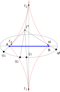
Figure 1: The set $\Pi(S)$ of an ellipse $S$ is the set of points within the interior of the area within the evolute, called, in this case an asteroid. It is indicated by the red line. It is the set of all points in $\Re^{2}$ for which the curvature of locally convex type takes a non zero value. The Divider of $S$ is the segment of the great axis within the closure of $\Pi(S)$. Its endpoints are the centers of osculating circles of maximum curvature.

If, on the other hand, $S$ is a curve in $\Re^{2}$ and is homeomorphic to $(0,\,1)$, $(0,\,1]$ or $[0,\,1]$, then $\Pi(S)$ is the area of $\Re^{2}$ toward which the evolute $E$ turns its convex side. A typical example is a parabola 2.

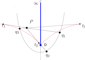
Figure 2: The evolute of a parabola is called a Neile’s parabola. The set $\Pi(S)$ lies within the area delimited by the red line, where the evolute turns its convex side. The Divider of a parabola is the part of its axis starting from the center of the osculating circle at the vertex of maximum curvature and going to infinity.

Proof.

By the theory developed in Bakopoulos1 (1), if $S$ is homeomorphic to a one - dimensional connected subset of a straight line, then a necessary and sufficient condition for the relation $p\in\Pi(S)$ to be valid, is that there is at least one line $p$ and $q$ normal to $S$, such that the distance $|p,q|$ of $p$ from $q$ is a local maximum of the distances of $p$ from points of $S$. If, on the other hand, $S$ is homeomorphic to $S^{(1)}$, then two line segments $|p,q_{1}|$, $|p,q_{2}|$, which must be local maxima of the distance of $p$ from points of $S$ Bakopoulos1 (1). For the above to hold, there must exist analogous tangent lines from $p$ to the evolute $E$ of $S$. For the distance of $p$ from a point $q$ of $S$ to be a local maximum, the point of contact $t$ of $pq$ with $E$ must lie between $p$ and $q$. The above statement can be true only if $p$ is at the convex side of $E$, so that the appropriate tangent or tangents may exist. ∎

Lemma III.5.

If $S$ is homeomorphic to $S^{(1)}$ and different from $S^{(1)}$, then from every point $p$ of $\Pi(S)$, there will be at least four tangents to $E$ from $p$. Correspondingly, they will be normal to $S$, by definition of involutes and evolutes. Two of them will define local minimum distances of $p$ from $S$ and two will define local maximum distances from $p$ to $S$ 1. Each one of then is tangent to $E$ at a point $t_{i}$, $i=1,2,3,4$, which is the center of an osculating circle of $S$ at a point $q\in S$. The lines defining local maxima and minima of distance will alternate in succession as they meet $S$. If, on the other hand, $S$ is a curve in $\Re^{2}$ and is homeomorphic to $(0,1)$, $(0,1]$ or $[0,1]$ but is not a straight line subset, then there will be at least three tangents from $p$ to $E$. Two of them will define local minimum distances of $p$ from $S$ and one of them will define a local maximum distance. The line defining a local maximum will lie between the other two lines.

Theorem III.6.

If a tangent is defined from $p\in\Pi(S)$ to the evolute $E$ of $S$, being normal to $S$ at $q$, then the points $p^{\prime}$ on the straight line $(p,q)$ have the following properties: If a point $p^{\prime}$ lies on the far side of $q$ relative to the center $t$ of the osculating circle, the distance $|p,q|$ is a local minimum, in the sense that if a small enough open neighborhood of $q,N(q)$, is considered on $S$, then $\forall q^{\prime}\in\Pi(S)$ the relation: $|p,q|<|p,q^{\prime}|$ holds.

The same is true if $p$ lies between $q$ and $t$. If $p$ is at the far side of $t$ relative to $q$, in other words if $t$ is between $p$ and $q$ then the distance $|p,q|$ is a local maximum, meaning that, if a small enough open neighborhood of $q,N(q)$, is considered on $S$, then $\forall q^{\prime}\in\Pi(S)$ the relation: $|p,q|>|p,q^{\prime}|$ holds. Furthermore, if $p=t$, then if $t$ is the center of an osculating circle with maximum curvature, as described above, the relation $|t,q|<|t,q^{\prime}|$ holds. If $t$ is the center of an osculating circle of minimum curvature, the relation $|t,q|>|t,q^{\prime}|$ holds. Finally, if $t$ is the center of an osculating circle with neither maximum nor minimum curvature, the distance $|t,q|$ is neither maximum nor minimum. If any neighborhood $N(q)$ is considered on $S$, however small, the points $q^{\prime}$ in $N(q)$ for which the osculating curvature is larger than that in $q$ will lie outside the osculating circle at $q$, while the points $q^{\prime}$ where the osculating curvature is larger than that of $q$ will lie within the osculating circle ay $q$. The above results are well known facts from differential geometry. An osculating circle of a curve at a point $p$ is in contact of at least the second degree with the curve at $p$. If the curvature is locally maximum or minimum, then the contact is at least of the third degree. If the curvature is locally a maximum, then the curve lies outside the osculating circle at a neighbourhood of $p$. If the curvature is a local minimum, then the curve lies inside the osculating circle at a neighbourhood of $p$. In ordinary cases, i.e., when the contact at the point in question does not happen to be of an order higher than the second, the circle of curvature will not merely touch the curve, but will also cross it Taylor (17). These results can be naturally extended to curves and surfaces in three dimensions Sherbrooke1 (6, 8, 17).

Now an important Theorem will be presented:

Theorem III.7.

Let $S$ be a curve in $\Re^{2}$, homeomorphic to $(0,1)$, twice continuously differentiable, unbounded, not containing arcs of constant curvature and with only one point $q_{0}$ of maximum curvature. The Divider of $S$ is contained in the closure of $\Pi(S)$, at the part of $\Re^{2}$ where its evolute $E$ turns its convex side. The end points of the Divider are cusps of the evolute $E$ of $S$, corresponding to maximum curvature of the relative osculating circles.

Proof.

If $S$ is as above, obviously the evolute $E$ will have two branches joining at a cusp $t$ and having a common tangent there. The cusp $t$ will be the center of an osculating circle of maximum osculating curvature. If a point $p\neq t$ belongs to the Divider, there will be exactly three straight line segments $|p,q_{1}|$, $|p,q_{2}|$, $|p,q_{3}|$, normal to $S$ and tangent to $E$. One of them, $|p,q_{2}|$, will define a local (and global) maximum distance of $p$ from $S$ and will lie among the other two. The other two distances, $|p,q_{1}|,|p,q_{3}|$, will be equal by definition of the Divider. Also, being equal to the radius of the supremum of disks having contact with $S$ at only one point, it will also be the infimum of the disks having more than one contact points with $S$. The set $B^{(2)}(p,|p,q_{2}|)\bigcap S$ will be disconnected, containing only two distinct points $q_{1}$ and $q_{3}$. Therefore, $p\in\Pi(S)$ On the other hand, let the cusp t of $E$ be considered. It will be the center of the circle of maximum osculating curvature of $S$ at $q$. As such, by Lemma III.4 and III.6, it will also be the center of the maximum disk contacting $S$ at its single point $q$. Therefore, the disk having $t$ as a center and $|t,q|$ as a radius, will define the contact curvature of $S$ at $q$. The cusp t will belong to the Divider and since it will not belong to $\Pi(S)$, it will be an end point of the Divider. The osculating disk will not intersect $S$ at any other point, since $S$ has only one point of maximum curvature. Similar results can be easily proved for more general curves, homeomorphic to $(0,1]$, $[0,1]$, $S^{(1)}$, lines which are receptive of a normal at each point but their osculating curvature function is piece by piece continuous, or even disconnected sets of curves. The above results do not hold only in cases where S has points of self intersection 3. ∎

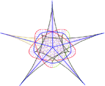
Figure 3: A hypotrochoid $S$ and its evolute are the best example of an exception to the rules for curves without double points. Note that vertices of a curve correspond to its evolute cusps. The lines are radii of tangent circles. The area inside the evolute defines the set $\Pi(S)$ of the hypotrochoid $S$. The points at the interior have a positive curvature of locally convex type. The Divider interior points are contained in the set $\Pi(S)$. The cusps of the evolute corresponding to the maximum curvature points of the hypotrochoid, are not end points of the Divider. This is because the osculating disks at the maximum curvature points are larger than the corresponding maximal disks in the same points. The cross points of the hypotrochoid are points of the Divider with zero radius maximal disks, having infinite curvature of locally convex type. The interior of the smaller curved asteroid decagon inside the hypotrochoid is the area where the disks defining the curvature of locally convex type may have an intersection with the hypotrochoid with five distinct connected components. As a special case, the central junction point of the Divider, situated at the center of the Figure, is the starting point of five branches of the Divider, these being straight lines radiating from the junction to each cross point of the hypotrochoid. There are five more branches of the Divider, uniting the hypotrochoid cross points within each outer lobe of the hypotrochoid. The last five branches of the Divider are straight lines starting from each cross point of the hypotrochoid, passing through the corresponding cusp of the evolute which is a center of a minimum curvature osculating disk and going on to infinity. In this case the Divider is a multiply connected graph containing singular points of zero contact curvature due to the existence of analogous singularities (cross points) in the hypotrochoid.

All the above statements can be verified by the Divider defining equations presented below: Let a curve $S$ in be defined by the parametric functions:

$$x_{1} = x_{1}(t)$$ (5)

$$x_{2} = x_{2}(t)$$ (6)

Given any value $t_{1}$ of the defining parameter of $S$, the following quantities will be calculated, by the equations and inequalities presented below: $x_{1}(t_{1}),\,x_{2}(t_{1}),\,t_{2},$ $x_{1}(t_{2}),\,x_{2}(t_{2}),\,x_{10},\,x_{20}$.

$$x_{1} = x_{1}(t_{1})$$ (7)

$$x_{2} = x_{2}(t_{1})$$ (8)

$$x_{1} = x_{1}(t_{2})$$ (9)

$$x_{2} = x_{2}(t_{2})$$ (10)

$$(x_{1}(t_{1})-x_{10})\frac{dx_{1}(t_{1})}{dt_{1}}+(x_{2}(t_{1})-x_{20})\frac{dx_{2}(t_{1})}{dt_{1}} = 0$$ (11)

$$(x_{1}(t_{2})-x_{10})\frac{dx_{1}(t_{2})}{dt_{2}}+(x_{2}(t_{2})-x_{20})\frac{dx_{2}(t_{2})}{dt_{2}} = 0$$ (12)

$$(x_{1}(t_{1})-x_{10})^{2}+\left(x_{2}(t_{1})-x_{20}\right)^{2} = (x_{1}(t_{2})-x_{10})^{2}+\left(x_{2}(t_{2})-x_{20}\right)^{2}$$ (13)

$$0<(x_{1}(t_{1})-x_{10})\frac{d^{2}x_{1}(t_{1})}{dt_{1}^{2}}+\left(\frac{dx_{1}(t_{1})}{dt_{1}}\right)^{2}+(x_{2}(t_{1})-x_{20})\frac{d^{2}x_{2}(t_{1})}{dt_{1}^{2}}+\left(\frac{dx_{2}(t_{1})}{dt_{1}}\right)^{2}$$ (14)

$$0<(x_{1}(t_{2})-x_{10})\frac{d^{2}x_{1}(t_{2})}{dt_{2}^{2}}+\left(\frac{dx_{1}(t_{2})}{dt_{1}}\right)^{2}+(x_{2}(t_{2})-x_{20})\frac{d^{2}x_{2}(t_{2})}{dt_{2}^{2}}+\left(\frac{dx_{2}(t_{2})}{dt_{2}}\right)^{2}$$ (15)

There are important cases where the equations:

$$(x_{1}(t_{1})-x_{10})\frac{d^{2}x_{1}(t_{1})}{dt_{1}^{2}}+\left(\frac{dx_{1}(t_{1})}{dt_{1}}\right)^{2}+(x_{2}(t_{1})-x_{20})\frac{d^{2}x_{2}(t_{1})}{dt_{1}^{2}}+\left(\frac{dx_{2}(t_{1})}{dt_{1}}\right)^{2}=0$$ (16)

$$(x_{1}(t_{2})-x_{10})\frac{d^{2}x_{1}(t_{2})}{dt_{2}^{2}}+\left(\frac{dx_{1}(t_{2})}{dt_{1}}\right)^{2}+(x_{2}(t_{2})-x_{20})\frac{d^{2}x_{2}(t_{2})}{dt_{2}^{2}}+\left(\frac{dx_{2}(t_{2})}{dt_{2}}\right)^{2}=0$$ (17)

are true and yet the distances $|p,q_{1}|$, $|p,q_{2}|$ are local minima. In that case, the sign and order of the lowest, in order succession, nonzero derivative decides if $|p,q_{1}|$ and $|p,q_{2}|$ are local maxima or local minima of the distances of p from the points $q$ of $S$. This simplified version of minimum distance conditions is given here for reasons of space. In cases of curves or surfaces with boundaries, the existence of local maxima or minima of the distance of $p$ from $S$ is not necessarily connected with the existence of normals from $p$ to $S$. In such cases, minimum or maximum distances may lie on the boundary of $S$, in which case a set of relations analogous to 1, 2–3, 7 may not exist, or may yield only partial results, in the creation of the Divider. In such cases, the algorithms for the creation of the Divider should use procedures not entirely based on such well defined and solvable equations.

As $t_{1}$ spans $S$, the coordinates $x_{10}$, $x_{20}$, of the Divider are calculated, as functions of the variable $t_{1}$.

Let a curve $S$ in $\Re^{2}$, homeomorphic but not similar to $S(1)$, be considered. The above equations are consistent with the definition of maximal disks Sherbrooke1 (6, 7, 8, 9, 10, 13). The maximal disks definition and the Divider definition are equivalent as long as the Euclidean metric 1 is used. The definition of contact disks and maximal disks as stated in this work and in Aggarwal (5) are not equivalent to the traditional definition of maximal disks, if one of the other metrics, 2 and 3, is used.

The above equations 7 to 13 are designed to find the coordinates $x_{10}$, of all points $x_{1}(t_{1})$ and $x_{2}(t_{1})$ which belong to the Divider of $S$. The procedure is as follows. If a value $t_{1}$ of the parameter $t$ in the relations 7 and 8 defining $S$ is given, then, by 7 and 8, a point $q_{1}$ with coordinates $x_{1}(t_{1})$ and $x_{2}(t_{1})$ will be defined. Equations 9 and 10 define a new value $t_{2}$ of $t$ and the coordinates $x_{1}(t_{2})$ and $x_{2}(t_{2})$ of a corresponding point $q_{2}$, with appropriate properties designated by the following equations. The rest of the equations, 12 to 13, define the coordinates $x_{01}$ and $x_{02}$ of a point $p\in\Re^{2}$ which, as stated above, will belong to the Divider of S. Equation 11 signifies that $|p,q_{1}|$ is normal to $S$. Equation 12 signifies that $|p,q_{2}|$ is normal to $S$. Equation 13 signifies that $|p,q_{1}|=|p,q_{2}|$. Finally, inequalities 14, 15 certify that $|p,q_{1}|$ and $|p,q_{2}|$ are local minima of the distances of $p$ from the points of $S$.

The above equations can be easily extended to curves and surfaces in $\Re^{3}$. Other, more general geometric objects in abstract metric spaces may be defined by similar equations. By the theory of curves and surfaces, if $S$, be it a curve or a surface in $\Re^{2}$ or $\Re^{3}$, is unbounded in the topological sense and, furthermore, has no boundary points by its intrinsic topology Spivak (18), the set of equations 7 to 13 has at least one solution. In $\Re^{2}$, this would mean a minimum of distances $|p,q|$, $q\in S$, if one of the inequalities 14 or 15 would hold. Conversely, if none of the above inequalities holds and the solution yields a local maximum, there will be at least two more solutions, both defining local minima of distances $|p,q|$, $q\in S$, at points $q_{1}$, $q_{2}$. By 13, $|p,q_{1}|=|p,q_{2}|$. Then the point $p$ would belong to the Divider of $S$. Analogous results hold for bounded curves or surfaces, homeomorphic to $S(1)$ or $S(2)$ but not having everywhere constant curvature. A special case is that of a center $c$ of an osculating circle of constant curvature at every point $q^{\prime}$ on $N(q)$. In that case the following are true:

1. S contains a compact, connected circular arc $Q$ with $c$ as its center.

2. Every contact direction for every $q\in Q$ passes through c.

3. The disk of the osculating circle is the supremum of the disks which have with $S$ only one common point $q$, belonging to $Q$. The center $c$ of the osculating circle for the points $q$ of $Q$ is the corresponding point for the Divider for $Q$.

All the above results are presented here without proof, since they are well known from classical differential geometry.

IV Discussion and conclusions

In the above, the main contribution is the definition of a new skeleton concept, the Divider set. Being in some sense the reverse of the maximal disk definition, the definition of the Divider is given in reference to the points of a curve or surface. This may or may not be the boundary of an area, finite or infinite. The definition and the construction of a maximal contact disk will start from a point on the curve or surface. On the other hand, the classical definition of Blum, has to do with maximal inscribed disks. Therefore, Therefore the algorithms creating it will be in principle more efficient from algorithms referring to all points inside a given enclosed area, as are the grassfire or wave front algorithms and most maximal disks algorithms these authors are aware of Sherbrooke1 (6, 7, 8, 9, 10, 11, 12, 13, 14). This seems to be the case in the first attempts for a Divider creating algorithm by the use of the defining equations using the Euclidean metric 1, 2, 3, and also in the case of the discrete lattice Aggarwal (5). In that last case, the maximum coordinate metric is used. In most cases in the literature, for a small sample see Tsang1 (11, 12, 14), the Euclidean metric is used for the creation of skeletons, even in a discrete lattice environment.

The maximal disk definition, as mentioned above, is not well suited for the maximum coordinate metric. On the other hand the Divider definition can be naturally modified Aggarwal (5) for a discrete lattice environment. The result is a connected set of cells, having at most a two cells width wherever the distance of the lines is an even number of cells. This is a well known problem with discrete lattices Tsang1 (11, 12, 14) and there are many issues to be discussed. One of them, arguably the most important, is the creation of a skeleton suitable for image compression and more or less faithful restoration Sherbrooke1 (6, 8, 9, 10). The authors of this work are of the opinion that in some cases reproduction of a faithful image requires that all skeleton pixels should be kept and no further thinning algorithm should be applied. In other cases, like OCR, where no faithful reconstruction of the image is required but the objective is the extraction and preservation of some important features of the initial image, there are some simple thinning algorithms that can be applied with good results Aggarwal (5).

In general, the Divider seems to work in a satisfactory manner for the applications of interest to the authors, for example OCR and robotic navigation in enclosed environments, among others. To conclude, by the work so far, the Divider concept seems to have some distinct advantages compared with many other state of the art skeletonization methods. It has a precise mathematical definition, easily implemented algorithms for two and three dimensional Euclidean spaces utilizing the Euclidean metric, as well as discrete lattice spaces, utilizing the maximum coordinate metric. It seems to be promising for many applications, although further testing and comparison with alternate methods is still to be done in future work. It has especially promising attributes in specific interesting applications, such as handwritten text recognition and robotic navigation, among others.