Boundary cliques, clique trees and perfect sequences of maximal cliques of a chordal graph

Abstract

We characterize clique trees of a chordal graph in their relation to simplicial vertices and perfect sequences of maximal cliques. We investigate boundary cliques defined by Shibata[23] and clarify their relation to endpoints of clique trees. Next we define a symmetric binary relation between the set of clique trees and the set of perfect sequences of maximal cliques. We describe the relation as a bipartite graph and prove that the bipartite graph is always connected. Lastly we consider to characterize chordal graphs from the aspect of non-uniqueness of clique trees.

Keywords and phrases : boundary clique, chordal graph, clique tree, maximal clique, minimal vertex separator, perfect sequence, simplicial vertex.

1 Introduction

Chordal graphs are useful for many practical problems. For example they arise in the context of sparse linear systems (Rose[22]), relational data bases (Bernstein and Goodman[2]), positive definite completions (e.g. Grone et al.[13], Fukuda et al.[8], Waki et al.[25]). In statistics, graphical models have received increasing attention (e.g. Whittaker[26], Lauritzen[20]). The decomposable graphical models determined by chordal graphs are particularly convenient and have been extensively studied by many authors (e.g. Dobra[7], Geiger, Meek and Sturmfels[11], Hara and Takemura[14], [15]). In view of these applications it is important to study properties of chordal graphs.

In this article we focus on characterizations of clique trees for a chordal graph. A clique tree is an intersection graph representation of a chordal graph and in general there are many clique trees for a chordal graph. Clique trees are very important from the algorithmic point of view for many techniques based on chordal graphs. They have been used to solve domination problems on directed path graphs (Booth and Johnson[3]). They also provide efficient algorithms for probability propagation in graphical models (e.g. Jensen[17]).

The purpose of this article is to characterize the set of clique trees in three ways. We first address properties of boundary cliques defined by Shibata[23] which form an important subclass of simplicial cliques. Shibata[23] showed that if a maximal clique $C$ is an endpoint of some clique tree, then $C$ is a boundary clique. We show that the converse of this fact holds and give some characterizations of endpoints of clique trees by using the notion of boundary cliques. In this paper we also use an alternative terminology and call a boundary clique simply separated, because a boundary clique meets a single minimal vertex separator. The characterization of endpoints of clique trees is essential for proving theoretical facts on chordal graphs by induction on the number of maximal cliques.

Secondly we consider the relation between the set of clique trees and the set of perfect sequences of maximal cliques. Lauritzen[20] presents two (randomized) algorithms, one of which generates a clique tree from a perfect sequence given as an input and the other generates a perfect sequence of maximal cliques from a clique tree given as an input. Based on these algorithms, we can define a symmetric binary relation between the set of clique trees and the set of perfect sequences of maximal cliques. In this article we consider to describe this relation using a bipartite graph. We prove that the bipartite graph is connected for every chordal graph. This result allows us to construct a connected Markov chain over the set of clique trees and the set of perfect sequences of maximal cliques of a given chordal graph. The Markov chain is potentially useful for optimizing over the set of clique trees or over the set of perfect sequences of maximal cliques. In the proof of the connectedness of the bipartite graph we use the induction on the number of maximal cliques and we can confirm the usefulness of our characterization of endpoints of clique tree by using the notion of boundary cliques.

Finally we consider the question of uniqueness of clique trees. As mentioned above a chordal graph may have many clique trees. As two extremes, there exists a chordal graph such that an arbitrary tree is a clique tree for it and there also exists a chordal graph such that the clique tree is unique. We derive a necessary and sufficient condition on chordal graphs for the arbitrariness and for the uniqueness of their clique trees.

The organization of this paper is as follows. In Section 2 we prepare notations and present some preliminary facts on the simplicial vertices, the clique trees and the perfect sequences of maximal cliques of a chordal graph. In Section 3 we consider boundary cliques and give some characterization of endpoints of clique trees in relation to boundary cliques. We also characterize a final maximal clique in a perfect sequence by using the notion of boundary cliques. In Section 4 we define a symmetric binary relation between the set of clique trees and the set of perfect sequences of maximal cliques and consider to describe the relation by a bipartite graph. In particular we prove that the bipartite graph is connected. In Section 5 we derive the necessary and sufficient condition for the arbitrariness and the uniqueness of clique trees. We end the paper with some concluding remarks in Section 6.

2 Preliminaries

In this section we prepare notations, definitions and some basic results on chordal graphs required in the subsequent sections. Throughout this paper we assume that the undirected graph $G$ is a connected chordal graph, because for a general chordal $G$ it suffices to consider clique trees separately for each connected component.

2.1 Notations and definitions

Let ${V}$ be the set of vertices in $G$. Denote by ${\cal C}$ and ${\cal S}$ the set of maximal cliques and the set of minimal vertex separators in $G$, respectively. It is well known that $G$ is chordal if and only if every minimal vertex separator is a clique (Dirac[6]). Define $n=|{V}|$ and $K=|{\cal C}|$. For a subset of vertices ${V}^{\prime}\subset{V}$, the subgraph induced by ${V}^{\prime}$ is denoted by $G({V}^{\prime})$. Let ${\cal C}({V}^{\prime})={\cal C}(G({V}^{\prime}))$ and ${\cal S}({V}^{\prime})={\cal S}(G({V}^{\prime}))$ denote the set of the maximal cliques and the set of minimal vertex separators of $G({V}^{\prime})$. For a subset of maximal cliques ${\cal C}^{\prime}\subset{\cal C}$, denote ${V}({\cal C}^{\prime})=\bigcup_{C\in{\cal C}^{\prime}}C\subseteq V$. Here a maximal clique $C$ is considered to be a subset of ${V}$. In this article we use $\subset$ for a proper containment and $\subseteq$ for a containment with equality allowed.

For a vertex ${v}\in{V}$, we denote by $N_{G}({v})$ the open adjacency set of ${v}$ in $G$, i.e. the set of all neighbors of ${v}$ in $G$, and by $N_{G}[{v}]$ the closed adjacency set of ${v}$ in $G$, i.e. $N_{G}[{v}]=N_{G}({v})\cup\{{v}\}$. For a subset of vertices ${V}^{\prime}\subset{V}$, define $N_{G}({V}^{\prime})$ and $N_{G}[{V}^{\prime}]$ as follows,

$$N_{G}({V}^{\prime})=\bigcup_{{v}\in{V}^{\prime}}N_{G}({v})\setminus{V}^{\prime},\quad N_{G}[{V}^{\prime}]=\bigcup_{{v}\in{V}^{\prime}}N_{G}[{v}].$$

A tree $T=({\cal C},{\cal E})$ is called a clique tree for $G$ if for any two maximal cliques $C_{1}\in{\cal C}$ and $C_{2}\in{\cal C}$ and any $C_{3}\in{\cal C}$ on the unique path in $T$ between $C_{1}$ and $C_{2}$ it holds that

$$C_{1}\cap C_{2}\subseteq C_{3}.$$

This is known as the junction property of $T$. It is well known that a clique tree exists if and only if $G$ is chordal (e.g. Buneman[4] and Gavril[10]). For two maximal cliques $C_{1}$ and $C_{2}$ such that $(C_{1},C_{2})\in{\cal E}$, there exists a minimal vertex separator $S\in{\cal S}$ such that $C_{1}\cap C_{2}=S$. Hence each edge of $T$ corresponds to a minimal vertex separator(e.g. Ho and Lee[16]). For a subset ${\cal C}^{\prime}\subset{\cal C}$, denote the subtree of $T$ induced by ${\cal C}^{\prime}$ by $T({\cal C}^{\prime})$. If $T({\cal C}^{\prime})$ is connected, then $T({\cal C}^{\prime})$ also satisfies the junction property. In this case the induced subgraph $G({V}({\cal C}^{\prime}))$ is also chordal with ${\cal C}({V}({\cal C}^{\prime}))={\cal C}^{\prime}$.

For a (not necessarily maximal) clique $D$ let

$${\cal C}_{\uparrow D}=\{C\in{\cal C}\mid D\subseteq C\}$$

denote the set of maximal cliques containing $D$. Then the junction property can be alternatively expressed that ${\cal C}_{\uparrow D}$ induces a connected subtree of $T$ for every clique $D$. Let $\tilde{\cal C}$ denote the set of all cliques of $G$. Kumar and Madhavan[18] showed that it is sufficient to consider ${\cal C}_{\uparrow S}$ for each minimal vertex separator $S\in{\cal S}$, i.e.,

$$\{{\cal C}_{\uparrow S}\mid S\in{\cal S}\}\qquad\text{and}\qquad\{{\cal C}_{\uparrow D}\mid D\in\tilde{\cal C}\}$$

induce the same set of connected subtrees of a clique tree.

As already mentioned, there may be many clique trees for $G$. Ho and Lee[16] and Kumar and Madhavan[18] provided efficient algorithms to enumerate all clique trees. Ho and Lee[16] gave the number of the clique trees of chordal graphs explicitly. For $S\in{\cal S}$, let $\Gamma_{1},\dots,\Gamma_{M}$ be the connected components of $G({V}\setminus S)$. Define ${\cal M}_{S}$ and ${\cal C}_{\uparrow S}(\Gamma_{m}\cup S)$, $m=1,\dots,M$, by

$${\cal M}_{S}=\{m\mid N_{G}(\Gamma_{m})=S\},\quad{\cal C}_{\uparrow S}(\Gamma_{m}\cup S)=\{C\in{\cal C}\mid C\subseteq\Gamma_{m}\cup S,C\supset S\}.$$ (1)

Let ${\cal T}$ be the set of all clique trees for $G$. Ho and Lee[16] showed that the number of the clique trees for $G$ is expressed by

$$|{\cal T}|=\prod_{S\in{\cal S}}\left[\left(\sum_{m\in{\cal M}_{S}}|{\cal C}_{\uparrow S}(\Gamma_{m}\cup S)|\right)^{|{\cal M}_{S}|-2}\cdot\prod_{m\in{\cal M}_{S}}|{\cal C}_{\uparrow S}(\Gamma_{m}\cup S)|\right].$$ (2)

We consider to characterize the chordal graphs from the aspect of the arbitrariness and the uniqueness of clique trees in Section 5.

Other important characterizations of the clique trees are addressed in Bernstein and Goodman[2] and Shibata[23] etc.

A vertex ${v}\in{V}$ is called simplicial if $N_{G}({v})$ is a clique. Dirac[6] showed that any chordal graph with at least two vertices has at least two simplicial vertices and that if the graph is not complete, these can be chosen to be non-adjacent. A bijection $\sigma:\{1,\dots,n\}\rightarrow{V}$ is called a perfect elimination scheme of vertices of $G$ if $\sigma(i)$ is a simplicial vertex in $G(\bigcup_{j=i}^{n}\{\sigma(j)\})$. It is well known that $G$ is chordal if and only if $G$ contains a perfect elimination scheme. The perfect elimination scheme is used to determine whether a given graph is chordal. Linear time algorithms to generate a perfect elimination scheme are proposed in Tarjan and Yannakakis[24] and Golumbic[12] etc.

For a maximal clique $C$, let ${\rm Simp}(C)$ denote the set of simplicial vertices in $C$ and let ${\rm Sep}(C)$ denote the set of non-simplicial vertices in $C$. Then $C={\rm Simp}(C)\cup{\rm Sep}(C)$ is a partition (disjoint union) of $C$. As shown below in Lemma 2.1,

$${\rm Sep}(C)=C\cap{V}({\cal C}\setminus\{C\})=C\cap\bigcup_{S\in{\cal S}}S.$$

We call ${\rm Simp}(C)$ the simplicial component of $C$ and ${\rm Sep}(C)$ the non-simplicial component of $C$, respectively. We call a maximal clique $C$ simplicial if ${\rm Simp}(C)\neq\emptyset$. Note that for brevity of terminology in this paper we simply say “simplicial clique” instead of “simplicial maximal clique”.

Denote the maximal cliques in $G$ by $C_{k}$, $k=1,\dots,K$. Define ${\cal I}=\{1,\dots,K\}$. For the permutation $\pi:{\cal I}\rightarrow{\cal I}$, define $H_{\pi(k)}$, $k=1,\dots,K$, and $S_{\pi(k)}$, $k=2,\dots,K$, by

$$H_{\pi(k)}=C_{\pi(1)}\cup\cdots\cup C_{\pi(k)},\quad S_{\pi(k)}=H_{\pi(k-1)}\cap C_{\pi(k)},$$ (3)

respectively. The sequence of the maximal cliques $C_{\pi(1)},C_{\pi(2)},\dots,C_{\pi(K)}$ is a perfect sequence of the maximal cliques if every $S_{\pi(k)}$ is a clique and there exists $k^{\prime}<k$ such that $S_{\pi(k)}\subset C_{\pi(k^{\prime})}$ for all $k\geq 2$. This is known as the running intersection property of the sequence. There exists a perfect sequence of maximal cliques if and only if $G$ is chordal and then $S_{\pi(k)}\in{\cal S}$ for all $k$ and

$$\{S_{\pi(2)},\dots,S_{\pi(K)}\}={\cal S},$$ (4)

where the same minimal vertex separator $S$ may be repeated several times on the left-hand side (e.g. Lauritzen[20]). Define the multiplicity $\nu(S)$ of $S\in{\cal S}$ by

$$\nu(S)=\#\{k\mid S_{\pi(k)}=S,\;k=2,\dots,K\}.$$

It is known that $\nu(S)$ does not depend on $\pi$. It is also known that there exists a perfect sequence such that $C_{\pi(1)}=C_{k}$ for all $k=1,\dots,K$. We identify the sequence $C_{\pi(1)},C_{\pi(2)},\dots,C_{\pi(K)}$ with the permutation $\pi$ for simplicity for the rest of the paper. Denote the set of perfect sequences of $G$ by $\varPi$.

2.2 Some basic facts on chordal graphs

In this subsection we present some basic facts on chordal graphs required in the following sections in the form of series of lemmas. Many results of this section are not readily available in the existing literature. However they are of preliminary nature and we do not intend to claim originality of the results of this subsection. The readers may skip the proofs of the lemmas and refer to the lemmas when needed in checking proofs of our main results in the later sections.

We first state the following fundamental property of the simplicial vertices.

Lemma 2.1 (Hara and Takemura[14]).

The following three conditions are equivalent,

• ${v}\in{V}$ is simplicial ;

• there is only one maximal clique $C$ which includes ${v}$ ;

• ${v}\notin S$ for all $S\in{\cal S}$.

Note that from this lemma it follows that

$${V}({\cal C}\setminus\{C\})=V\setminus{\rm Simp}(C),\qquad\forall C\in{\cal C}.$$

Next we consider a relation between a beginning part of a perfect sequence of maximal cliques and a connected induced subtree of a clique tree. Let $C_{\pi(1)},\dots,C_{\pi(K)}$ be a perfect sequence of the maximal cliques. For $k<K$, the subsequence $C_{\pi(1)},\dots,C_{\pi(k)}$ also satisfies the running intersection property. Denote ${\cal C}_{\pi(k)}=\bigcup_{i=1}^{k}\{C_{\pi(i)}\}$. Then the induced subgraph $G({V}({\cal C}_{\pi(k)}))$ is a chordal graph with ${\cal C}({V}({\cal C}_{\pi(k)}))={\cal C}_{\pi(k)}$. Therefore we have the following lemma.

Lemma 2.2.

Suppose that ${\cal C}^{\prime}\subset{\cal C}$ and $|{\cal C}^{\prime}|=k$. There exists a clique tree such that the induced subtree $T({\cal C}^{\prime})$ is connected if and only if there exists a perfect sequence $\pi$ such that ${\cal C}^{\prime}={\cal C}_{\pi(k)}$.

We consider this relation once again in Section 4.

Lemma 2.3.

If $G$ is not complete, then $G({V}({\cal C}\setminus\{C\}))$ is connected.

Proof..

Since $G$ is connected ${\rm Sep}(C)\neq\emptyset$. Let ${v}\in{\rm Sep}(C)$. From (ii) in Lemma 2.1, ${v}$ is contained in at least two maximal cliques. Then ${v}\in{V}({\cal C}\setminus\{C\})$. Since the simplicial component is not a separator of $G$ from (iii) in Lemma 2.1, $G({V}({\cal C}\setminus\{C\}))$ is connected. ∎

For our proofs it is important to consider “small” minimal vertex separators. In particular we consider a minimal vertex separator $S\in{\cal S}$ which is minimal in ${\cal S}$ with respect to the inclusion relation. The following lemma concerns minimal vertex separators which are minimal in ${\cal S}$ with respect to the inclusion relation. Denote the connected components of $G({V}\setminus S)$ by $\Gamma_{1},\dots,\Gamma_{M}$.

Lemma 2.4.

Let $S\in{\cal S}$ be minimal in ${\cal S}$ with respect to the inclusion relation. Then

• ${\cal C}=\bigcup_{m=1}^{M}{\cal C}(\Gamma_{m}\cup S)$ is a disjoint union ;

• if $G(\Gamma_{m}\cup S)$ is not complete, then ${\cal S}(\Gamma_{m}\cup S)\subset{\cal S}$ ;

• there exists a perfect sequence $\pi$ such that the set of the first $|{\cal C}(\Gamma_{m}\cup S)|$ maximal cliques is ${\cal C}(\Gamma_{m}\cup S)$ for every $m=1,\dots,M$. Hence there exists a clique tree such that the subgraph of it induced by ${\cal C}(\Gamma_{m}\cup S)$ is connected.

The proof of this lemma is presented in the Appendix. With respect to (i) in this lemma, we note that if $S$ is not minimal in ${\cal S}$ with respect to the inclusion relation, then in general we only have ${\cal C}\subseteq\bigcup_{m=1}^{M}{\cal C}(\Gamma_{m}\cup S)$.

In the remaining two lemmas of this subsection we consider properties of the set of maximal cliques ${\cal C}_{\uparrow S}=\{C\in{\cal C}\mid C\supset S\}\subseteq{\cal C}$ containing a minimal vertex separator $S$.

Lemma 2.5.

Let $S_{1},S_{2}\in{\cal S}$ be minimal vertex separators. If $S_{1}\neq S_{2}$, then ${\cal C}_{\uparrow S_{1}}\neq{\cal C}_{\uparrow S_{2}}$.

Proof..

Suppose that ${\cal C}_{\uparrow S_{1}}={\cal C}_{\uparrow S_{2}}$. Then we have

$$\bigcap_{C\in{\cal C}_{\uparrow S_{1}}}C=\bigcap_{C\in{\cal C}_{\uparrow S_{2}}}C\supseteq S_{1}\cup S_{2}.$$

Since $S_{1}\neq S_{2}$, we can assume $S_{2}\setminus S_{1}\neq\emptyset$ without loss of generality. Then we have

$$\bigcap_{C\in{\cal C}_{\uparrow S_{1}}}C\setminus S_{1}=\bigcap_{C\in{\cal C}_{\uparrow S_{2}}}C\setminus S_{1}\supseteq S_{2}\setminus S_{1}\neq\emptyset.$$

Hence there exists ${v}\in{V}({\cal C}_{\uparrow S_{1}})$ such that ${v}\in C\setminus S_{1}$ for all $C\in{\cal C}_{\uparrow S_{1}}$. This implies that $G({V}\setminus S_{1})$ is connected. This contradicts that $S_{1}$ is a minimal vertex separator of $G$. ∎

Define $K_{S}$ by $K_{S}=|{\cal C}_{\uparrow S}|$. Then we obtain the following lemma.

Lemma 2.6.

• ${\cal S}({V}({\cal C}_{\uparrow S}))\subseteq{\cal S}$ for every $S\in{\cal S}$.

• If $|{\cal S}({V}({\cal C}_{\uparrow S}))|=1$, then $\nu(S)=K_{S}-1$.

• If $|{\cal S}({V}({\cal C}_{\uparrow S}))|\geq 2$, then $S\subset S^{\prime}$ for all $S^{\prime}\neq S$, $S^{\prime}\in{\cal S}({V}({\cal C}_{\uparrow S}))$.

Proof..

(i) ${\cal C}_{\uparrow S}$ induces a connected subtree in any clique tree for $G$. Thus there exists a perfect sequence $\pi$ of ${\cal C}$ such that $\{C_{\pi(1)},\dots,C_{\pi(K_{S})}\}={\cal C}_{\uparrow S}$ from Lemma 2.2. Then

$${\cal S}({V}({\cal C}_{\uparrow S}))=\bigcup_{k=2}^{K_{S}}\{S_{\pi(k)}\}\subseteq{\cal S}.$$

(ii) Since $\{C_{\pi(K_{S}+1)},\dots,C_{\pi(K)}\}={\cal C}\setminus{\cal C}_{\uparrow S}$, $S_{\pi(k)}\neq S$ for $k>K_{S}$ from the running intersection property. Hence if $|{\cal S}({V}({\cal C}_{\uparrow S}))|=1$, then $\nu(S)=K_{S}-1$.

(iii) Let ${\cal C}_{\uparrow(S\cup S^{\prime})}$ be the set of maximal cliques in ${\cal C}_{\uparrow S}$ which include $S^{\prime}$. Then

$$\bigcap_{C\in{\cal C}_{\uparrow(S\cup S^{\prime})}}C\supseteq S\cup S^{\prime}.$$

Hence if $S\setminus S^{\prime}\neq\emptyset$, $G({V}({\cal C}_{\uparrow(S\cup S^{\prime})})\setminus S^{\prime})$ is connected, which implies that $G({V}({\cal C}_{\uparrow S})\setminus S^{\prime})$ is also connected. This contradicts that $S^{\prime}\in{\cal S}({V}({\cal C}_{\uparrow S}))$. ∎

3 Boundary cliques and endpoints in clique trees

In this Section we first define boundary cliques according to Shibata[23]. We also introduce an alternative terminology of simply separated cliques and simply separated vertices, which seem to be more descriptive. Next we characterize endpoints of clique trees in their relation to boundary cliques.

3.1 Boundary cliques and their properties

Definition 3.1.

A simplicial clique $C$ is a boundary clique if there exists a maximal clique $C^{\prime}$ such that

$$\mathrm{Sep}(C)=C\cap C^{\prime}.$$ (5)

Then $C^{\prime}$ is called a dominant clique. We also call $C$ a simply separated clique, ${\rm Simp}(C)$ a simply separated component and the vertices in ${\rm Simp}(C)$ simply separated vertices.

Remark 3.1.

If $C$ is not simplicial, then $C={\rm Sep}(C)$ is a maximal clique and hence there does not exist a dominant clique for $C$. Therefore if (5) holds, $\mathrm{Simp}(C)$ has to be non-empty. It follows that the condition (5) alone guarantees that $C$ is simplicial and that $C$ is a boundary clique. Because of this fact we simply say “boundary clique”, “simply separated clique” or “simply separated vertex” instead of “simplicial boundary clique”, “simply separated simplicial clique” or “simply separated simplicial vertex”.

We now give two characterizations of boundary cliques.

Proposition 3.1.

If $G$ is not complete, the following three conditions are equivalent,

• $C$ is a boundary clique ;

• there exists $S\in{\cal S}$ satisfying

  $$\mathrm{Sep}(C)=S;$$ (6)

• $G({V}({\cal C}\setminus\{C\}))$ is a chordal graph with ${\cal C}({V}({\cal C}\setminus\{C\}))={\cal C}\setminus\{C\}$.

Proof..

(i) $\Rightarrow$ (ii)  Suppose that (5) holds. Since $C$ is the only maximal clique which includes $\mathrm{Simp}(C)$, $\mathrm{Sep}(C)$ separates $\mathrm{Simp}(C)$ and $C^{\prime}\setminus\mathrm{Sep}(C)$. On the other hand, for $D\subset\mathrm{Sep}(C)$, $G((C\cup C^{\prime})\setminus D)$ is connected. This implies that $\mathrm{Simp}(C)$ and $C^{\prime}\setminus\mathrm{Sep}(C)$ are connected in $G(V\setminus D)$. Hence $\mathrm{Sep}(C)\in{\cal S}$.

(i) $\Leftarrow$ (ii)  Suppose that (6) holds. Then there exist ${v}\in\mathrm{Simp}(C)$ and ${v}^{\prime}\in N_{G}(S)\setminus C$ such that $S$ is a minimal ${v}-{v}^{\prime}$ separator in $G$. Since $S\cup\{{v}^{\prime}\}$ is a clique, there exists a maximal clique $C^{\prime}\in{\cal C}$ satisfying $C^{\prime}\supseteq S\cup\{{v}^{\prime}\}$. Then $C\cap C^{\prime}=S$.

(i) $\Rightarrow$ (iii)  Assume that $C$ satisfies (5). Since $C^{\prime\prime}\subseteq{V}({\cal C}\setminus\{C\})$ for all $C^{\prime\prime}\in{\cal C}\setminus\{C\}$, we have ${\cal C}\setminus\{C\}\subseteq{\cal C}({V}({\cal C}\setminus\{C\}))$. Suppose that ${\cal C}\setminus\{C\}\subset{\cal C}({V}({\cal C}\setminus\{C\}))$. Then there exists $C^{\prime\prime}\in{\cal C}({V}({\cal C}\setminus\{C\}))$ such that $C^{\prime\prime}\notin{\cal C}\setminus\{C\}$. If $C^{\prime\prime}\nsubseteq C$, $C^{\prime\prime}\notin{\cal C}$ is also maximal in $G$. This contradicts that ${\cal C}$ is the set of all maximal cliques in $G$. Hence $C^{\prime\prime}\subset C$. Then $C^{\prime\prime}$ satisfies $C^{\prime\prime}=\mathrm{Sep}(C)$. Then from the maximality of $C^{\prime\prime}$ in ${\cal C}\setminus\{C\}$, there does not exist $C^{\prime}\in{\cal C}\setminus\{C\}$ such that $C^{\prime}\supseteq\mathrm{Sep}(C)$. This contradicts the assumption that $C$ satisfies (5). Therefore ${\cal C}({V}({\cal C}\setminus\{C\}))={\cal C}\setminus\{C\}$.

(i) $\Leftarrow$ (iii)  Suppose that $G({V}({\cal C}\setminus\{C\}))$ is a chordal graph with ${\cal C}({V}({\cal C}\setminus\{C\}))={\cal C}\setminus\{C\}$. $G({V}({\cal C}\setminus\{C\}))$ is connected from Lemma 2.3 and $C\cap{V}({\cal C}\setminus\{C\})$ is a clique. However for all $C^{\prime}\in{\cal C}\setminus\{C\}$, $C^{\prime}\nsubseteq C$ from the maximality of $C^{\prime}$. Thus $C\cap{V}({\cal C}\setminus\{C\})$ is not a maximal clique of $G({V}({\cal C}\setminus\{C\}))$. Hence there exists a maximal clique $C^{\prime}\in{\cal C}\setminus\{C\}$ such that $C^{\prime}\supset C\cap{V}({\cal C}\setminus\{C\})$ and then $C\cap{V}({\cal C}\setminus\{C\})=C\cap C^{\prime}$. ∎

As mentioned in the previous section, any chordal graph which is not complete has at least two non-adjacent simplicial components (Dirac[6]). Shibata[23] showed the stronger result that any chordal graph which is not complete has at least two non-adjacent boundary cliques. Strengthening this fact, we present the following proposition. Note that if $G$ is not complete, then $G$ contains at least one minimal vertex separator $S$ which is minimal in ${\cal S}$ with respect to the inclusion relation.

Proposition 3.2.

Suppose that $S$ is a minimal vertex separator which is minimal in ${\cal S}$ with respect to the inclusion relation. Let $\Gamma_{1},\dots,\Gamma_{M}$ be the connected components of $G({V}\setminus S)$. Then each $\Gamma_{m}$, $m=1,\dots,M$, contains at least one simply separated component in $G$.

Proof..

It suffices to show that $\Gamma_{1}$ contains a simply separated component. $G_{1}=G(\Gamma_{1}\cup S)$ is also chordal. If $G_{1}$ is complete, $N_{G}(\Gamma_{1})=S\in{\cal S}$. Hence $\Gamma_{1}={\rm Simp}(\Gamma_{1}\cup S)$ is simply separated also in $G$.

When $G_{1}$ is not complete, there exist two non-adjacent simply separated cliques in $G_{1}$. Since $S$ is a clique, at least one of them does not include $S$. Suppose that $C\in{\cal C}_{1}={\cal C}(\Gamma_{1}\cup S)$ is simply separated in $G_{1}$ satisfying that the simplicial component of $C$ in $G_{1}$ does not include $S$. Then there exists $C^{\prime}\in{\cal C}_{1}$ such that

$$C\cap{V}({\cal C}_{1}\setminus\{C\})=C\cap C^{\prime}.$$

From (i) in Lemma 2.4, ${\cal C}_{1}\subset{\cal C}$. For all $C_{m}\in{\cal C}\setminus{\cal C}_{1}$, $C$ and $C^{\prime}$ satisfies

$$C\cap C_{m}\subset C\cap C^{\prime}.$$

Hence we have

$$C\cap C^{\prime}=C\cap{V}({\cal C}\setminus\{C\}).$$

Thus $C$ is simply separated also in $G$. ∎

Figure 1 presents two graphs with four and three maximal cliques. The set of the simplicial vertices in the graph in Figure 1-(i) and (ii) are $\{1,4,5,7\}$ and $\{1,4,5\}$, respectively. Among the simplicial vertices, the vertex 4 is not simply separated in both 1-(i) and 1-(ii). All other vertices are simply separated. As we will mention in Section 5, the clique trees for both of the graphs are uniquely defined as in Figure 2. Let $C_{v}$ denote the unique maximal clique containing ${v}$. In the graphs every clique contains a simplicial vertex. However $C_{4}$ is not an endpoint in both graphs.

In the literature other classifications of simplicial vertices have been discussed. The class of strongly simplicial vertices are an important subclass of the simplicial vertices. Following the definition of Agnarsson and Halldórsson[1], we define a strongly simplicial component as follows.

(i)                                                 (ii)

Figure 1: Chordal graphs with four and three maximal cliques

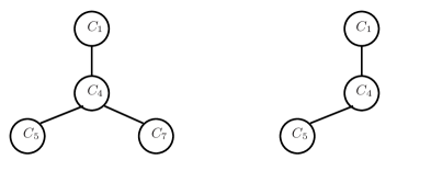
(i)                                                 (ii)

Figure 2: The clique trees of the graphs in Figure 1

Definition 3.2 (Strongly simplicial cliques (Agnarsson and Halldórsson[1])).

A simplicial clique $C$ is strongly simplicial if

$$\{N_{G}[{v}]\mid{v}\in N_{G}[{\rm Simp}(C)]\}$$

is a linearly ordered set with respect to the inclusion relation. In this case ${\rm Simp}(C)$ is called a strongly simplicial component and the vertices ${v}\in{\rm Simp}(C)$ are said to be strongly simplicial.

If $G$ contains a perfect elimination scheme $\sigma$ such that $\sigma(i)$ is a strongly simplicial vertex in $G(\bigcup_{j=i}^{n}\{\sigma(i)\})$, $G$ is called strongly chordal. The strongly chordal graphs are an important subclass of the chordal graphs because they yield polynomial time solvability of the domatic set and the domatic partition problems. Since Farber[9] first defined strongly chordal graphs, they have been studied by many authors (e.g. Chang and Peng[5], Kumar and Prasad[19]).

We now show that a strongly simplicial clique is simply separated.

Proposition 3.3.

If $C$ is a strongly simplicial clique, then it is simply separated.

Proof..

Suppose that

$$N_{G}({\rm Simp}(C))=\{{v}_{1},{v}_{2},\dots,{v}_{m}\},\quad N_{G}[{v}_{1}]\subseteq N_{G}[{v}_{2}]\subseteq\cdots\subseteq N_{G}[{v}_{m}].$$

Then

$$N_{G}[{v}_{1}]\cap N_{G}[{v}_{2}]\cap\cdots\cap N_{G}[{v}_{m}]=N_{G}[{v}_{1}].$$ (7)

Since ${v}_{1}$ belongs to at least two maximal cliques from (ii) in Lemma 2.1, we have $N_{G}[{v}_{1}]\setminus C\neq\emptyset$. Suppose that ${v}^{\prime}\in N_{G}[{v}_{1}]\setminus C$. From (7) and the fact that ${\rm Simp}(C)$ is simplicial, we have $N_{G}({\rm Simp}(C))\cap N_{G}({v}^{\prime})=\{{v}_{1},\dots,{v}_{m}\}=N_{G}({\rm Simp}(C))$. Since any vertices in ${\rm Simp}(C)$ and ${v}^{\prime}$ are not adjacent to each other, $\{{v}_{1},\dots,{v}_{m}\}$ is a minimal ${v}-{v}^{\prime}$ separator for ${v}\in{\rm Simp}(C)$. ∎

The converse of this proposition does not hold from Figure 1. Table 1 presents strongly, simply separated and not simply separated simplicial vertices for the graphs in Figure 1. We see the difference between each class.

Table 1: Simplicial vertices for the graph in Figure 1

	(i)	(ii)
Strongly simplicial	$\emptyset$	$1$, $5$
Simply separated but not strongly simplicial	$1$, $5$, $7$	$\emptyset$
Not simply separated	$4$	$4$

3.2 Relation between the simplicial components and the endpoints of clique trees

In this section we consider the characterization of endpoints of clique trees by using the notion of simply separated cliques. Shibata[23] showed that if a maximal clique $C$ is an endpoint of some clique tree, then it is simply separated. The following characterization of endpoints of cliques tree includes the converse of this fact.

Theorem 3.1.

If $C$ is simply separated, then there exists a clique tree $T$ such that $C$ is its endpoint. Furthermore if $C$ and $C^{\prime}$ are two simply separated cliques in two different connected components of $G({V}\setminus S)$, where $S$ is any minimal vertex separator which is minimal in ${\cal S}$ with respect to the inclusion relation, then there exists a clique tree $T$ such that $C$ and $C^{\prime}$ are its endpoints.

Proof..

When $K\leq 2$, there is nothing to prove. Then we assume that $K\geq 3$.

From Lemma 2.3 and (iii) in Proposition 3.1 $G({V}({\cal C}\setminus\{C\}))$ is a connected chordal graph with ${\cal C}({V}({\cal C}\setminus\{C\}))={\cal C}\setminus\{C\}$. Let $T^{\prime}=({\cal C}\setminus\{C\},{\cal E}^{\prime})$ be a clique tree of $G({V}({\cal C}\setminus\{C\}))$. Denote the dominant clique for $C$ by $C_{d}$. Consider the tree $T=({\cal C},{\cal E})$, where ${\cal E}={\cal E}^{\prime}\cup(C,C_{d})$. Then $C$ is an endpoint of $T$. For $C_{1}\in{\cal C}\setminus\{C\}$, let $C_{2}$ be any maximal clique on the unique path between $C$ and $C_{1}$. From the junction property of $T^{\prime}$, we have

$$C_{2}\supset(C_{1}\cap C_{d})\supset C\cap(C_{1}\cap C_{d})=(C\cap C_{1})\cap(C\cap C_{d})=C\cap C_{d}.$$

Hence $T$ also satisfies the junction property.

We move on to prove the second statement. Let $S$ a minimal vertex separator which is minimal in ${\cal S}$ with respect to the inclusion relation and let $\Gamma_{1},\dots,\Gamma_{M}$ be the connected components of $G({V}\setminus S)$. Let $\Gamma_{m}\supseteq C$ and $\Gamma_{m^{\prime}}\supseteq C^{\prime}$. Denote $S_{m}=\mathrm{Simp}(C)$ and $S_{m^{\prime}}=\mathrm{Simp}(C^{\prime})$, respectively. Denote the dominant cliques for $C$ and $C^{\prime}$ by $C_{m}$ and $C_{m^{\prime}}$, respectively. From (ii) in Proposition 3.1, we have

$$C\cap C_{m}=S_{m},\quad C^{\prime}\cap C_{m^{\prime}}=S_{m^{\prime}}$$ (8)

Since $C$ and $C^{\prime}$ belong to different connected components, $C\cap C^{\prime}\subseteq S$.

We first consider the case where $C\cap C^{\prime}\subset S$. Then $C\cap C^{\prime}$ is not a minimal vertex separator of $G$ from the minimality of $S$ in ${\cal S}$ with respect to the inclusion relation. If $C_{m}=C^{\prime}$ then $C^{\prime}\cap C=C_{m}\cap C=S_{m}\in{\cal S}$, which is a contradiction. Hence $C_{m}\neq C^{\prime}$. Similarly $C^{\prime}\neq C$. Therefore

$$C_{m}\in{\cal C}\setminus\{C,C^{\prime}\},\quad C_{m^{\prime}}\in{\cal C}\setminus\{C,C^{\prime}\}.$$ (9)

From (iii) in Proposition 3.1, $G({V}({\cal C}\setminus\{C\}))$ is a chordal graph with ${\cal C}({V}({\cal C}\setminus\{C\}))={\cal C}\setminus\{C\}$. Hence

$$C^{\prime}\cap{V}({\cal C}\setminus\{C,C^{\prime}\})=C^{\prime}\cap{V}({\cal C}\setminus\{C^{\prime}\})=C^{\prime}\cap C_{m^{\prime}}.$$

Thus $C^{\prime}$ is simply separated also in $G({V}({\cal C}\setminus\{C\}))$. Denote

$$V^{\prime}={V}({\cal C}\setminus\{C,C^{\prime}\}).$$

Then $G(V^{\prime})$ is a chordal graph with ${\cal C}(V^{\prime})={\cal C}\setminus\{C,C^{\prime}\}$ from (iii) in Proposition 3.1. Hence there exist clique trees for $G(V^{\prime})$. Let $T^{\prime}=({\cal C}(V^{\prime}),{\cal E}^{\prime})$ be any clique tree for $G(V^{\prime})$. Consider the tree $T$ such that

$$T=({\cal C},{\cal E}),\quad{\cal E}={\cal E}^{\prime}\cup\{(C,C_{m}),(C^{\prime},C_{m^{\prime}})\}.$$ (10)

Then both $C$ and $C^{\prime}$ are endpoints of $T$ and $T$ can be shown to have the junction property by using the same argument as in the proof of the first statement of Theorem 3.1.

Next we consider the case where $C\cap C^{\prime}=S$. Then from the minimality of $S$ in ${\cal S}$ with respect to the inclusion relation, we have $S_{m}\supseteq S$ and $S_{m^{\prime}}\supseteq S$. We show the proposition according to the following three disjoint cases.

(a) $S_{m}\supset S$ and $S_{m^{\prime}}\supset S$. In this case $C_{m}$ and $C_{m^{\prime}}$ in (8) satisfy (9). Hence there exists a clique tree $T^{\prime}$ for $G(V^{\prime})$ and $T$ in (10) satisfies the condition of the proposition.

(b) $S_{m}\supset S$ and $S_{m^{\prime}}=S$. In this case $C_{m}$ in (8) satisfies $C_{m}\supset S$, which implies $C^{\prime}\cap C_{m}=S$. Hence we can take $C_{m^{\prime}}$ in (8) as $C_{m^{\prime}}=C_{m}$. $C_{m^{\prime}}\neq C$ also in this case. Thus there exists a clique tree $T^{\prime}$ for $G(V^{\prime})$ in the same way as the above argument. Then $T$ in (10) satisfies the condition of the theorem also in this case.

(c) $S_{m}=S_{m^{\prime}}=S$. In this case $C$ and $C^{\prime}$ satisfies

$$C\cap V({\cal C}\setminus\{C\})=S,\quad C^{\prime}\cap V({\cal C}\setminus\{C^{\prime}\})=S,$$

which implies $C=\Gamma_{m}\cap S$ and $C^{\prime}=\Gamma_{m^{\prime}}\cap S$. From the assumption that $|{\cal C}|\geq 3$, there exists another connected component $\Gamma_{m^{\prime\prime}}$ and there exists a maximal clique $C^{\prime\prime}\in{\cal C}(\Gamma_{m^{\prime\prime}}\cup S)$ such that

$$C\cap C^{\prime\prime}=S,\quad C^{\prime}\cap C^{\prime\prime}=S.$$

Take $C_{m}$ and $C_{m^{\prime}}$ in (8) as $C_{m}=C_{m^{\prime}}=C^{\prime\prime}$. Then $C_{m^{\prime}}\neq C$. Hence there exists a clique tree $T^{\prime}$ for $G(V^{\prime})$ and $T$ in (10) satisfies the condition of the theorem also in this case. ∎

Combining the results in Shibata[23] and the first statement of Theorem 3.1 we can obtain a necessary and sufficient condition for a maximal clique to be an endpoint of some clique tree.

Theorem 3.2.

There exists a clique tree such that $C\in{\cal C}$ is an endpoint of it if and only if $C$ is simply separated.

Remark 3.2.

In view of Propositions 3.2 and Theorem 3.1 one might ask the following question. Choose simply separated cliques from each connected component: $C_{m}\in{\cal C}(\Gamma_{m}\cup S)$, $m=1,\dots,M$. Does there exist a clique tree $T$ such that all $C_{m}$’s are endpoints of $T$? The answer is negative as easily seen from the case $|{\cal S}|=1$, since a tree has to contain at least one internal node.

We present an additional result required in the following section. This again concerns minimal vertex separators which are minimal in ${\cal S}$ with respect to the inclusion relation.

Proposition 3.4.

Assume that $G$ is not complete. Suppose that $S$ is a minimal vertex separator which is minimal in ${\cal S}$ with respect to the inclusion relation. Let $\Gamma_{1},\dots,\Gamma_{M}$ be the connected components of $G({V}\setminus S)$. Denote the set of the endpoints in the clique tree $T$ by ${\cal L}(T)$. Then for any $T\in{\cal T}$, there exist at least two $m$ and $m^{\prime}$ satisfying

$${\cal L}(T)\cap{\cal C}(\Gamma_{m}\cup S)\neq\emptyset,\quad{\cal L}(T)\cap{\cal C}(\Gamma_{m^{\prime}}\cup S)\neq\emptyset.$$

Proof..

If $|{\cal C}(\Gamma_{m}\cup S)|=1$ for all $m$, then theorem is obvious. Assume that there exists $m$ such that $|{\cal C}(\Gamma_{m}\cup S)|\geq 2$.

Suppose that there exist a clique tree $T\in{\cal T}$ and $m$ satisfying ${\cal L}(T)\subseteq{\cal C}(\Gamma_{m}\cup S)$. Then there exist $C_{1}\in{\cal L}(T)$ and $C_{2}\in{\cal L}(T)$ such that the path between $C_{1}$ and $C_{2}$ contains $C_{3}\in{\cal C}$ satisfying $C_{3}\in{\cal C}(\Gamma_{m^{\prime}}\cup S)$, $m^{\prime}\neq m$. This implies that the subtree induced by ${\cal C}(\Gamma_{m}\cup S)$ of $T$ is disconnected, which contradicts (iii) in Lemma 2.4. ∎

3.3 Some properties of perfect sequences in the context of the boundary cliques

In the context of boundary cliques, perfect sequences are shown to have the following properties.

Theorem 3.3.

$C\in{\cal C}$ is simply separated if and only if there exists a perfect sequence $\pi$ such that $C_{\pi(K)}=C$.

Proof..

Suppose that there exists a perfect sequence $\pi$ such that $C_{\pi(K)}=C$. Then from the running intersection property, there exists $k^{\prime}\leq K-1$ satisfying

$$C\cap(\bigcup_{i=1}^{K-1}C_{\pi(i)})=C\cap C_{k^{\prime}}.$$ (11)

Hence $C$ is simply separated.

Conversely assume that $C$ is simply separated. Then there exists a clique tree with an endpoint $C$. Hence there exists a perfect sequence $\pi$ of ${\cal C}\setminus\{C\}$ from Lemma 2.2. Since $C$ is simply separated, there exists $C^{\prime}\in{\cal C}$ satisfying

$$C\cap V({\cal C}\setminus\{C\})=C\cap C^{\prime}.$$

Thus $C_{\pi(1)},\dots,C_{\pi(K-1)},C_{\pi(K)}$ with $C_{\pi(K)}=C$ is also perfect. ∎

Lemma 3.1.

Let $\pi$ be a perfect sequence of ${\cal C}$. Denote ${\cal C}_{\pi(k)}=\{C_{\pi(1)},\dots,C_{\pi(k)}\}$. Let $\pi^{\prime}$ be any perfect sequence of $G({\cal C}_{\pi(k)})$. Then

$$C_{\pi^{\prime}(1)},\dots,C_{\pi^{\prime}(k)},C_{\pi(k+1)},\dots,C_{\pi(K)}$$ (12)

is a perfect sequence of ${\cal C}$.

Proof..

Since

$$\{C_{\pi(1)},\dots,C_{\pi(k)}\}=\{C_{\pi^{\prime}(1)},\dots,C_{\pi^{\prime}(k)}\},$$

$C_{\pi(k^{\prime})}$, $k^{\prime}=k+1,\dots,K$, also satisfy the running intersection property in the sequence (12). ∎

From Theorem 3.3 and Lemma 3.1, the following corollary is obviously obtained.

Corollary 3.1.

Suppose $C$ is simply separated. Let $\pi^{\prime}$ be any perfect sequence of the maximal cliques for the induced subgraph $G(V({\cal C}\setminus\{C\}))$. Then $C_{\pi^{\prime}(1)},\dots,C_{\pi^{\prime}(K-1)},C$ is also perfect.

4 Bipartite graph expression of the relation between the set of clique trees and the set of perfect sequences

In this section we consider the relation between the set of perfect sequences and the set of clique trees which we once discussed in Lemma 2.2. Let $\pi$ be a perfect sequence of ${\cal C}$ and $S_{\pi(2)},\dots,S_{\pi(K)}$ be the corresponding minimal vertex separators defined in (3). Lauritzen[20] considers the following algorithm to generate a tree $T=({\cal C},{\cal E})$ from $\pi\in\varPi$.

Algorithm 4.1.

Input	:	$\pi\in\varPi$
Output	:	$T=({\cal C},{\cal E})$

begin
      ${\cal E}\leftarrow\emptyset$
      for $k=2$ to $K$ do
      begin
            Choose any $k^{\prime}$ such that $k^{\prime}<k$ and $S_{\pi(k)}=C_{\pi(k^{\prime})}\cap C_{\pi(k)}$ and ${\cal E}\leftarrow{\cal E}\cup\{(C_{\pi(k)},C_{\pi(k^{\prime})})\}$
      end
end

As stated in Lauritzen[20], any tree generated by Algorithm 4.1 is a clique tree. Conversely consider the following algorithm to generate a sequence of maximal cliques from a clique tree $T=({\cal C},{\cal E})\in{\cal T}$.

Algorithm 4.2.

Input	:	$T=({\cal C},{\cal E})\in{\cal T}$
Output	:	$\pi$

begin
      Choose any $C\in{\cal C}$;
      Set $C$ as the root and thereby direct all edges in $T$.
      This induces a partial order in ${\cal C}$ such that $C_{a}\prec C_{b}$
      if there exists a directed path from $C_{a}$ to $C_{b}$.
      Sort ${\cal C}$ topologically according to the order;
      generate $C_{\pi(1)},\dots,C_{\pi(K)}$ with $C_{\pi(1)}=C$;
end

Lauritzen[20] also showed that any sequence generated by this algorithm is perfect. Also by following Algorithm 4.1 and 4.2, we can confirm the result of Lemma 2.2.

In the rest of this section we consider the relation between the set of clique trees and the set of perfect sequences of maximal cliques through Algorithm 4.1 and Algorithm 4.2. First we note the following result.

Lemma 4.1.

$T\in{\cal T}$ can be generated by by Algorithm 4.1 with the input $\pi\in\varPi$ if and only if $\pi$ can be generated by Algorithm 4.2 with the input $T$.

Proof..

Suppose that $\pi$ is generated from $T=({\cal C},{\cal E})$ by Algorithm 4.2. Then for $k\geq 2$, there exists $k^{\prime}<k$ such that $(C_{\pi(k^{\prime})},C_{\pi(k)})\in{\cal E}$. $C_{\pi(k)}$ is an endpoint in the subtree $T({\cal C}_{\pi(k)})$, where ${\cal C}_{\pi(k)}=\{C_{\pi(1)},\dots,C_{\pi(k)}\}$. Hence from the junction property we have

$$C_{\pi(k)}\cap C_{\pi(k^{\prime})}\supseteq C_{\pi(k)}\cap C_{\pi(k^{\prime\prime})},\quad k^{\prime\prime}<k,\quad k^{\prime\prime}\neq k^{\prime},$$

which implies

$$C_{\pi(k)}\cap\bigcup_{i=1}^{k-1}C_{\pi(i)}=C_{\pi(k)}\cap C_{\pi(k^{\prime})}.$$

Hence by Algorithm 4.2, we can generate $T$ from $\pi$.

Next we assume that $T$ is generated from $\pi$ by Algorithm 4.1. Then for any $k\leq K$ the induced subtree $T({\cal C}_{\pi(k)})$ is connected and $C_{\pi(k)}$ is an endpoint of $T({\cal C}_{\pi(k)})$. Set $C_{\pi(1)}$ as the root of $T({\cal C}_{\pi(k)})$ and consider the directed tree as in Algorithm 4.2 and denote it by $T({\cal C}_{\pi(k)},C_{\pi(1)})$. Let $C_{\pi^{\prime}(1)},\dots,C_{\pi^{\prime}(k-1)}$ be any sequence which is compatible with the order in $T({\cal C}_{\pi(k)},C_{\pi(1)})$ and satisfies $\pi^{\prime}(j)\neq\pi(k)$ for all $j\leq k-1$. Since $C_{\pi(k)}$ is an endpoint of $T({\cal C}_{\pi(k)})$, the sequence $C_{\pi^{\prime}(1)},\dots,C_{\pi^{\prime}(k-1)},C_{\pi(k)}$ is also compatible with the order in $T({\cal C}_{\pi(k)},C_{\pi(1)})$ for all $k$. This implies that $\pi$ is compatible with the order in $T({\cal C},C_{\pi(1)})$. Hence $\pi$ can be generated from ${\cal T}$. ∎

From Lemma 4.1, we define the following symmetric binary relation ${\cal R}\subseteq{\cal T}\times\varPi$.

Definition 4.1.

$(T,\pi)\in{\cal R}$ if $T$ can be generated from $\pi$ by Algorithm 4.1

Let ${\cal T}(G_{{\cal C}^{\prime}})$ be the set of clique trees for $G_{{\cal C}^{\prime}}=G(V({\cal C}^{\prime}))$. Define ${\cal T}_{{\cal C}^{\prime}}$ by

$${\cal T}_{{\cal C}^{\prime}}=\{T\in{\cal T}\mid T({\cal C}^{\prime})\mbox{ is connected}\}.$$

Then we have the following lemma.

Lemma 4.2.

If ${\cal T}_{{\cal C}^{\prime}}\neq\emptyset$, then ${\cal T}(G_{{\cal C}^{\prime}})=\{T({\cal C}^{\prime})\mid T\in{\cal T}_{{\cal C}^{\prime}}\}$.

Proof..

Since ${\cal C}^{\prime}$ induces a connected component for some clique tree, $G_{{\cal C}^{\prime}}$ is a chordal graph with ${\cal C}({V}({\cal C}^{\prime}))={\cal C}^{\prime}$. Suppose that $T\in\{T({\cal C}^{\prime})\mid T\in{\cal T}_{{\cal C}^{\prime}}\}$. Then we have $T\in{\cal T}(G_{{\cal C}^{\prime}})$, i.e. $\{T({\cal C}^{\prime})\mid T\in{\cal T}_{{\cal C}^{\prime}}\}\subseteq{\cal T}(G_{{\cal C}^{\prime}})$.

Denote $K^{\prime}=|{\cal C}^{\prime}|$. Let $\varPi({\cal C}^{\prime})$ be the set of perfect sequences of $G_{{\cal C}^{\prime}}$. Let ${\cal R}({\cal C}^{\prime})\in{\cal T}(G_{{\cal C}^{\prime}})\times\varPi({\cal C}^{\prime})$ be the binary relation defined as the above for $G_{{\cal C}^{\prime}}$. Following Algorithm 4.2 and Lemma 4.1, there exists $\pi^{\prime}\in\varPi({\cal C}^{\prime})$ for any $T^{\prime}=({\cal C}^{\prime},{\cal E}^{\prime})\in{\cal T}(G_{{\cal C}^{\prime}})$ such that $(\pi^{\prime},T^{\prime})\in{\cal R}({\cal C}^{\prime})$. Since ${\cal T}_{{\cal C}^{\prime}}\neq\emptyset$ from the assumption, there exists $\pi\in\varPi$ such that $\pi(k)=\pi^{\prime}(k)$ for $k=1,\dots,K^{\prime}$ from Lemma 2.2. From the running intersection property, there exists $k^{\prime}<k$ for each $C_{\pi(k)}$ such that

$$C_{\pi(k)}\cap\bigcup_{i=1}^{k-1}C_{\pi(i)}=C_{\pi(k)}\cap C_{\pi(k^{\prime})}.$$

Then the tree

$$T=\Bigl{(}{\cal C},{\cal E}^{\prime}\cup\bigcup_{k=K^{\prime}+1}^{K}\bigl{\{}(C_{\pi(k)},C_{\pi(k^{\prime})})\bigr{\}}\Bigr{)}$$

can be generated by Algorithm 4.1 and then $T\in{\cal T}_{{\cal C}^{\prime}}$, which implies ${\cal T}(G_{{\cal C}^{\prime}})\subseteq\{T({\cal C}^{\prime})\mid T\in{\cal T}_{{\cal C}^{\prime}}\}$. Hence we obtain ${\cal T}(G_{{\cal C}^{\prime}})=\{T({\cal C}^{\prime})\mid T\in{\cal T}_{{\cal C}^{\prime}}\}$. ∎

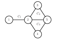
Figure 3: The graph with three cliques

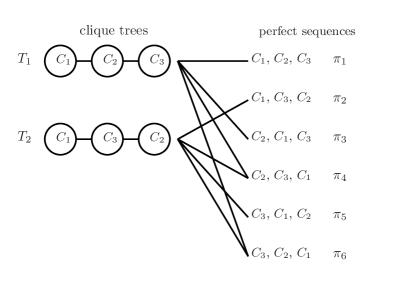
Figure 4: The bipartite graph of the clique trees and the perfect sequences for the graph in Figure 3

Now we consider to express this binary relations by the bipartite graph $B=({\cal T}\cup\varPi,{\cal R})$. We give a simple example. Figure 4 presents the bipartite graph $B$ for the graph in Figure 3. We see that $B$ is not complete.

In general Algorithm 4.1 does not necessarily generate every clique tree if an input perfect sequence is fixed. Conversely Algorithm 4.2 does not necessarily generate every perfect sequence if an input clique tree is fixed. Now we denote $\bar{\cal C}_{C}={\cal C}\setminus\{C\}$. Then the bipartite graph $B$ for the general chordal graph can be shown to have the following property.

Lemma 4.3.

Suppose that $C\in{\cal C}$ is simply separated. Let ${\cal T}_{\bar{\cal C}_{C}}\subset{\cal T}$ denote the set of clique trees for $G$ with an endpoint $C$. Then any two clique trees in ${\cal T}_{\bar{\cal C}_{C}}$ are connected on $B=({\cal T}\cup\varPi,{\cal R})$.

Proof..

We prove it by induction on the number $K=|{\cal C}|$ of the maximal cliques. If $K\leq 2$, the lemma is obvious. Suppose that $K\geq 3$ and that the lemma holds for all chordal graphs with fewer than $K$ maximal cliques.

Denote $G_{\bar{\cal C}_{C}}=G(V(\bar{\cal C}_{C}))$. First we note that ${\cal T}(G_{\bar{\cal C}_{C}})=\{T(\bar{\cal C}_{C})\mid T\in{\cal T}_{\bar{\cal C}_{C}}\}$ from Lemma 4.2. Since $C$ is simply separated, there exists a perfect sequence of $\bar{\cal C}_{C}$ from Theorem 3.3. Denote the set of such perfect sequences by $\varPi(\bar{\cal C}_{C})$. Let ${\cal R}(\bar{\cal C}_{C})\in{\cal T}(G_{\bar{\cal C}_{C}})\times\varPi(\bar{\cal C}_{C})$ be the symmetric binary relation in Definition 4.1 for $G_{\bar{\cal C}_{C}}$. Let $T$ and $T^{\prime}$ be any two clique trees in ${\cal T}_{\bar{\cal C}_{C}}$ and $T(\bar{\cal C}_{C})$ and $T^{\prime}(\bar{\cal C}_{C})$ be the subtree of $T$ and $T^{\prime}$ induced by $\bar{\cal C}_{C}$. From the inductive assumption, $T(\bar{\cal C}_{C})$ and $T^{\prime}(\bar{\cal C}_{C})$ are connected on the bipartite graph

$$B(\bar{\cal C}_{C})=\bigl{(}{\cal T}(G_{\bar{\cal C}_{C}})\cup\varPi(\bar{\cal C}_{C}),{\cal R}(\bar{\cal C}_{C})\bigr{)}.$$

Suppose that

$$T(\bar{\cal C}_{C})=\tilde{T}_{0},\tilde{\pi}_{1},\tilde{T}_{1},\dots,\tilde{T}_{p-1},\tilde{\pi}_{p},\tilde{T}_{p}=T^{\prime}(\bar{\cal C}_{C})$$

$$\tilde{T}_{i}=(\bar{\cal C}_{C},\tilde{{\cal E}}_{i})\in{\cal T}(G_{\bar{\cal C}_{C}}),\quad i=0,\dots,p,$$

$$\tilde{\pi}_{i}\in\varPi(\bar{\cal C}_{C}),\quad i=1,\dots,p$$

is a path from $T(\bar{\cal C}_{C})$ to $T^{\prime}(\bar{\cal C}_{C})$ on $B(\bar{\cal C}_{C})$. Since $C$ is simply separated, the sequence
$C_{\tilde{\pi}_{i}(1)},\dots,C_{\tilde{\pi}_{i}(K-1)},C$ is also a perfect sequence of $G$ for all $i=1,\dots,p$ from Corollary 3.1 and denote it by $\pi_{i}$. Let $C^{\prime}$ be the maximal clique which is adjacent to $C$ on $T^{\prime}$. Define $T_{i}$ by

$$T_{0}=T,\quad T_{i}=({\cal C},\tilde{{\cal E}}_{i}\cup\{(C,C^{\prime})\}),\quad i=1,\dots,p.$$

Since $(\tilde{T}_{i},\tilde{\pi}_{i})\in{\cal R}(\bar{\cal C}_{C})$ and $(\tilde{T}_{i-1},\tilde{\pi}_{i})\in{\cal R}(\bar{\cal C}_{C})$, we also have $(T_{i},\pi_{i})\in{\cal R}$ and $(T_{i-1},\pi_{i})\in{\cal R}$ from the definition of $T_{i}$. ∎

By using these lemmas we can show the connectivity of the bipartite graph $B$.

Theorem 4.1.

The bipartite graph $B=({\cal T}\cup\varPi,{\cal R})$ for any chordal graph $G$ is connected.

Proof..

For any perfect sequence $\pi$ there exists a clique tree $T$ such that $(T,\pi)\in{\cal R}$. Hence it suffices to show that any two clique trees are connected on $B$.

Let $T$ and $T^{\prime}$ be any two clique trees for $G$. Denote the set of endpoints in $T$ and $T^{\prime}$ by ${\cal L}(T)$ and ${\cal L}(T^{\prime})$, respectively. Suppose that $S$ is a minimal vertex separator which is minimal in ${\cal S}$ with respect to the inclusion relation. Let the connected components of $G({V}\setminus S)$ be denoted by $\Gamma_{1},\dots,\Gamma_{M}$. Then from Proposition 3.4 there exist maximal cliques $C_{a}\in{\cal L}(T)$, $C_{b}\in{\cal L}(T)$, $C_{a^{\prime}}\in{\cal L}(T^{\prime})$ and $C_{b^{\prime}}\in{\cal L}(T^{\prime})$ such that

$$C_{a}\setminus S\subseteq\Gamma_{a},\quad C_{b}\setminus S\subseteq\Gamma_{b},\quad a\neq b,$$

$$C_{a^{\prime}}\setminus S\subseteq\Gamma_{a^{\prime}},\quad C_{b^{\prime}}\setminus S\subseteq\Gamma_{b^{\prime}},\quad a^{\prime}\neq b^{\prime}$$

If the maximal cliques satisfy one of the following conditions,

$$C_{a}=C_{a^{\prime}},\quad C_{a}=C_{b^{\prime}},\quad C_{b}=C_{a^{\prime}},\quad C_{b}=C_{b^{\prime}},$$ (13)

then $T$ and $T^{\prime}$ are connected on $B$ from Lemma 4.3.

Suppose the maximal cliques do not satisfy any of the conditions in (13). Since $a^{\prime}\neq b^{\prime}$, one of $\Gamma_{a^{\prime}}$ and $\Gamma_{b^{\prime}}$ is not equal to $\Gamma_{a}$. We now assume $\Gamma_{a}\neq\Gamma_{b^{\prime}}$ without loss of generality. From Theorem 3.1 there exists a clique tree $T^{\prime\prime}$ such that both $C_{a}$ and $C_{b^{\prime}}$ are endpoints of it. Then from Lemma 4.3, $T$ and $T^{\prime\prime}$ are connected and $T^{\prime\prime}$ and $T^{\prime}$ are connected. Hence $T$ and $T^{\prime}$ are connected. ∎

5 Arbitrariness and uniqueness of the clique trees

In this section we consider to characterize chordal graphs from the aspect of the arbitrariness and the uniqueness of its clique trees. With respect to the arbitrariness of the clique trees, we can obtain the following result.

Theorem 5.1.

Let $G$ be a chordal graph with at least two maximal cliques. An arbitrary tree with the set of nodes ${\cal C}$ is a clique tree of $G$ if and only if $|{\cal S}|=1$.

Proof..

Suppose that $|{\cal S}|=1$ and $S\in{\cal S}$. Hence the only restriction imposed on the clique trees for $G$ is that ${\cal C}_{\uparrow S}$ induces a connected subtree. From (3) and (4), we have ${\cal C}_{\uparrow S}={\cal C}$. This implies that an arbitrary tree with the set of nodes ${\cal C}$ is a clique tree for $G$.

Conversely suppose that $|{\cal S}|\geq 2$. Let $S_{1}$ and $S_{2}$ be any two minimal vertex separators of $G$. Then ${\cal C}_{\uparrow S_{1}}\neq{\cal C}_{\uparrow S_{2}}$ from Lemma 2.5. Hence we can assume ${\cal C}_{\uparrow S_{2}}\setminus{\cal C}_{\uparrow S_{1}}\neq\emptyset$ without loss of generality and suppose $C\in{\cal C}_{\uparrow S_{2}}\setminus{\cal C}_{\uparrow S_{1}}$. Let $T^{\prime}$ be a clique tree such that the set of nodes is ${\cal C}_{\uparrow S_{1}}\cup\{C\}$ and $C\notin{\cal L}(T^{\prime})$. Then any clique tree $T$ such that $T^{\prime}=T({\cal C}_{\uparrow S_{1}}\cup\{C\})$ does not satisfy the condition that ${\cal C}_{\uparrow S_{1}}$ induces a connected subtree. ∎

On the other hand the necessary and sufficient condition for the clique tree to be unique is given as follows.

Theorem 5.2.

The clique tree for $G$ is unique if and only if

• $|{\cal S}|=|{\cal C}|-1$, i.e. $\nu(S)=1$ for all $S\in{\cal S}$;

• Any two minimal vertex separators of $G$ do not have the inclusion relation.

In order to prove Theorem 5.2, we note the following lemma.

Lemma 5.1.

${\cal S}$ satisfies the conditions (i) and (ii) in Theorem 5.2 if and only if $K_{S}=|{\cal C}_{\uparrow S}|=2$ for all $S$.

Proof..

Suppose that there exists $S\in{\cal S}$ satisfying $K_{S}\geq 3$. When $|{\cal S}({V}({\cal C}_{\uparrow S}))|\geq 2$, $S\subset S^{\prime}$ for all $S^{\prime}\neq S$, $S^{\prime}\in{\cal S}({V}({\cal C}_{\uparrow S}))$ from (iii) in Lemma 2.6. When $|{\cal S}({V}({\cal C}_{\uparrow S}))|=1$, $\nu(S)\geq 2$ from (ii) in Lemma 2.6. Hence ${\cal S}$ does not satisfy (i) or (ii).

Next we suppose that $|{\cal S}|<|{\cal C}|-1$. Then there exists $S\in{\cal S}$ such that $\nu(S)\geq 2$. From (3), $S$ satisfies $K_{S}\geq 3$.

Suppose that there exist $S\in{\cal S}$ and $S^{\prime}\in{\cal S}$ such that $S\subset S^{\prime}$. Then it is obvious that ${\cal C}_{\uparrow S}\supseteq{\cal C}_{\uparrow S^{\prime}}$. From Lemma 2.5, ${\cal C}_{\uparrow S}\neq{\cal C}_{\uparrow S^{\prime}}$. Hence ${\cal C}_{\uparrow S}\supset{\cal C}_{\uparrow S^{\prime}}$ and $K_{S}\geq 3$. ∎

Proof of Theorem 5.2. Let $T=({\cal C},{\cal E})$ be a clique tree for $G$. Suppose that ${\cal S}$ satisfies the conditions (i) and (ii). From Lemma 5.1, $K_{S}=2$ for all $S\in{\cal S}$. Hence the restriction that ${\cal C}_{\uparrow S}$ induces a connected subtree is equivalent to ${\cal C}_{\uparrow S}\in{\cal E}$, i.e. $\{{\cal C}_{\uparrow S}\mid S\in{\cal S}\}\subset{\cal E}$. The number of restrictions is

$$|{\cal S}|=K-1=|{\cal E}|.$$

Thus $\{{\cal C}_{\uparrow S}\mid S\in{\cal S}\}={\cal E}$. Hence $T$ is uniquely defined from the set of restrictions $\{{\cal C}_{\uparrow S}\mid S\in{\cal S}\}$.

Next we assume that $T$ is uniquely defined from $G$. Then it suffices to show that ${\cal S}$ satisfies (i) and (ii). We prove this by induction on the number of maximal cliques. When $K=2$, ${\cal S}$ satisfies $|{\cal S}|=1$. Hence ${\cal S}$ obviously satisfies (i) and (ii). Assume $K\geq 3$ and ${\cal S}$ satisfies (i) and (ii) for the chordal graphs with fewer than $K-1$ maximal cliques.

Let $C$ be an endpoint of $T$. From Theorem 3.1, there exists a perfect sequence $\pi\in\varPi$ such that $C_{\pi(K)}=C$. Denote $\bar{\cal C}_{C}={\cal C}\setminus\{C\}$ and $G_{\bar{\cal C}_{C}}=G(V(\bar{\cal C}_{C}))$. Define ${\cal T}(G_{\bar{\cal C}_{C}})$, $\varPi(\bar{\cal C}_{C})$ and ${\cal R}(\bar{\cal C}_{C})$ in the same way as in the proof of Lemma 4.3. Suppose that the clique trees for $G_{\bar{\cal C}_{C}}$ are not uniquely defined and let $\tilde{T}_{1}=(\bar{\cal C}_{C},{\cal E}_{1})$ and $\tilde{T}_{2}=(\bar{\cal C}_{C},{\cal E}_{2})$ be two clique trees in ${\cal T}(G_{\bar{\cal C}_{C}})$. Then there exist $\tilde{\pi}_{1}\in\varPi(\bar{\cal C}_{C})$ and $\tilde{\pi}_{2}\in\varPi(\bar{\cal C}_{C})$ satisfying

$$(\tilde{T}_{1},\tilde{\pi}_{1})\in{\cal R}(\bar{\cal C}_{C}),\quad(\tilde{T}_{2},\tilde{\pi}_{2})\in{\cal R}(\bar{\cal C}_{C}).$$

From Theorem 3.1, $C$ is simply separated, Hence both

$$C_{\tilde{\pi}_{1}(1)},\dots,C_{\tilde{\pi}_{1}(k-1)},C\quad\text{and}\quad C_{\tilde{\pi}_{2}(1)},\dots,C_{\tilde{\pi}_{2}(k-1)},C$$

are perfect sequences of ${\cal C}$ from Corollary 3.1 and denote them by $\pi_{1}$ and $\pi_{2}$, respectively. From Proposition 3.1 there exist $k_{1}<K$, $k_{2}<K$ and $S\in{\cal S}$ satisfying

$$C\cap\bigcup_{k=1}^{K-1}C_{\pi_{1}(k)}=C\cap C_{\pi_{1}(k_{1})}=S,\quad C\cap\bigcup_{k=1}^{K-1}C_{\pi_{2}(k)}=C\cap C_{\pi_{2}(k_{2})}=S.$$

Then

$$T_{1}=({\cal C},{\cal E}_{1}\cup(C,C_{\pi_{1}(k_{1})})),\quad T_{2}=({\cal C},{\cal E}_{2}\cup(C,C_{\pi_{2}(k_{2})})),$$

satisfy that $(T_{1},\pi_{1})\in{\cal R}$ and $(T_{2},\pi_{2})\in{\cal R}$ and that $T_{1}\neq T_{2}$. Hence both $T_{1}$ and $T_{2}$ are clique trees for $G$, which contradicts the assumption that $T$ is uniquely defined from $G$. Thus $|{\cal T}(\bar{\cal C}_{C})|=1$ and denote the unique tree by $\tilde{T}=(\bar{\cal C}_{C},\tilde{{\cal E}})$. Let $\tilde{\pi}\in\varPi(\bar{\cal C}_{C})$ be a perfect sequence satisfying $(\tilde{T},\tilde{\pi})\in{\cal R}(\bar{\cal C}_{C})$. Then $C_{\tilde{\pi}(1)},\dots,C_{\tilde{\pi}(K-1)},C$ is a perfect sequence of ${\cal C}$ from Corollary 3.1 and denote it by $\pi$.

From the inductive assumption ${\cal S}({V}(\bar{\cal C}_{C}))$ satisfies the conditions (i) and (ii). Suppose that there exists $S^{\prime}\in{\cal S}({V}(\bar{\cal C}_{C}))$ such that $S^{\prime}\supseteq S$. There exist at least two maximal cliques in $\bar{\cal C}_{C}$ which includes $S^{\prime}$. Denote two of such maximal cliques by $C_{1}$ and $C_{2}$. We note that $C\cap C_{1}=C\cap C_{2}=S$. Then both $T^{\prime}_{1}=({\cal C},\tilde{{\cal E}}\cup(C_{1},C))$ and $T^{\prime}_{2}=({\cal C},\tilde{{\cal E}}\cup(C_{2},C))$ satisfy $(T^{\prime}_{1},\pi)\in{\cal R}$ and $(T^{\prime}_{2},\pi)\in{\cal R}$, which contradicts the assumption. Hence there does not exist $S^{\prime}$ such that $S^{\prime}\supseteq S$.

Suppose that there exists $S^{\prime}\in{\cal S}({V}(\bar{\cal C}_{C}))$ such that $S^{\prime}\subset S$. Let $C^{\prime}$ be an endpoint of $T$ such that $C^{\prime}\neq C$. Then there exist $S^{\prime\prime}\in{\cal S}$ such that

$$C^{\prime}\cap V(\bar{\cal C}_{C^{\prime}})=S^{\prime\prime},$$

where $\bar{\cal C}_{C^{\prime}}={\cal C}\setminus\{C^{\prime}\}$. If $S^{\prime\prime}\subset S\in{\cal S}({V}(\bar{\cal C}_{C^{\prime}}))$, there exist at least two clique trees in $G$ by using the same argument as the above.

Consider the case where $S^{\prime\prime}\nsubseteq S$. Let $\tilde{T}^{\prime}=(\bar{\cal C}_{C^{\prime}},\tilde{{\cal E}}^{\prime})$ be the unique clique tree for $G(V(\bar{\cal C}_{C^{\prime}}))$. Then ${\cal S}({V}(\bar{\cal C}_{C^{\prime}}))$ satisfies the conditions (i) and (ii). We note that $S$, $S^{\prime}\in{\cal S}({V}(\bar{\cal C}_{C^{\prime}}))$. Since $S^{\prime}\subset S$, ${\cal C}_{\uparrow S^{\prime}}$ satisfies ${\cal C}_{\uparrow S^{\prime}}\subset{\cal C}_{\uparrow S}$. Hence $K_{S^{\prime}}\geq 3$, which contradicts the fact that $\tilde{T}^{\prime}$ is the unique clique tree for $G({V}(\bar{\cal C}_{C^{\prime}}))$ and ${\cal S}({V}(\bar{\cal C}_{C^{\prime}}))$ satisfies the conditions (i) and (ii). Hence there does not exist $S^{\prime}\in{\cal S}({V}(\bar{\cal C}_{C}))$ such that $S^{\prime}\subset S$. As a result ${\cal S}$ satisfies the conditions (i) and (ii). ∎

In the context of (2), we can obviously obtain the following result.

Theorem 5.3.

Define ${\cal M}_{S}$ and ${\cal C}_{\uparrow S}(\Gamma_{m}\cup S)$ as in (1). Then the conditions (i) and (ii) in Theorem 5.2 is equivalent to $|{\cal M}_{S}|=2$ and $|{\cal C}_{\uparrow S}(\Gamma_{m}\cup S)|=1$.

With respect to the uniqueness of the clique tree, we also obtain the following result.

Theorem 5.4.

Let $T$ be the unique clique tree defined from $G$. Then all maximal cliques which are simply separated are the endpoints of $T$.

Proof..

Suppose that $C$ is simply separated and that $C$ is not an endpoint of $T$. Then there exist at least two maximal cliques which are adjacent to $C$ on $T$. Denote them by $C_{1}$ and $C_{2}$. Note that $C\cap C_{1}\in{\cal S}$ and $C\cap C_{2}\in{\cal S}$. Denote $S_{1}=C\cap C_{1}$ and $S_{2}=C\cap C_{2}$. From Proposition 3.1 there exists $S\in{\cal S}$ satisfying (6) and hence $S_{1}$ and $S_{2}$ satisfy $S_{1}\subseteq S$ and $S_{2}\subseteq S$, respectively. $S_{1}=S$ and $S_{2}=S$ contradicts (i) in Theorem 5.2 and $S_{1}\subset S$ or $S_{2}\subset S$ contradicts (ii) in Theorem 5.2. ∎

6 Concluding remarks

In this article we considered characterizations of the set of clique trees in three ways. In Section 3 we addressed boundary cliques and gave some characterizations of endpoints of clique trees in relation to boundary cliques. In Section 4 we defined a symmetric binary relation between the set of clique trees and the set of perfect sequences of maximal cliques and we described the relation using a bipartite graph. We showed that the bipartite graph is connected for any chordal graphs. In Section 5 we derived a necessary and sufficient condition for the arbitrariness and for the uniqueness of their clique trees.

Theorem 4.1 and Theorem 5.2 are proved by induction on the number of maximal cliques. In the proof the notions of boundary cliques and the symmetric binary relation discussed in Section 4 are essential and the usefulness of them were confirmed.

Boundary cliques may be important from the algorithmic point of view. The detection of simply boundary cliques may contribute to more efficient generation of a perfect sequence of maximal cliques. The relation between boundary cliques and the simplicial partition used in a procedure of the isomorphism detection of chordal graphs in Nagoya[21] may be also interesting.

In Hara and Takemura [14], [15], we proposed statistical procedures whose performances depend on the choice of perfect sequences of maximal cliques for a given chordal graph. In this kind of situation it is desirable to optimize the performance over the set of perfect sequences. By the connectedness of the bipartite graph of Section 4 we can construct a connected Markov chain over the set of perfect sequences and search for the optimum perfect sequence.

By following Theorem 5.2, we see that the non-uniqueness of clique trees is related to the inclusion relations in ${\cal S}$ and the multiplicity of minimal vertex separators. This fact is important in enumerating all clique trees for a given chordal graph. By using this fact, we can provide another algorithm to enumerate all clique trees with the lists of maximal cliques and minimal vertex separators given as inputs.

We have obtained partial results on these problems. They are left for our future investigations.

Appendix

A Proof of Lemma 2.4

Proof of (i).  Denote $G_{m}=G(\Gamma_{m}\cup S)$. Suppose that there exists $m$ and $C\in{\cal C}(\Gamma_{m}\cup S)$ such that $C\cap\Gamma_{m}=\emptyset$, i.e. $C=S$. From the definition of the perfect sequence $S$ contains at least one minimal vertex separator $S^{\prime}\in{\cal S}(\Gamma_{m}\cup S)$ such that $S^{\prime}\subset S$. Then $S^{\prime}$ separates ${v}\in\Gamma_{m}$ and $S\setminus S^{\prime}$. Since $\Gamma_{m}\cap\Gamma_{m^{\prime}}=\emptyset$ for all $m^{\prime}\neq m$, $S^{\prime}$ also separates ${v}$ and any vertices in $\Gamma_{m^{\prime}}$, which contradicts the minimality of $S$ in ${\cal S}$ with respect to the inclusion relation. Hence $C\in{\cal C}(\Gamma_{m}\cup S)$ satisfies $C\cap\Gamma_{m}\neq\emptyset$ for all $m$. Choose ${v}_{m}\in C\cap\Gamma_{m}$.

Now suppose that there exists $C^{\prime}\in{\cal C}$ such that $C^{\prime}\supset C$ for $C\in{\cal C}(\Gamma_{m}\cup S)$. This implies that there exists $m^{\prime}\neq m$ such that $(C^{\prime}\setminus C)\cap\Gamma_{m^{\prime}}\neq\emptyset$. Choose ${v}_{m^{\prime}}\in(C^{\prime}\setminus C)\cap\Gamma_{m^{\prime}}$. Both ${v}_{m}$ and ${v}_{m^{\prime}}$ belong to $C^{\prime}$. However this contradicts the fact that $\Gamma_{m}$ and $\Gamma_{m^{\prime}}$ are not adjacent to each other for all $m^{\prime}\neq m$. Hence $\bigcup_{m=1}^{M}{\cal C}(\Gamma_{m}\cup S)\subseteq{\cal C}$.

Since $C\setminus S$ is connected for all $C\in{\cal C}$, there exists $m$ such that $C\subset\Gamma_{m}\cup S$. Noting that ${V}\supset\Gamma_{m}\cup S$, if $C$ is a maximal clique in $G$, then $C$ is also a maximal clique in $G_{m}$. Hence $\bigcup_{m=1}^{M}{\cal C}(\Gamma_{m}\cup S)\supseteq{\cal C}$. As a result we obtain $\bigcup_{m=1}^{M}{\cal C}(\Gamma_{m}\cup S)={\cal C}$.

Also it is easy to see that $\Gamma_{m}\cap\Gamma_{m^{\prime}}=\emptyset$ , $m\neq m^{\prime}$, implies ${\cal C}(\Gamma_{m}\cup S)\cap{\cal C}(\Gamma_{m^{\prime}}\cup S)=\emptyset$.

Proof of (ii).  Let $S^{\prime}$ be a minimal vertex separator in $G_{m}$. Then $G((\Gamma_{m}\cup S)\setminus S^{\prime})$ is disconnected. This implies that $G({V}\setminus S^{\prime})$ is also disconnected. Hence $S^{\prime}$ is a separator in $G$.

There exist ${v}\in\Gamma_{m}\cup S$ and ${v}^{\prime}\in\Gamma_{m}\cup S$ such that $S^{\prime}$ is the minimal ${v}-{v}^{\prime}$ separator in $G_{m}$. ${v}$ and ${v}^{\prime}$ are connected in $G((\Gamma_{m}\cup S)\setminus S^{\prime\prime})$ for $S^{\prime\prime}\subset S$. Since $G((\Gamma_{m}\cup S)\setminus S^{\prime\prime})$ is the induced subgraph of $G({V}\setminus S^{\prime\prime})$, ${v}$ and ${v}^{\prime}$ are also connected in $G({V}\setminus S^{\prime\prime})$. Hence $S^{\prime}$ is a minimal vertex separator of $G$. We have shown that ${\cal S}(\Gamma_{m}\cup S)\subseteq{\cal S}$. Now since $(\Gamma_{m}\cup S)\setminus S=\Gamma_{m}$ is connected, $S\notin{\cal S}(\Gamma_{m}\cup S)$. Hence ${\cal S}(\Gamma_{m}\cup S)$ is a proper subset of ${\cal S}$.

Proof of (iii).  It suffices to show it for $\Gamma_{1}$. Denote $K_{m}=|{\cal C}(\Gamma_{m}\cup S)|$. Let $\pi_{m}$ be a perfect sequence of ${\cal C}(\Gamma_{m}\cup S)$ such that $C_{\pi_{m}(1)}\supset S$. Let $S_{\pi_{m}(k)}\in{\cal S}(\Gamma_{m}\cup S)$, $k=2,\dots,K_{m}$ be the corresponding minimal vertex separator in $G_{m}$. Consider the sequence

$$C_{\pi_{1}(1)},\dots,C_{\pi_{1}(K_{1})},C_{\pi_{2}(1)},\dots,C_{\pi_{M}(K_{M})}.$$ (14)

Since $\Gamma_{m}\cap\Gamma_{m^{\prime}}=\emptyset$,

$$C_{\pi_{m}(1)}\cap\left(\bigcup_{m^{\prime}<m}\bigcup_{k^{\prime}\leq K_{m^{\prime}}}C_{\pi_{m^{\prime}}(k^{\prime})}\right)=(C_{\pi_{m}(1)}\cap S)\cup\left(C_{\pi_{m}(1)}\cap\bigcup_{m^{\prime}<m}\Gamma_{m^{\prime}}\right)=S\subset C_{\pi_{1}(1)}$$ (15)

and for $k^{\prime}\geq 2$

$$C_{\pi_{m}(k)}\cap\left(\bigcup_{m^{\prime}<m}\bigcup_{k^{\prime}\leq K_{m^{\prime}}}C_{\pi_{m^{\prime}}(k^{\prime})}\cup\bigcup_{k^{\prime}<k}C_{\pi_{m}(k^{\prime})}\right) =(C_{\pi_{m}(k)}\cap S)\cup\left(C_{\pi_{m}(k)}\cap\bigcup_{k^{\prime}<k}C_{\pi_{m}(k^{\prime})}\right)$$ (16)

$$=C_{\pi_{m}(k)}\cap\bigcup_{k^{\prime}<k}C_{\pi_{m}(k^{\prime})}.$$

Since $\pi_{m}$ is a perfect sequence of ${\cal C}(\Gamma_{m}\cup S)$, (i) of this lemma, (15) and (16) imply that (14) is a perfect sequence of ${\cal C}$.

Then there exists a clique tree such that the subgraph of it induced by ${\cal C}(\Gamma_{m}\cup S)$ is connected from Lemma 2.2. ∎

B List of notation

$G$	:	a connected chordal graph
$V$	:	the set of vertices in $G$
$G(V^{\prime})$	:	the subgraph of $G$ induced by $V^{\prime}\subset V$
${\cal C}$	:	the set of maximal cliques in $G$
${\cal C}(V^{\prime})$	:	the set of maximal cliques in $G(V^{\prime})$
$K$	:	the number of maximal cliques $|{\cal C}|$
$V({\cal C}^{\prime})$	:	$\displaystyle{\bigcup_{C\in{\cal C}^{\prime}}C}$ for ${\cal C}^{\prime}\subset{\cal C}$
${\cal S}$	:	the set of minimal vertex separators in $G$
${\cal S}(V^{\prime})$	:	the set of minimal vertex separators in $G(V^{\prime})$
$\nu(S)$	:	the multiplicity of $S\in{\cal S}$
${\cal T}$	:	the set of clique trees for $G$
${\cal T}(G(V^{\prime}))$	:	the set of clique trees for $G(V^{\prime})$
$T({\cal C}^{\prime})$	:	the subtree of $T\in{\cal T}$ induced by ${\cal C}^{\prime}\subset{\cal C}$
$\varPi$	:	the set of perfect sequences of ${\cal C}$
$\varPi({\cal C}^{\prime})$	:	the set of perfect sequences of ${\cal C}^{\prime}$
$G_{{\cal C}^{\prime}}$	:	$G(V({\cal C}^{\prime}))$	Sec 4, 5
$V_{m,m^{\prime}}$	:	$V({\cal C}\setminus\{C_{m},C_{m^{\prime}}\})$, $C_{m}$, $C_{m^{\prime}}\in{\cal C}$	Prop. 3.4
${\cal C}_{\uparrow S}$	:	$\{C\in{\cal C}\mid C\supset S,S\in{\cal S}\}$	Sec 2, 5
$\bar{{\cal C}}_{C}$	:	${\cal C}\setminus\{C\}$	Sec 4, 5
$N_{G}(v)$	:	the open adjacency set of $v\in V$ in $G$	Sec 2, 3
$N_{G}[v]$	:	the closed adjacency set of $v\in V$ in $G$	Sec 3
$N_{G}(V^{\prime})$	:	$\displaystyle{\bigcup_{v\in V^{\prime}}N_{G}(v)\setminus V^{\prime}}$	Sec 3
$N_{G}[V^{\prime}]$	:	$\displaystyle{\bigcup_{v\in V^{\prime}}N_{G}[v]}$	Sec 3
$\Gamma_{1},\dots,\Gamma_{M}$	:	the connected components of $G(V\setminus S)$	Sec 2, 3, 4
$G_{m}$	:	$G(\Gamma_{m}\cup S)$	Appendix A
${\cal M}_{S}$	:	$\{m\mid N_{G}(\Gamma_{m})=S\}$	(1), (2), Th. 5.3
${\cal C}_{\uparrow S}(\Gamma_{m}\cup S)$	:	$\{C\in{\cal C}\mid C\subseteq\Gamma_{m}\cup S,C\supset S\}$	(1), (2), Th. 5.3
$K_{S}$	:	$|{\cal C}_{\uparrow S}|$	Lemma 2.6
$K_{m}$	:	$|{\cal C}(\Gamma_{m}\cup S)|$	Appendix A
$\mathrm{Simp}(C)$	:	the simplicial component in $C\in{\cal C}$	Sec 2, 3
$\mathrm{Sep}(C)$	:	the non-simplicial component in $C\in{\cal C}$	Sec 2, 3
${\cal T}_{{\cal C}^{\prime}}$	:	$\{T\in{\cal T}\mid T({\cal C}^{\prime})\text{ is connected}\}$	Lemma 4.2, 4.3
${\cal L}(T)$	:	the set of endpoints in $T\in{\cal T}$	Prop. 3.4, Th. 4.1
${\cal C}_{\pi(k)}$	:	$\{C_{\pi(1)},\dots,C_{\pi(k)}\}$ for $\pi\in\varPi$	Th. 2.2, Lemma 3.1
${\cal R}$	:	the symmetric binary relation on ${\cal T}\times\varPi$	Def. 4.1, Sec. 4, 5
${\cal R}({\cal C}^{\prime})$	:	the symmetric binary relation on ${\cal T}(G_{{\cal C}^{\prime}})\times\varPi({\cal C}^{\prime})$	Sec. 4, 5

References

- [1] Agnarsson, G. and Halldórsson M. M.(2004). On coloring of squares of outerplanar graphs, Proceedings of the Fifteenth Annual ACM-SIAM Symposium on Discrete Algorithms, New Orleans, LA, 237-246.
- [2] Bernstein, P. A. and Goodman, N.(1981). Power of natural semijoins, SIAM J. Comput., 10, 751-771.
- [3] Booth, K. S. and Johnson, J. H.(1982). Dominating sets in chordal graphs, SIAM J. Comput., 11, 191-199.
- [4] Buneman, P. (1974). A characterization on rigid circuit graphs, Discrete Math., 9, 205-212.
- [5] Chang, M. S. and Peng, S. L.(1992). A simple linear time algorithm for the domatic partition problem on strongly chordal graphs, Inform. Process. Lett., 43, 297-300.
- [6] Dirac, G. A. (1961). On rigid circuit graphs, Abhandlungen Mathematisches Seminar Hamburg, 25, 71-76.
- [7] Dobra, A. (2003). Markov bases for decomposable graphical models, Bernoulli, 9, 1093-1108.
- [8] Fukuda, M., Kojima, M., Murota, K. and Nakata, K. (2000). Exploiting sparsity in semidefinite programming via matrix completion. I. General framework. SIAM J. Optim., 11, 647–674.
- [9] Farber, M.(1983). Characterization of strongly chordal graphs, Discrete Mathematics, 43, 173-189.
- [10] Gavril, F.(1974). The intersection graphs of subtrees in trees are exactly the chordal graphs, J. Combin. Theory Ser. B, 116, 47-56.
- [11] Geiger, D., Meek C. and Sturmfels. B. (2006). On the toric algebra of graphical models. To appear in Annals of Statistics.
- [12] Golumbic, M. C.(1980). Algorithmic Graph Theory and Perfect Graphs, Academic Press, New York.
- [13] Grone, C. R., Johnson, C. R., Sá E. M. and Wolkowicz, H.(1984). Positive definite completions of partial Hermitian matrices, Linear Algebra Appl., 58, 109-124.
- [14] Hara, H. and Takemura, A.(2005a). Improving on the maximum likelihood estimators of the means in Poisson decomposable graphical models, Technical Reports, METR, 2005-08, Department of Mathematical Informatics, University of Tokyo. To appear in J. Multivariate Anal.
- [15] Hara, H. and Takemura, A.(2005b). Bayes Admissible Estimation of the Means in Poisson Decomposable Graphical Models, Technical Report, METR, 2005-22, Department of Mathematical Informatics, University of Tokyo, 2005. Submitted for publication.
- [16] Ho, C. W. and Lee, R. C. T.(1989). Counting clique trees and computing perfect elimination schemes in parallel, Inform. Process. Lett., 31, 61-68.
- [17] Jensen, F. V.(1996). An Introduction to Bayesian Networks, UCL Press, London.
- [18] Kumar, P. S. and Madhavan C. E. V.(2002). Clique tree generalization and new subclasses of chordal graphs, Discrete. Appl. Math., 117, 109-131.
- [19] Kumar, P. S. and Prasad, N. K. R.(1998). On generating strong elimination orderings of strongly chordal graphs, Foundations of Software Technology and Theoretical Computer Science (Chennai), Lecture Notes in Computer Science, LNCS-1530, 221-232.
- [20] Lauritzen, S. L.(1996). Graphical Models, Clarendon Press, Oxford.
- [21] Nagoya, T.(2001). Counting Graph Isomorphisms among Chordal Graphs with Restricted Clique Number, In Proceeding of 12th International Symposium on Algorithms and Computation, ISAAC 2001, Christchurch, New Zealand, LNCS Vol. 2223, 136-147.
- [22] Rose, D. J.(1970). Triangulated graphs and the elimination process, J. Math. Anal. Appl., 32, 597-609.
- [23] Shibata, Y.(1988). On the tree representation of chordal graphs, J. Graph Theory, 12, 421-428.
- [24] Tarjan, R. E. and Yannakakis, M.(1984). Simple linear-time algorithm to test chordality of graphs, test acyclicity of hypergraphs and selectively reduce acyclic hypergraph. SIAM J. Comput., 13, 565-579.
- [25] Waki, H., Kim, S., Kojima, M. and Muramatsu, M. (2006). Sums of squares and semidefinite program relaxations for polynomial optimization problems with structures sparsity. SIAM J. Optim., 17, 218–242.
- [26] Whittaker, J.(1990). Graphical Models in Applied Multivariate Statistics, John Wiley & Sons, Chichester.