INSTITUT NATIONAL DE RECHERCHE EN INFORMATIQUE ET EN AUTOMATIQUE

Interactive Hatching and Stippling by Example
Pascal Barla — Simon Breslav — Lee Markosian — Joëlle Thollot N° 6461
Juin 2006

Abstract: We describe a system that lets a designer interactively draw patterns of strokes in the picture plane, then guide the synthesis of similar patterns over new picture regions. Synthesis is based on an initial user-assisted analysis phase in which the system recognizes distinct types of strokes (hatching and stippling) and organizes them according to perceptual grouping criteria. The synthesized strokes are produced by combining properties (e.g., length, orientation, parallelism, proximity) of the stroke groups extracted from the input examples. We illustrate our technique with a drawing application that allows the control of attributes and scale-dependent reproduction of the synthesized patterns.

Key-words: Expressive rendering, NPR

Hachurage et pointillage par l’exemple

Résumé : Ce rapport présente une méthode permettant à un artiste de dessiner interactivement un motif 2D de hachures ou de points puis de guider la synthèse d’un motif similaire. La synthèse s’appuie sur une phase d’analyse assistée par l’utilisateur dans laquelle le système extrait et organise des points ou des hachures (segments) selon des critères de regroupement perceptuel. La synthèse est alors effectuée en combinant les propriétés (longueur, orientation, parallélisme, proximité) des éléments extraits par l’analyse.

Mots-clés : Rendu expressif

1 Introduction

1.1 Motivation

An important challenge facing researchers in non-photorealistic rendering (NPR) is to develop hands-on tools that give artists direct control over the stylized rendering applied to drawings or 3D scenes. An additional challenge is to augment direct control with a degree of automation, to relieve the artist of the burden of stylizing every element of complex scenes. This is especially true for scenes that incorporate significant repetition within the stylized elements. While many methods have been developed to achieve such automation algorithmically outside of NPR (e.g., procedural textures), these kind of techniques are not appropriate for many NPR styles where the stylization, directly input by the artist, is not easily translated into an algorithmic representation. An important open problem in NPR research is thus to develop methods to analyze and synthesize artists’ interactive input.

In this work, we focus on the synthesis of stroke patterns that represent tone and/or texture. This particular class of drawing primitives have been investigated in the past (e.g., [SABS94, WS94, Ost99, DHvOS00, DOM⁺01]), but with the goal of accurately representing tone and/or texture coming from a photograph or a drawing. Instead, we orient our research towards the faithful reproduction of the expressiveness, or style, of an example drawn by the user, and to this end analyze the most common stroke patterns found in illustration, comics or traditional animation: hatching and stippling patterns.

Our goal is thus to synthesize stroke patterns that ”look like” an example pattern input by the artist, and since the only available evaluation method of such a process is visual inspection, we need to give some insights into the perceptual phenomena arising from the observation of a hatching or stippling pattern. In the early 20th century, Gestalt psychologists came up with a theory of how the human visual system structures pictorial information. They showed that the visual system first extracts atomic elements (e.g., lines, points, and curves), and then structures them according to various perceptual grouping criteria like proximity, parallelism, continuation, symmetry, similarity of color, velocity, etc. This body of research has grown consequently under the name of perceptual organization (see for example the proceedings of POCV, the IEEE Workshop on Perceptual Organization in Computer Vision). We believe it is of particular importance when studying artists’ inputs.

1.2 Related work

The idea of synthesizing textures, both for 2D images and 3D surfaces, has been extensively addressed in recent years (e.g. by Efros and Leung [EL99], Turk [Tur01], and Wei and Levoy [WL01]). Note, however, that this body of research is concerned with painting and synthesizing textures that are represented as images. In contrast, we are concerned with direct painting and synthesis of stroke patterns represented in vector form. I.e., the stroke geometry is represented explicitly as connected vertices with attributes such as width and color. While this vector representation is typically less efficient to render, it has the important advantage that strokes can be controlled procedurally to adapt to changes in the depicted regions (strokes can vary in opacity, thickness and/or density to depict an underlying tone.)

Stroke pattern synthesis systems have been studied in the past, for example to generate stipple drawings [DHvOS00], pen and ink representations [SABS94, WS94], engravings [Ost99], or for painterly rendering [Her98]. However, they have relied primarily on generative rules, either chosen by the authors or borrowed from traditional drawing techniques. We are more interested in analysing reference patterns drawn by the user and synthesizing new ones with similar perceptual properties.

Kalnins et al. [KMM⁺02] described an algorithm for synthesizing stroke “offsets” (deviations from an underlying smooth path) to generate new strokes with a similar appearance to those in a given example set. Hertzmann et al. [HOCS02], as well as Freeman et al. [FTP03] address a similar problem. Neither method reproduces the inter-relation of strokes within a pattern. Jodoin et al. [JEGPO02] focus on synthesizing hatching strokes, which is a relatively simple case in which strokes are arranged in a linear order along a path. The more general problem of reproducing organized patterns of strokes has remained an open problem.

1.3 Overview

In this paper, we present a new approach to analyze and synthesize hatching and stippling patterns in 1D and 2D. Our method relies on user-assisted analysis and synthesis techniques that can be governed by different behaviors. In every case, we maintain low-level perceptual properties between the reference and synthesized patterns and provide algorithms that execute at interactive rates to allow the user to intuitively guide the synthesis process.

The rest of the paper is organized as follows. We describe the analysis phase in Section 2, and the synthesis algorithm and associated “behaviors” in Section 3. We present results in Section 4, and conclude in Section 5 with a discussion of our method and possible future directions.

2 Analysis

We structure a stroke pattern according to perceptual organization principles: a pattern is a collection of groups (hatching or stippling); a group is a distribution of elements (points or lines); and an element is a cluster of strokes. For instance, the user can draw a pattern like the one in Figure 1, which is composed of sketched line segments, sometimes with a single stroke, sometimes with multiple overlapping strokes; our system then clusters the strokes in line elements that hold specific properties; and finally structures the elements into a hatching group that holds its own properties. We restrict our analysis to homogeneous groups with an approximate uniform distribution of their elements: hatching groups are made only of lines, stippling groups made only of points. This approach could be extended to more complex elements, using the clustering technique of Barla et al. [BTS05].

Figure 1: A simple example of the analysis process in 1D: the strokes input by the user (top) are analyzed to extract elements (bottom, in light gray), that are further organized along a path (dashed polyline).

As a general rule of thumb, we consider that involving the user in the analysis gives him or her more control over the final result, at the same time removing complex ambiguities. Thus, in our system, the user first specifies the high-level properties of the stroke pattern he is going to describe. He chooses a type of pattern (hatching or stippling); this determines the type of elements to be analyzed (lines for hatching, points for stippling). He then chooses a 1D or 2D reference frame within which the elements will be placed. He finally sets the scale $\epsilon$ of the elements, measured in pixels: intuitively, $\epsilon$ represents the maximum diameter of analysed points, and the maximum thickness of analyzed lines.

Once these parameters are set, the user draws strokes as polyline gestures. Depending on the group type, points or lines at the scale $\epsilon$ are extracted and structured: Then statistics about perceptual properties of the strokes are computed. This whole processus has an instant feedback, so that the user can vary $\epsilon$ and observe changes made to the analysis in real-time. We first describe how elements are extracted given a chosen $\epsilon$ and their analyzed properties; then we describe how those elements are structured into a group, and how perceptual measures that characterize this group are extracted.

2.1 Element analysis

The purpose of element analysis is to cluster a set of strokes drawn by the user into points or lines, depending on the chosen element type. To this end, we use a greedy algorithm that processes strokes in the drawing order, and tries to cluster them until no more clustering can be done. We first fit each input stroke to an element (point or line) at the scale $\epsilon$. Strokes that cannot be fit to an element are flaged invalid and will be ignored in the remaining steps of the analysis. Then, valid pairs of elements that can be perceived as a single element are clustered iteratively. The fitting and clustering of points and lines is illustrated in Figure 2.

For points, the fitting is performed by computing the center of gravity $c$ of a stroke $S$ and measuring its spread $s_{p}=2\max_{p\in S}|p-c|$. If $s_{p}>\epsilon$, then the stroke is flaged invalid because the circle of center $c$ and diameter $s_{p}$ do not encloses $S$. The clustering of two points is made by computing the center of gravity $c^{*}$ of the points and measuring its spread $s_{p}^{*}$. Similarly, if $s_{p}^{*}>\epsilon$, then the points cannot be clustered. This allows the system to recognize any cluster of short strokes relative to the scale $\epsilon$, like point clusters, small circled shapes, crosses, etc. (See Section 4.)

For lines, the fitting is performed by computing the virtual line $l_{v}$ of a stroke $S$ and measuring its spread $s_{l}=2\max(d_{H}(S,l_{v}),d_{H}(l_{v},S))$ where $d_{H}(X,Y)=\max_{x\in X}(\min_{y\in Y}|x-y|)$ is the Hausdorff distance between two sets of points. The virtual line can be computed by least-square fitting, but in practice we found that using the endpoint line is enough and faster. Then, if $s_{l}>\epsilon$, the stroke is flaged invalid because the line segment of axis $l_{v}$ and thickness $s_{l}$ do not enclose $S$. The clustering of two lines is made by computing the virtual line $l_{v}^{*}$ of the lines and measuring its spread $s_{l}^{*}$. The virtual line can be computed by least-square fitting on the whole set of points; but we preferred to apply least-square fitting only on the two endpoints of each clustered line for efficiency reasons. Then, if $s_{l}^{*}>\epsilon$, the lines cannot be clustered. This allows the system to recognize any set of strokes that resembles a line segment at the scale $\epsilon$. Examples including sketched lines, overlapping lines, and dashed lines are shown in Section 4.

Once points or lines have been extracted, we can compute their properties: extent, position and orientation. The extent property represents the dimensions of the element: point size or line length and width. For point size, we use the spread of the element. For lines, we use the length of the virtual line and its spread (for width). Orientation represents the angle between a line and the reference frame main direction (the main axis for 1D frames, the X-axis for the cartesian frame). It is always ignored for points. We add a special position property for 1D reference frames: since they are synthesized in 2D (in the picture plane), 1D patterns have a remaining degree of freedom that is represented by the position of elements perpendicular to the main axis. For all these properties, we compute statistics (a mean and a standard deviation) and boundary values (a min and a max); We also store the gesture input by the user and will refer to it as the shape of the element in the rest of the paper.

Figure 2: Top left: A stroke is fit to a point. Bottom left: A pair of points is clustered into a new point. Top right: A stroke is fit to a line. Bottom right: A pair of lines is clustered into a new line.

2.2 Group analysis

A group is considered to be an approximately uniform distribution of elements within a reference frame. This means that while analyzing a reference group, we are not interested in the exact distribution of its elements: we consider a reference group as a small sample of a bigger, approximately uniform distribution of the same elements. Consequently, we first need to extract a local structure that describes the neighborhood of each element; this local structure will then be reproduced more or less uniformly throughout the pattern during synthesis.

To this end, we begin with the computation of a graph that structures the elements locally: in 1D, we build a chain that orders strokes along the main axis; whereas in 2D, we compute a Delaunay triangulation. We only keep the edges that: (a) connect two valid elements and (b) connect an element to its nearest neighbor. We chose this because the synthesis algorithm (described in Section 3) converges only when considering nearest neighbor edges. However, this decision is also justified from a perceptual point of view: basing our analysis on nearest neighbors emphasizes the proximity property of element pairs, which is known to be a fundamental perceptual organization criterion.

For each edge of the resulting graph, we extract the following perceptual properties, taking inspiration from Etemadi et al. [ESM⁺91]: proximity for points and lines; parallelism, overlapping and separation for lines only.

[0,r,,] Proximity is simply taken to be the euclidean distance between the centers of the two elements in pixels. We not only compute this measure for points, but also for lines in order to initialize our synthesis algorithm (see Section 3.) Let’s note $\Delta$ the vector from one point to the other, then we have

$$prox=||\Lambda||$$ (1)

with $prox\in[0,+\infty)$.

[0,r,,] To compute parallelism, we first find the accute angle made between the two lines. Since there is no apriori order on the line pair, we take the absolute value of this accute angle and normalize it between $0$ and $1$. Let’s note $\Theta$ the accute angle, then we compute parallelism using

$$par=|\frac{2\Theta}{\pi}|$$ (2)

with $par\in[0,1]$.

[0,r,,] Like Etemaldi et al. [ESM⁺91], we define overlapping relative to the bissector of the considered line pair. But we modify slightly their measure to meet our needs: We project the center of each line on the bissector and use them to define an overlapping vector $\Delta$. Overlapping is computed using the following formula:

$$ov=\frac{2||\Delta||}{L_{1}^{*}+L_{2}^{*}}$$ (3)

where $L_{1}^{*}$ and $L_{2}^{*}$ are the lengths of the lines projected on the bissector. Note that with this definition, $ov=0$ means a perfect overlapping.

[0,r,,] Finally, separation represents the distance between two lines, this time in the direction perpendicular to their bissector. We project the center of each line on a line perpendicular to the bissector and use them to define a separation vector $\Gamma$. Separation is then computed with the following formula:

$$sep=||\Gamma||$$ (4)

with $sep\in[0,+\infty)$.

We compute statistics (a mean and a standard deviation) and bounds (a min and a max) for each of these properties.

3 Synthesis

The purpose of the synthesis process is to create a new stroke pattern that has the same properties (for elements and groups) as the reference pattern. We first describe a general algorithm that is able to create a new pattern meeting this objective; then we show how to customize it through the use of synthesis behaviors.

3.1 Algorithm

Our synthesis algorithm can be summarized as follows:

1. Build a graph where the edge lengths follow the proximity statistics;

2. Synthesize an element at each graph node using element properties;

3. Correct elements position and orientation using element pair properties.

The first step is achieved using Lloyd relaxation [Llo82]. This technique starts with a random distribution of points in 1D or 2D. It then computes the Voronoi diagram of the set of points, and moves each point to the center of its Voronoi region. When applied iteratively, the algorithm converges to an even distribution of points. Deussen et al. [DHvOS00] observed that the variance of nearest neighbor edge length decreases with each iteration. We use this to get a variance (in nearest neighbor edge length) that approximately matches that of the reference pattern.

Consider the mean $\mu^{*}$, standard deviation $\sigma^{*}$, and the ratio $r^{*}=\sigma^{*}/\mu^{*}$ of a given property in our reference pattern. We start with a random point set by distributing $N=N_{ref}\mathcal{A}/\mathcal{A}_{ref}$ points, where $N_{ref}$ is the number of elements in the reference pattern, and $\mathcal{A}_{ref}$ and $\mathcal{A}$ are the area of the reference and target patterns, respectively. We then apply the Lloyd technique, computing $\mu$, $\sigma$ and $r=\sigma/\mu$ of the current distribution at each step until $r<r^{*}$. Note that $\mu$ will have changed throughout the set of iterations. Thus, in order to have $\mu=\mu^{*}$, we finally rescale the distribution by $\mu^{*}/\mu$. An example of Lloyd’s method is shown in Figure 3.

In the second step, for each node of the graph we first pick a reference element $E$. Then we choose a set of element properties and compute a position, orientation and scale for $E$. There are many different approaches to choose element properties; the ones we implemented are detailed in the next section, and for now we only present the general algorithm.

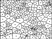
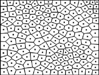
(a)	(b)

Figure 3: (a) An input random distribution and its Voronoi diagram. (b) The result after iteratively applying Lloyd’s method until a desired variance-to-mean ratio in edge length is obtained.

We first position the center of $E$ at its corresponding node location. In the case of a 1D reference frame, we also move $E$ perpendicularly to the main axis using the relative position property. Then, $E$ is scaled using the extent property; however, we impose a constraint on scaling for each type of element. In order for points to remain points, we ensure that their size is smaller than $\epsilon$; and similarly for lines, we ensure that their width is no more than $\epsilon$. Finally, $E$ is rotated based on orientation. For a 1D reference frame, we rotate $E$ so that the angle with the local X-axis matches the orientation property. For a 2D reference frame, we use the angle with the global X-axis instead.

Finally, in the third step, for each node of the graph, we compute a corrected set of parameters that takes into account the perceptual properties of nearest neighbor pairs extracted from the reference pattern during analysis. We use a greedy algorithm where each node is corrected toward its nearest neighbor in turn. In order to get a consistent correction, we add two procedures to this algorithm: first, the nodes are sorted according to the proximity with their nearest neighbor in a preprocess, so that the perceptually closest elements are corrected in priority; second, when a node is corrected, we discard both nodes of its edge from upcoming corrections, in order to ensure that the current correction stays valid throughout the algorithm.

We now describe how an element is corrected based on perceptual measures. In a way similar to what we did for element properties, we choose a set of perceptual properties for element pairs. The details of how we perform this choice are explained in the next section. Note that the correction is not directly applied to the initial set of parameters: the user can control through linear interpolation the amount of correction he or she wishes to apply.

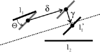
(a)	(b)

Figure 4: (a) A point is corrected by displacing it along the direction to its nearest neighbor to match a proximity measure. (b) A line is first rotated to match parallelism, then displaced along and perpendicularly to the bissector direction to match overlapping and separation.

For points, the only parameter to correct is position: we simply move the selected point along the line through its nearest neighbor to match the desired proximity (see Figure 4(a).) Let’s consider $prox_{1}$ and $prox_{2}$, the current and desired proximity values respectively. Then the correction applied to the position of current point is given by the following translation vector:

$$\lambda_{prox_{1}\rightarrow prox_{2}}=\frac{\Lambda_{1}}{||\Lambda_{1}||}.(prox_{2}-prox_{1})$$ (5)

If we are dealing with lines, we first correct the orientation of the current element based on the parallelism property we want to enforce; then we correct its position using overlapping and separation (see Figure 4(a).) The reason why we first correct the orientation is that the overlapping property is highly dependent on the parallelism of lines.

Let’s consider $par_{1}$ and $par_{2}$, the current and desired parallelism values respectivelly. Then the correction applied to the orientation of current point is given by the following angle:

$$\theta_{par_{1}\rightarrow par_{2}}=sign(\Theta_{1}).(par_{2}-par_{1}).\frac{\pi}{2}$$ (6)

Finally, we correct lines using a combination of overlapping and separation. For two overlapping values $ov_{1}$ and $ov_{2}$ for the current and target position, we translate the current line along the bissector line using the following vector:

$$\delta_{ov_{1}\rightarrow ov_{2}}=\frac{\Delta_{1}}{||\Delta_{1}||}.(ov_{2}-ov_{1}).\frac{(L_{1}^{*}+L_{2}^{*})}{2}$$ (7)

Then we translate it perpendicularly to the bissector using:

$$\gamma_{sep_{1}\rightarrow sep_{2}}=\frac{-\Gamma_{1}}{||\Gamma_{1}||}.(sep_{2}-sep_{1})$$ (8)

Note that the last two operations do not change the parallelism property.

3.2 Behaviors

We now present the synthesis behaviors that are responsible for assigning a value for each property. We developed several behaviors because we believe that the ability to synthesize patterns that are more or less close to the reference pattern is a desirable feature: it lets us balance fidelity and variation relative to the reference pattern.

We thus implemented three behaviors: sampling, copying and cloning, that range from close to the statistical distribution to close to the reference data. In the same spirit, we let the user choose the amount of correction that is applied. The correction results are displayed interactively. We now turn to the description of the three behaviors.

Sampling

This behavior produces patterns whose properties exhibit the same statistics as those of the reference pattern. For each property, we compute the mean and standard deviation of values in the input pattern to derive a Gaussian distribution function, then sample its inverse cumulative function to yield values that follow the distribution of the reference pattern. If the sampled value lies outside the range of values in the reference pattern, the sampling is repeated until a value in the original range of values is produced. The reference element whose shape is to be copied is then randomly chosen.

Copying

Moving toward increased fidelity to the reference pattern, this behavior assigns each property independently by copying values from randomly chosen elements in the reference pattern. For pairs, the reference pair with most similar value is found, and the synthesized pair is altered to match the reference pair. As an example, consider the proximity property of element pairs. If a nearest-neighbor pair of synthesized elements is separated by $n$ pixels, we first find the reference pair whose proximity $m$ is closest to $n$. We then correct the position of the chosen synthesized element to achieve a proximity of $m$ pixels. For element shape, we first pick the reference pair with the most similiar proximity value and copy one of its element randomly.

Cloning

The cloning behavior synthesizes patterns that most closely follow the reference pattern. It is a modification of the copy behavior where all the properties are taken from the same source. Given a synthesized element, we randomly choose a reference element and copy all its properties to the synthesized element. Pairs are handled similarly, but the choice is not random: during correction, in order to stay close to the statistical distribution produced by Lloyd’s method, we first find the reference pair with the most similar proximity property, then adjust parameters of the chosen synthesized element to yield the same pair-wise properties. The element shape is chosen like with the copying behavior.

4 Results

Figure 5(a)-(d) shows reference and synthesized hatching and stippling groups in 1D and 2D. For these examples, we used the copying behavior and chose the correction amount manually. Note that complex elements extracted in the analysis phase are reproduced during synthesis: crosses and small circles for stippling, sketched strokes and multiple overlapping lines for hatching. The relations among nearest-neighbor synthesized elements are replicated from corresponding reference elements. Figure 5(e) shows a limitation of our method: the synthesis fails to reproduce recognizable stroke sequences seen in the input pattern. This is due to the small neighborhood size (only nearest neighbor) used in synthesis. The computation times are interactive, up to a couple of seconds for the most complex patterns we synthesized.

We compare our different behaviors in Figure 5(f)-(g), using two reference 1D hatching patterns. With a quasi-uniform pattern (similar orientation, spacing, etc.), the sampling behavior has the advantage of synthesizing patterns with more variation, creating strokes in positions and orientations that were not present in the reference pattern, whereas the cloning behavior reproduces strokes and nearest neightbor relations found in the reference pattern. With a more irregular reference pattern, the sampling behavior produces patterns that lack the broader coherence of the example pattern, while the cloning behavior synthesizes patterns with more fidelity. Although not shown here, the copying behavior produces intermediate results, providing a trade-off between fidelity and variation.

To illustrate our synthesis technique, we developed a 2D drawing application that lets the user draw example hatching or stippling patterns, then guide the synthesis of similar patterns over selected image regions. The system can vary stroke attributes such as color, thickness and opacity according to colors or tones in a provided background image (see Figure 6, left). This lets us create colored strokes that represent shadows, highlights and intermediate tones. The final illustration is composed of the synthesized patterns, optionally composited on top of the background image. The system can also synthesize multiple versions of the same pattern at different resolutions, supporting the scale-dependent reproductions of the output image, for simple levels-of-detail or for printing purpose (see Figure 6, right).

(a)
(b)
(c)
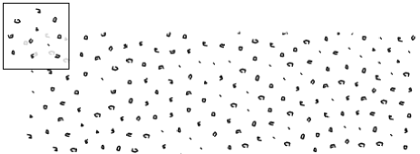
(d)
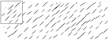
(e)
(f)
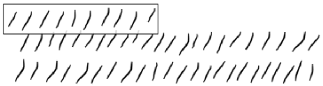
(g)

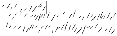
Figure 5: (a)-(d) Stippling and hatching results in 1D and 2D with their reference pattern (small boxes); (e) A synthesis failure example; (f) For uniform patterns, sampling (top) introduces more variation than cloning (bottom); (g) For less uniform patterns, sampling (top) is more incoherent than cloning (bottom).

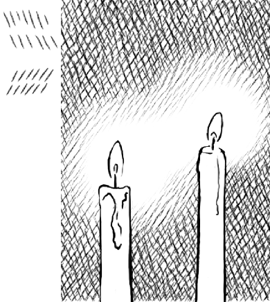
Figure 6: Two examples from our drawing application. Left: the thickness of the lines is controled by a user-defined mask; Right: levels-of-detail of a drawing (bottom) are automatically synthesized from an initial resolution (top).

5 Discussion and future work

The main limitation of our approach is that we only consider nearest neighbor relations. To our knowledge, the first and only attempt to deal with larger neighborhoods is the work of Jodoin et al. [JEGPO02]. However, they only consider parametric elements of the same dimension, organized along a 1D path with no perceptual analysis (though they acknowledge the importance of extracting low-level perceptual properties). On the other hand, our approach is a step in another direction: we consider more general elements thanks to our element analysis, and introduce low-level perceptual properties in our group analysis. We also generalize the synthesis to 2D patterns. These two approaches are not incompatible, however. We look forward to combining advantages of both methods to develop a more general solution to the example-based stroke pattern synthesis problem.

We believe that extending our method to bigger neighborhoods, exploiting perceptual properties for neighborhood comparisons, is the logical next step towards this solution. It is interesting to compare our method to work done on texture synthesis on surfaces (e.g., Turk [Tur01] and Wei and Levoy [WL01]). In those systems and ours, the first step is to build a lattice that models the correspondence between the input (2D texture or reference stroke pattern) and the output (a 2D surface or target distribution of elements). The second step initializes nodes of the lattice with values that follow the statistics of the reference pattern or texture. In the final step, node values are modified based on neighborhood comparisons of various sizes, either at random [WL01] or in a predefined order (line sweeping in [Tur01], nearest neighbors in our work). This observation opens promising avenues for building on the existing body of texture synthesis techniques.

For our clustering algorithm, we relied on the drawing order, but we might investigate other orderings, for instance based on proximity. This would even be mandatory in cases where the reference pattern is extracted from an image and the drawing order is not known. We also considered only points and lines and the perceptual relations among them. However, other primitives like arcs or more complex curves have been studied from a perceptual organization point of view, and we plan to incorporate them in our system in future work. Other perceptual criteria like symmetry or closeness might then be of great value for those patterns. Finally, even if we believe that a user-assisted analysis is the most valuable approach, one might consider automating the process for specific applications (e.g. for capturing the style of an existing drawing). This implies determining the group type, reference frame and $\epsilon$ automatically.

6 Conclusions

We presented a new approach to stroke synthesis by example, for two particular classes of patterns: hatching and stippling (in 1D and 2D). Our method is fast and easy to implement. Its interactive response and its different synthesis behaviors let the user guide the synthesis process. The resulting synthesized patterns are perceptually similar to the reference ones, but also add a degree of variation. This lets us use our tool in a drawing application, with features such as stroke attribute control for efficient image depiction, and scale-dependent synthesis for levels-of-detail.

References

- [BTS05] Pascal Barla, Joëlle Thollot, and François Sillion. Geometric clustering for line drawing simplification. In Proceedings of the Eurographics Symp. on Rendering, 2005.
- [DHvOS00] Oliver Deussen, Stefan Hiller, Cornelius van Overveld, and Thomas Strothotte. Floating points: A method for computing stipple drawings. Computer Graphics Forum, 19(3), 2000.
- [DOM+01] Frédo Durand, Victor Ostromoukhov, Mathieu Miller, Francois Duranleau, and Julie Dorsey. Decoupling strokes and high-level attributes for interactive traditional drawing. In Rendering Techniques 2001: 12th Eurographics Workshop on Rendering, pages 71–82, 2001.
- [EL99] Alexei A. Efros and Thomas K. Leung. Texture synthesis by non-parametric sampling. In IEEE International Conference on Computer Vision, pages 1033–1038, 1999.
- [ESM+91] A. Etemadi, J.P. Schmidt, G. Matas, J. Illingworth, and J.V. Kittler. Low-level grouping of straight line segments. In British Machine Vision Conf., pages 119–126, 1991.
- [FTP03] William T. Freeman, Joshua B. Tenenbaum, and Egon C. Pasztor. Learning style translation for the lines of a drawing. ACM Trans. Graph., 22(1):33–46, 2003.
- [Her98] Aaron Hertzmann. Painterly rendering with curved brush strokes of multiple sizes. In Proceedings of SIGGRAPH 98, pages 453–460, 1998.
- [HOCS02] Aaron Hertzmann, Nuria Oliver, Brian Curless, and Steven M. Seitz. Curve analogies. In Rendering Techniques 2002: 13th Eurographics Workshop on Rendering, pages 233–246, June 2002.
- [JEGPO02] Pierre-Marc Jodoin, Emric Epstein, Martin Granger-Piché, and Victor Ostromoukhov. Hatching by example: a statistical approach. In Proceedings of NPAR 2002, pages 29–36, 2002.
- [KMM+02] Robert D. Kalnins, Lee Markosian, Barbara J. Meier, Michael A. Kowalski, Joseph C. Lee, Philip L. Davidson, Matthew Webb, John F. Hughes, and Adam Finkelstein. WYSIWYG NPR: Drawing strokes directly on 3D models. ACM Trans. on Graphics, 21(3):755–762, July 2002.
- [Llo82] S. P. Lloyd. Least squares quantization in pcm. IEEE Trans. on Information Theory, 28(2):129–137, 1982.
- [Ost99] Victor Ostromoukhov. Digital facial engraving. In Proceedings of SIGGRAPH 99, pages 417–424, 1999.
- [SABS94] Michael P. Salisbury, Sean E. Anderson, Ronen Barzel, and David H. Salesin. Interactive pen-and-ink illustration. In Proceedings of SIGGRAPH 94, pages 101–108, 1994.
- [Tur01] Greg Turk. Texture synthesis on surfaces. In Proceedings of ACM SIGGRAPH 2001, pages 347–354, 2001.
- [WL01] Li-Yi Wei and Marc Levoy. Texture synthesis over arbitrary manifold surfaces. In Proceedings of ACM SIGGRAPH 2001, pages 355–360, 2001.
- [WS94] Georges Winkenbach and David H. Salesin. Computer-generated pen-and-ink illustration. In Proceedings of SIGGRAPH 94, pages 91–100, 1994.