Methods for Partitioning Data to Improve Parallel Execution Time for Sorting on Heterogeneous Clusters

Abstract

The aim of the paper is to introduce general techniques in order to optimize the parallel execution time of sorting on a distributed architectures with processors of various speeds. Such an application requires a partitioning step. For uniformly related processors (processors speeds are related by a constant factor), we develop a constant time technique for mastering processor load and execution time in an heterogeneous environment and also a technique to deal with unknown cost functions. For non uniformly related processors, we use a technique based on dynamic programming. Most of the time, the solutions are in ${\cal O}(p)$ ($p$ is the number of processors), independent of the problem size $n$. Consequently, there is a small overhead regarding the problem we deal with but it is inherently limited by the knowing of time complexity of the portion of code following the partitioning.
Keywords: parallel in-core sorting, heterogeneous computing, complexity of parallel algorithms, data distribution.

The advent of parallel processing, in particular in the context of cluster computing is of particular interest with the available technology. A special class of non homogeneous clusters is under concern in the paper. We mean clusters whose global performances are correlated by a multiplicative factor. We depict a cluster by the mean of a vector set by the relative speeds of each processor.

In this paper we develop general techniques in order to control the execution time and the load balancing of each node for applications running in such environment. What is important over the application we consider here, is the meta-partitioning schema which is the key of success. All the approaches we develop can be considered as static methods: we predetermine the size of data that we have to exchange between processors in order to guarantee that all the processors end at the same time before we start the execution. So, this work can be considered in the domain of placement of tasks in an heterogeneous environment.

Many works have been done in data partitioning on heterogeneous platforms, among them Lastovetsky’s and Reddy’s work [1] that introduces a scheme for data partitioning when memory hierarchies from one CPU to another are different. There, the heterogeneity notion is related to the heterogeneity of the memory structure. Under the model, the speed of each processor is represented by a function of the size of the problem. The authors solve the problem of partitioning $n$ elements over $p$ heterogeneous processors in ${\cal O}(p^{2}\times\log_{2}n)$ time complexity.

Drozdowski and Lawenda in [2] propose two algorithms that gear the load chunk sizes to different communication and computation speeds of applications under the principle of divisible loads (computations which can be divided into parts of arbitrary sizes; for instance painting with black pixels a whole image). The problem is formalized as a linear problem solved either by branch and bound technique or a genetic algorithm. Despite the fact that the architecture is large enough (authors consider heterogeneous CPU and heterogeneous links), we can not apply it here because our problem cannot be expressed under the framework of ’divisible loads’: in our case, we need to merge sorted chunks after the partitioning step and the cost is not a linear one…thus our new technique.

The organization of our paper is the following. In section 1 we introduce the problem of sorting in order to characterize the difficulties of partitioning data in an heterogeneous environment. The section motivates the work. In section 2 we recall our previous techniques and results. Section 3 is devoted to a new constant time solution and deals also with unknown cost functions. In section 4 we introduce a dynamic programming approach and we recall a technique that do not assume a model of processors related by constant integers but in this case the processor speed may be “unrelated”. Section 5 is about experiments and section 6 concludes the paper.

1 Target applications and implementation on heterogeneous clusters

Assume that you have a set of $p$ processors with different speeds, interconnected by a crossbar. Initially, the data is distributed across the $p$ processors and according to the speeds: the slowest processor has less data than the quickest. This assumption describes the initial condition of the problem. In this section we detail our sorting application for which performance are directly related to this initial partitioning.

1.1 Parallel Sort.

Efficient parallel sorting on clusters (see [3, 4, 5, 6, 7, 8] for the homogeneous case and [9, 10, 11, 12, 13] for the heterogeneous case) can be implemented in the following ways:

1. Each processor sorts locally its portion and picks up representative values in the sorted list. It sends the representative values to a dedicated node.

2. This node sorts what it receives from the processors and it keeps $p-1$ pivots; it distributes the pivots to all the processors.

3. Each processor partitions its sorted input according to the pivots and it sends $p-1$ portions to the others.

4. Each processor merges what it received from the others.

Note that the sorting in step 1 can be bypassed but in this case the last step is a sort not a merge. Moreover note that there is only one communication step: the representative values can be selected by sampling few candidates at a cost much lower than the exchange of values. In other words, when a value moves, it goes to the final destination node in one step.

2 Previous results and parallel execution time

Consider the simple problem of local sorting, such as presented in [10] (and our previous comments). The sizes $n_{i}$ of data chunks on each node is assumed to be proportional to the speed of processors.

Let us now examine the impact on the parallel execution time of sorting of the initial distribution or, more precisely, the impact of the redistribution of data. We determine the impact in terms of the way of restructuring the code of the meta partitioning scheme that we have introduced above. In the previous section, when we had $N$ data to sort on $p$ processors depicted by their respective speeds $k1,\cdots,k_{p}$, we had needed to distribute to processor $p_{i}$ an amount $n_{i}$ of data such that:

$$n_{1}/k_{1}=n_{2}/k_{2}=.....=n_{p}/k_{p}$$ (1)

and

$$n_{1}+n_{2}+....+n_{p}=N$$ (2)

The solution is:

$$\forall i,n_{i}=N\times k_{i}/(k_{1}+k_{2}+...+k_{p})$$

Now, since the sequential sorts are executed on $n_{i}$ data at a cost proportional $n_{i}\ln n_{i}$ time cost (approximatively since there is a constant in front of this term), there is no reason that the nodes terminate at the same time since $n_{1}/k_{1}\ln n_{1}\neq n_{2}/k_{2}\ln n_{2}\neq\cdots\neq n_{p}/k_{p}\ln n_{p}$ in this case. The main idea that we have developed in [14] is to send to each processor an amount of data to be treated by the sequential sorts proportional to $n_{i}\ln n_{i}$. The goal is to minimize the global computation time $T=\min(\max_{i=1,\ldots,p}n_{i}\ln n_{i})$ under the constraints $\sum n_{i}=N$ and $n_{i}\geq 0$.

It is straightforward to see that an optimal solution is obtained if the computation time is the same for all processors (if a processor ends its computation before another one, it could have been assigned more work thus shortening the computation time of the busiest processor). The problem becomes to compute the data sizes $n^{\prime}_{1},\cdots,n^{\prime}_{p}$ such that:

$$n^{\prime}_{1}+n^{\prime}_{2}+\cdots+n^{\prime}_{p}=N$$ (3)

and such that

$$(n^{\prime}_{1}/k_{1})\ln n^{\prime}_{1}=(n^{\prime}_{2}/k_{2})\ln n^{\prime}_{2}=\cdots=(n_{p}^{\prime}/k_{p})\ln n^{\prime}_{p}$$ (4)

We have shown that this new distribution converges to the initial distribution when $N$ tends to infinity. We have also proved in [14] that a constant time solution based on Taylor developments leads to the following solution:

$$n_{i}=\frac{k_{i}}{K}N+\epsilon_{i},\ \ \ (1\leq i\leq p)\ \mbox{where}\ \epsilon_{i}=\frac{N}{\ln N}\left[\frac{k_{i}}{K^{2}}\sum_{j=1}^{p}k_{j}\ln\left(\frac{k_{j}}{k_{i}}\right)\right]$$ (5)

and where $K$ is simply the sum of the $k_{i}$. These equations give the sizes that we must have to install initially on each processors to guaranty that the processors will terminate at the same time. The time cost of computing one $k_{i}$ is ${\cal O}(p)$ and is independent of $n$ which is an adequate property for the implementations since $p$ is much lower and not of the same order than $n$.

One limitation of above the technique is that we assume that the cost time of the code following the partitioning step should admit a Taylor development. We introduce now a more general approach to solve the problem of partitioning data in an heterogeneous context. It is the central part of the work. We consider an analytic description of the partitioning when the processors are uniformly related: processor $i$ has an intrinsic relative speed $k_{i}$.

3 General exact analytic approach on uniformly related processors

The problem we solved in past sections is to distribute batches of size $N$ according to (4). We will first replace the execution time of the sorting function by a generic term $f(n)$ (which would be $f(n)=n\ln n$ for a sorting function, but could also be $f(n)=n^{2}$ for other sorting algorithms, or any function corresponding to different algorithms). We assume that $f$ is a strictly increasing monotonous integer function. We can with this consider a more general approach to task distribution in parallel algorithms. Since our processors have an intrinsic relative speed $k_{i}$, the computation time of a task of size $n_{i}$ will be $f(n_{i})/k_{i}$. This (discrete) function can be extended to a (real) function $\tilde{f}$ by interpolation. We can try to solve this equation exactly through analytical computation. We define the common execution time $T$ through the following equation:

$$T=\frac{\tilde{f}(n_{1})}{k_{1}}=\frac{\tilde{f}(n_{2})}{k_{2}}=\cdots=\frac{\tilde{f}(n_{p})}{k_{p}}$$ (6)

and equation

$$n_{1}+n_{2}+....+n_{p}=N$$ (7)

Let us recall that monotonous increasing functions can have an inverse function. Therefore, for all $i$, we have $\tilde{f}(n_{i})=Tk_{i}$, and thus:

$$n_{i}=\tilde{f}^{-1}(Tk_{i})$$ (8)

Therefore, we can rewrite (7) as:

$$\sum_{i=1}^{p}\tilde{f}^{-1}(Tk_{i})=N$$ (9)

If we take our initial problem, we have only one unknown term in this equation which is $T$. The sum $\sum_{i=1}^{p}\tilde{f}^{-1}(Tk_{i})$ is a strictly increasing function of $T$. If we suppose $N$ large enough, there is a unique solution for $T$. The condition of $N$ being large enough is not a rough constraint. $\tilde{f}^{-1}(T)$ is the number of data that can be treated in time $T$ by a processor speed equals to $1$. If we consider that $\tilde{f}^{-1}(0)=0$ (which is reasonable enough), we obtain that $\sum_{i=1}^{p}\tilde{f}^{-1}(Tk_{i})=0$ for $T=0$.

Having $T$, it is easy to compute all the values of $n_{i}=\tilde{f}^{-1}(Tk_{i})$. We shall show later on how this can be used in several contexts. Note also that the computed values have to be rounded to fit in the integer numbers. If the numbers are rounded down, at most $p$ elements will be left unassigned to a processor. The processors will therefore receive a batch of size $n_{i}=\left\lfloor\tilde{f}^{-1}(Tk_{i})\right\rfloor+\tilde{\delta_{i}}$ to process. $\delta_{i}$ can be computed with the following (greedy) algorithm:

1. Compute initial affectations $\tilde{n}_{i}=\left\lfloor\tilde{f}^{-1}(Tk_{i})\right\rfloor$ and set $\delta_{i}=0$;

2. For each unassigned item of the batch of size $N$ (at most $p$ elements) do:

   1. Choose $i$ such that $(\tilde{n}_{i}+\delta_{i}+1)/k_{i}$ is the smallest;

   2. Set $\delta_{i}=\delta_{i}+1$.

The running time of this algorithm is $O(p\log p)$ at most, so independant of the size of the data $N$.

3.1 Multiplicative cost functions

Let us consider now yet another cost function. $f$ is a multiplicative function if it verifies $f(xy)=f(x)f(y)$. If $f$ is multiplicative and admits an inverse function $g$, its inverse is also multiplicative:

$$g(ab)=g(f(g(a))f(g(b)))=g(f(g(a)g(b)))=g(a)g(b)$$

If $\tilde{f}$ is such a function (e.g. $f(n)=n^{k}$), we can solve equation (9) as follows:

$$N=\sum_{i=1}^{p}\tilde{f}^{-1}(Tk_{i})=\sum_{i=1}^{p}\tilde{f}^{-1}(T)\tilde{f}^{-1}(k_{i})=\tilde{f}^{-1}(T)\sum_{i=1}^{p}\tilde{f}^{-1}(k_{i})$$ (10)

We can then extract the value of $T$:

$$\tilde{f}^{-1}(T)=\frac{N}{\sum_{i=1}^{p}\tilde{f}^{-1}(k_{i})}$$ (11)

Combining it with (8) we obtain:

$$n_{i}=\tilde{f}^{-1}(Tk_{i})=\tilde{f}^{-1}(T)\tilde{f}^{-1}(k_{i})=\frac{\tilde{f}^{-1}(k_{i})}{\sum_{i=1}^{p}\tilde{f}^{-1}(k_{i})}N$$ (12)

Hence the following result:

Theorem 3.1

If $f$ is a cost function with the multiplicative property $f(ab)=f(a)f(b)$, then the size of the assigned sets is proportional to the size of the global batch with a coefficient that depends on the relative speed of the processor $k_{i}$:

$$n_{i}=\frac{\tilde{f}^{-1}(k_{i})}{\sum_{i=1}^{p}\tilde{f}^{-1}(k_{i})}N$$

This results is compatible with the usual method for linear functions (split according to the relative speeds), and gives a nice generalization of the formula.

3.2 Sorting: the polylogarithmic function case

Many algorithms have cost functions that are not multiplicative. This is the case for the cost $\Theta(n\log n)$ of the previous sequential part of our sorting algorithm, and more generally for polylogarithmic functions. However, in this case equation 9 can be solved numerically. Simple results show that polylogarithmic functions do not yield a proportionality constant independent of $N$.

3.2.1 Mathematical resolution for the case $n\ln n$

In the case $f(n)=n\ln n$, the inverse function can be computed. It makes use of the Lambert W function $W(x)$, defined as being the inverse function of $xe^{x}$. The inverse of $f:n\mapsto n\ln n$ is therefore $g:x\mapsto x/W(x)$.

The function $W(x)$ can be approached by well-known formulas, including the ones given in [15]. A development to the second order of the formula yields $W(x)=\ln x-\ln\ln(x)+o(1)$, and also:

$$\frac{x}{W(x)}=\frac{x}{\ln(x)}\frac{1}{1-(\ln\ln(x)/\ln(x))+o(1)}=\frac{x}{\ln(x)}\left(1+{\frac{\ln\ln(x)}{\ln(x)}}+{\mathcal{O}}\left(\left({\frac{\ln\ln(x)}{\ln(x)}}\right)^{2}\right)\right)$$

This approximation leads us to the following first-order approximation that can be used to numerically compute in ${\mathcal{O}}(p)$ the value of $T$:

Theorem 3.2

Initial values of $n_{i}$ can be asymptotically computed by

$$\sum_{i=1}^{p}\frac{Tk_{i}+Tk_{i}\ln\ln(Tk_{i})}{(\ln(Tk_{i}))^{2}}=N\text{ and }n_{i}=\frac{Tk_{i}+Tk_{i}\ln\ln(Tk_{i})}{(\ln(Tk_{i}))^{2}}$$

3.3 Unknown cost functions

Our previous method also claims an approach to unknown cost functions. The general outline of the method is laid out, but needs refinement according to the specific needs of the software platform. When dealing with unknown cost functions, we assume no former knowledge of the local sorting algorithm, just linear speed adjustments (the collection of $k_{i}$). We assume however that the algorithm has a cost function, i.e. a monotonous increasing function of the size of the data $C$. Several batch of data are submitted to our software. Our method builds an incremental model of the cost function. At first, data is given in chunks of size proportionnal to each node’s $k_{i}$. The computation time on node $i$ has a duration of $T_{n_{i}}$ and thus a basic complexity of $C(n_{i})=T_{n_{i}}k_{i}$. We can thus build a piecewise affine function (or more complex interpolated function, if heuristics require that) that represents the current knowledge of the system about the time cost $n\mapsto C(n)$. Other values will be computed by interpolation. The list of all known points can be sorted, to compute $f$ efficiently.

The following algorithm is executed for each task:

1. For each node $i$, precompute the mapping $(T,i)\mapsto n_{i}$ as previously, using interpolated values for $f$ if necessary (see below). Deduce a mapping $T\mapsto n$ by summing the mappings over all $i$.

2. Use a dichotomic search through $T\mapsto n$ mapping to find the ideal value of $T$ (and thus of all the $n_{i}$) and assign chunks of data to node $i$;

3. When chunk $i$ of size $n_{i}$ is being treated:

   1. Record the cost $C=T_{n_{i}}k_{i}$ of the computation for size $n_{i}$.

   2. If $n_{i}$ already had a non-interpolated value, choose a new value $C^{\prime}$ according to whatever strategy it fits for the precise platform and desired effect (e.g. mean value weighted by the occurrences of the various $C$ found for $n_{i}$, mean value weighted by the complexity of the itemset, max value). Some strategies may require storing more informations than just the mapping $n\mapsto C(n)$.

   3. If $n_{i}$ was not a known point, set $C^{\prime}=C$.

   4. Ensure that the mapping as defined by $n\neq n_{i}\mapsto C(n)$ and the new value $n_{i}\mapsto C^{\prime}$ is still monotonous increasing. If not, raise or lower values of neighboring known points (this is simple enough to do if the strategy is to represent the cost with a piecewise function). Various heuristics can be applied, such as using the weighted mean value of conflicting points for both points.

4. At this point, the precomputation of the mappings will yield consistent results for the dichotomic search. A new batch can begin.

The initial extrapolation needs care. An idea of the infinite behavior of the cost function toward infinity is a plus. In absence of any idea, the assumption that the cost is linear can be a starting point (a “linear guess”). All “linear guesses” will yield chunks of data of the same size (as in equation (4)). Once at least one point has been computed, the “linear guess” should use a ratio based on the complexity for the largest chunk size ever treated (e.g. if size $1,000$ yields a cost of $10,000$, the linear ratio should be at least $10$).

4 A dynamic programming technique for non-uniformly related processors

In the previous sections we have developed new constant time solution to estimate the amount of data that each processor should have in its local memory in order to ensure that the parallel sorts end at the same time. The complexity of the method is the same than the complexity of the method introduced in [14].

The class of functions that can be used according to the new method introduced in the paper is large enough to be useful in practical cases. In [14], the class of functions captured by the method is the class of functions that admit a Taylor development. It could be a limitation of the use of the two methods.

Moreover, the approach of [14] considers that the processor speeds are uniformly related, i.e. proportional to a given constant. This is a restriction in the framework of heterogeneous computers since the time to perform a computation on a given processor depends not only on the clock frequency but also on various complex factors (memory hierarchy, coprocessors for some operations).

In this section we provide a general method that provides an optimal partitioning $n_{i}$ in the more general case. This method is based on dynamic programming strategy similar to the one used in FFTW to find the optimal split factor to compute the FFT of a vector [16].

Let us give some details of the dynamic approach. Let $f_{i}(m)$ be the computational cost of a problem of size $m$ on machine $i$. Note that two distinct machines may implement different algorithms (e.g. quicksort or radix sort) or even the same generic algorithm but with specific threshold (e.g. Musser sort algorithm with processor specific algorithm to switch from quicksort to merge sort and insertion sort). Also, in the sequel the $f_{i}$ are not assumed proportional.

Given $N$, an optimal partitioning $(n_{1},\ldots,n_{p})$ with $\sum_{i=1}^{p}n_{i}=N$ is defined as one that minimizes the parallel computation time $T(N,p)$;

$$T(N,p)=\max\{{\vtop{\hbox{\hfill$f_{i}(n_{i});\hfill$}\hbox{\raise 2.0pt\hbox{$\scriptstyle i=1,\ldots,p$}}}}\}=\min_{(x_{1},\ldots,x_{p})\in\mathbb{N}^{p}:\sum_{i=1}^{p}x_{i}=N}\max\{{\vtop{\hbox{\hfill$f_{i}(x_{i});\hfill$}\hbox{\raise 2.0pt\hbox{$\scriptstyle i=1,\ldots,p$}}}}\}$$

A dynamic programming approach leads to the following inductive characterization of the solution:$\forall(m,i)\mbox{~{}with~{}}0\leq m\leq N\mbox{~{}and~{}}1\leq i\leq p:T(m,i)=\min_{n_{i}=0..m}\max(f_{i}(n_{i}),C(m-n_{i},i-1))$

Then, the computation of the optimal time $T(N,p)$ and of a related partition $(n_{i})_{i=1,\ldots,p}$ is obtained iteratively in ${\cal O}(N^{2}.p)$ time and ${\cal O}(N.p)$ memory space.

The main advantage of the method is that it makes no assumption on the functions $f_{i}$ that are non uniformly related in the general case. Yet, the potential drawback is the computational overhead for computing the $n_{i}$ which may be larger than the cost of the parallel computation itself since $T(N,p)=o(N^{2}p)$. However, it can be noticed, as in [16], that this overhead can be amortized if various input data are used with a same size $N$. Moreover, some values $T(m,p)$ for $m\leq K$ may be precomputed and stored. Than in this case, the overhead decreases to $O\left(p.\left(\frac{N}{K}\right)^{2}\right)$. Sampling few values for each $n_{i}$ enables to reduce the overhead as desired, at the price of a loss of optimality.

5 Experiments

We have conducted experiments on the Grid-Explorer platform in order to compare our approach for partitioning with partitioning based only on the relative speeds. Grid-Explorer is a project devoted to build a large scale experimental grid. The Grid-Explorer platform is connected also to the nation wide project Grid5000 which is the largest Grid project in France. We consider here only the Grid-Explorer platform which is built with bi-Opteron processors (2Ghz, model 246), 80GB of IDE disks (one per node). The interconnection network is made of Cisco switches allowing a bandwidth of 1Gb/s full-duplex between any two nodes. Currently, the Grid-Explorer platform has 216 computation nodes (432 CPU) and 32 network nodes (used for network emulation - not usefull in our case). So, the platform is an homogeneous platform.

For emulating heterogeneous CPU, two techniques can be used. One can use the CPUfreq driver available with Linux kernels (2.6 and above) and if the processor supports it; the other one is CPU burning. In this case, a thread with high priority is started on each node and consumes Mhz while another process is started for the main program. In our case, since we have bi-opteron processors we have chosen to run 2 processes per node and doing CPU burning, letting Linux to run them one per CPU. Feedback and experience running the CPUfreq driver on a bi-processor node, if it exists, is not frequent. This explain why we use the CPU burning technique.

Figure 1 shows the methodology of running experiments on the Grid-Explorer or Grid5000 platforms. Experimenters take care of deploying codes and reserve nodes. After that, they configure an environment (select specific packages and a Linux kernel, install them) and reboot the nodes according to the environment. The experiments take place only after installing this “software stack” and at a cost which is significant in term of time.

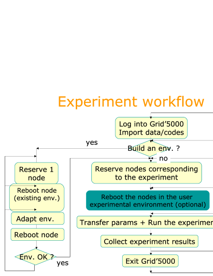
Figure 1: Methodology of experiments on the Grid-Explorer platform

We have implemented the sorting algorithm depicted in subsection 1.1 and according to Theorem 3.2 for the computation of the initial amount of data on each node for minimizing the total execution time. Note that each node generates its local portion on the local disk first, then we start to measure the time. It includes the time for reading from disk, the time to select and to exchange the pivots, the time for partitioning data according to the pivots, the time for redistributing (in memory) the partitions, the time for sorting and finally the time to write the result on the local disks.

We sort records and each record is 100 bytes long. The first 10 bytes is a random key of 10 printable characters. We are compliant with the requirements of Minute Sort as much as possible in order to beat the record in a couple of weeks.

We proceed with 50 runs per experiment. We only consider here experiments with a ratio of 1.5 between processor speeds. This is a strong constraint: the more the ratio is high the more the difference in execution time is important and in favor of our algorithm. So we have two classes of processor but the choice between the performance ($1$ or $1/1.5$) is made at random. We set half of the processors with a performance of $1$ and the remainder with a performance of $1/1.5$. We recall that the emulation technique is ’CPU burning’.

Since we have observed that the communication time has a significant impact on the total execution time, we have developed two strategies and among them, one for using the second processor of the nodes. In the first implementation communication take place in a single thread that is to say in the thread also doing computation. In the second implementation we have created a thread for sending and a thread for receiving the partitions. We guess that the operating system allocates them on the ’second’ processor of our bi-opteron cards equiped with a single Gigabit card for communication.

The input size is 541623000 records (54GB) because it provides about an execution time of one minute in the case of an homogeneous run using the entire 2Ghz. Note that it corresponds approximatively to 47% of the size of the 2005 Minute Sort record.

We run 3 experiments. Only experiments A.2 et A.3 use our technique to partition the data whereas experiment A.1 corresponds to a partitioning according to the relative speed only. In other words, experiment A.1 corresponds to the case where the CPU burns X.Mhz (where X is either 1Ghz or 1/1.5 GHz) but the performance vector is set according to an homogeneous cluster, we mean without using our method for re-balancing the work. Experiment A.2 also corresponds to the case where communication are not done in separate threads (and thus they are done on the same processor). Experiment A.3 corresponds to the case where the CPU burns X Mhz (also with X is either 1Ghz or 1/1.5 GHz) and communication are done in separate threads (and thus they are done on separate processors among the two available on a node). We use the pthread library and LAM-MPI 7.1.1 which is a safe-thread implementation of MPI.

A1 experiment	A2 experiment	A3 experiment
125.4s	112.7s	69.4s

Figure 2: Summary of experiments

sorting 54GB on 96 nodes is depicted in Figure 2. We observe that the multithreaded code (A.3) for implementating the communication step is more efficient than the code using a single thread (A.2). This observation confirms that the utilization of the second processor is benefit for the execution time. Concerning the data partitioning strategy introduced in the paper, we observe a benefit of about 10% in using it (A.2) comparing to A.1. Moreover, A.3 and A.2 use the same partitioning step but they differ in the communication step. The typical cost of the communication step is about 33% of the execution time for A.3 and about 60% for A.2.

6 Conclusion

In this paper we address the problem of data partitioning in heterogeneous environments when relative speeds of processors are related by constant integers. We have introduced the sorting problem in order to exhibit inherent difficulties of the general problem.

We have proposed new ${\cal O}(p)$ solutions for a large class of time complexity functions. We have also mentioned how dynamic programming can find solutions in the case where cost functions are “unrelated” (we cannot depict the cpu performance by the mean of integers) and we have reminded a recent and promising result of Lastovetsky and Reddy related to a geometrical interpretation of the solution. We have also described methods to deal with unknown cost functions. Experiments based on heteroneous processors correlated by a factor of 1.5 and on a cluster of 96 nodes (192 AMD Opteron 246) show better performance with our technique compared to the case where processors are supposed to be homogeneous. The performance of our algorithm is even better if we consider higher factor for the heterogeneity notion, demonstrating the validity of our approach.

In any case, communication costs are not yet taken into account. It is an important challenge but the effort in modeling seems important. In fact you cannot mix, for instance, information before the partitioning with information after the partitioning in the same equation. Moreover, communications are difficult to precisely modelize in a complex grid archtitecture, where various network layers are involved (Internet/ADSL, high speed networks,…). In this context, a perspective is to adapt the static partitioning, such as proposed in this paper, by a dynamic on-line redistribution of some parts of the pre-allocated chunks in reaction to network overloads and resources idleness (e.g. distributed work stealing).

References

- [1] Lastovetsky, A., Reddy, R.: Data partitioning with a realistic performance model of networks of heterogenenous computers. In: Proc. 18th International Parallel and Distributed Processing Symposium (IPDPS’04), Santa-Fe, New-Mexico. (2004) CD–ROM publication
- [2] Drozdowski, M., Lawenda, M.: On optimun multi-installment divisible load processing in heterogeneous distributed systems. In 3648, L., ed.: Proc. 11th International Euro-Par Conference, Lisbon, Portugal. (2005) 231–240
- [3] Li, H., Sevcik, K.C.: Parallel sorting by overpartitioning. In: Proceedings of the 6th Annual Symposium on Parallel Algorithms and Architectures, New York, NY, USA, ACM Press (1994) 46–56
- [4] Reif, J.H., Valiant, L.G.: A Logarithmic time Sort for Linear Size Networks. Journal of the ACM 34(1) (1987) 60–76
- [5] Reif, J.H., Valiant, L.G.: A logarithmic time sort for linear size networks. In: Proceedings of the Fifteenth Annual ACM Symposium on Theory of Computing, Boston, Massachusetts (1983) 10–16
- [6] Shi, H., Schaeffer, J.: Parallel sorting by regular sampling. Journal of Parallel and Distributed Computing 14(4) (1992) 361–372
- [7] Li, X., Lu, P., Schaeffer, J., Shillington, J., Wong, P.S., Shi, H.: On the versatility of parallel sorting by regular sampling. Parallel Computing 19 (1993) 1079–1103
- [8] Helman, D.R., JáJá, J., Bader, D.A.: A new deterministic parallel sorting algorithm with an experimental evaluation. Tech. Rep. CS-TR-3670 and UMIACS-TR-96-54, Institute for Advanced Computer Studies, Univ. of Maryland (1996)
- [9] Cérin, C., Gaudiot, J.L.: Evaluation of two BSP libraries through parallel sorting on clusters. In: Proceedings of WCBC’00 (Workshop on Cluster-Based Computing) in conjunction with ICS’00 (International Conference on Supercomputing), Santa Fe, New Mexico (2000) pp 21–26
- [10] Cérin, C., Gaudiot, J.L.: An over-partitioning scheme for parallel sorting on clusters running at different speeds. In: Cluster 2000. IEEE International Conference on Cluster Computing. T.U. Chemnitz, Saxony, Germany. (Poster). (2000)
- [11] Cérin, C., Gaudiot, J.L.: Parallel sorting algorithms with sampling techniques on clusters with processors running at different speeds. In: HiPC’2000. 7th International Conference on High Performance Computing. Bangalore, India. Lecture Notes in Computer Science, Springer-Verlag (2000)
- [12] Cérin, C., Gaudiot, J.L.: On a scheme for parallel sorting on heterogeneous clusters. FGCS (Future Generation Computer Systems 18(issue 4) (2002) The special issue is preliminary scheduled for publication in future vol.
- [13] Cérin, C.: An out-of-core sorting algorithm for clusters with processors at different speed. In: 16th International Parallel and Distributed Processing Symposium (IPDPS), Ft Lauderdale, Florida, USA. (2002) Available on CDROM from IEEE Computer Society
- [14] Cérin, C., Koskas, M., Jemni, M., Fkaier, H.: Improving parallel execution time of sorting on heterogeneous clusters. In: Proc. 16th Int. Symp. on Comp. Architecture and High Performance Computing (SBAC’04), Foz-do-Iguazu, Brazil. (2004)
- [15] Corless, R., Jeffrey, D., Knuth, D.: A sequence of series for the lambert w function. In: Proc. of ISSAC’97, Maui, Hawaii. W.W. Kuechlin (ed.). New York, ACM. (1997) 197–204
- [16] Frigo, M., Johnson, S.G.: The design and implementation of fftw3. In: Proceedings of the IEEE, Special issue on Program Generation, Optimization, and Platform Adaptation. (2005) 216–231