Asymptotic Analysis
of a Leader Election Algorithm

Abstract

Itai and Rodeh showed that, on the average, the communication of a leader election algorithm takes no more than $LN$ bits, where $L\simeq 2.441716$ and $N$ denotes the size of the ring. We give a precise asymptotic analysis of the average number of rounds $M(n)$ required by the algorithm, proving for example that $\displaystyle M(\infty):=\lim_{n\to\infty}M(n)=2.441715879\ldots$, where $n$ is the number of starting candidates in the election. Accurate asymptotic expressions of the second moment $M^{(2)}(n)$ of the discrete random variable at hand, its probability distribution, and the generalization to all moments are given. Corresponding asymptotic expansions $(n\to\infty)$ are provided for sufficiently large $j$, where $j$ counts the number of rounds. Our numerical results show that all computations perfectly fit the observed values. Finally, we investigate the generalization to probability $t/n$, where $t$ is a non negative real parameter. The real function $\displaystyle M(\infty,t):=\lim_{n\to\infty}M(n,t)$ is shown to admit one unique minimum $M(\infty,t^{*})$ on the real segment $(0,2)$. Furthermore, the variations of $M(\infty,t)$ on the whole real line are also studied in detail.

1 Introduction

In [3, 4], Itai and Rodeh introduce several symmetry breaking protocols on rings of size $N$, among which the first is considered here. They also show that the average communication cost of this particular leader election algorithm takes no more than $LN$ bits, where the value of $L$ is computed in [4] to be about $2.441716$.

However, their method is less direct and less general than the asymptotic analysis completed in the present paper. Besides, the method is tailor-made for finding only the average number of rounds required by the algorithm: the second moment (and a fortiori all other moments), and the probability distribution are not considered in [4].

By contrast, the asymptotic method used in the analysis of our recurrence relations is very general and quite powerful. All moments as well as the probability distribution of the random variable can be also mechanically derived from their asymptotic recurrences. A full asymptotic expansion, (for large $n$) can be obtained, and it is illustrated for the mean. An asymptotic approximation of the probability distribution (when $n\to\infty$, and $j$ gets large enough) is also completed. The latter is derived by computing singular expansions of generating functions around their smallest singularity. The present method may serve as a basic brick for finding the complexity measures of quite a lot of distributed algorithms.

The last Section of the paper is generalizing the problem to a probability of the form $t/n$, where $t$ is a non negative real parameter. We show that there exists one unique optimal value $t^{*}=1.065439\ldots$ on the segment $(0,2)$, where the real function $M(\infty,t)$ admits one unique minimum, $M(\infty,t^{*})=2.434810964\ldots$, on the real line. Finally, the variations of $M(\infty,t)$ when $t>2$ are investigated in detail.

1.1 Algorithm scheme and notation

For the reader’s convenience, we rephrase in our own words the “symmetry breaking” (leader election) algorithm designed in [3, 4].

Consider a ring (cycle) of $N$ indistinguishable processors, i.e. with no identifiers (the ring is said to be “symmetric”), and assume every processor knows $N$. The leader election algorithm works as follows.

Let $n$ denote the number of active processors. In the first round (initialization), $n=N$ and each processor is active. At the beginning of each current round, there remains $1<n\leq N$ active processors along the ring. To compute the number of candidates in the round (i.e. all active processors that choose to participate in the election), each candidate sends a pebble. This pebble is passed around the ring, and every active processor can deduce $n$ by counting the number of pebbles which passed through. So, in the beginning of a round every active processor knows $n$ and decides with probability $1/n$ to become a candidate.

Thus, three cases may happen in a current round:

• if there is one candidate left, it is the leader;

• otherwise, the non candidates are rejected (becoming non active), and the remaining active processors (the candidates of the current round) proceed to the next round of the algorithm;

• if no active processors chooses to be a candidate, all active processors start the next round.

Throughout the paper, we let $X(n)$ denote the random variable (r.v.) that counts the number of rounds required to reduce the number of active processors from $n$ to 1 (choose the leader), when starting with $n=N$ active processors. The following notations are used.

$$P(n,j) := \mathbb{P}\Big{(}X(n)=j\Big{)},\ \qquad M(n)\;:=\;\mathbb{E}\Big{(}X(n)\Big{)},$$

$$M^{(2)}(n) := \mathbb{E}\left(X(n)^{2}\right)\ \qquad\mbox{and}\ \qquad\varphi(n)\;:=\;\mathbb{E}\left(e^{-\alpha X(n)}\right).$$

For the sake of simplicity, we also let $M(\infty)$ and $M^{(2)}(\infty)$ denote $\displaystyle\lim_{n\to\infty}M(n)$ and $\displaystyle\lim_{n\to\infty}M^{(2)}(n)$ (resp.); similarly, $P(\infty,j)$ denotes $\displaystyle\lim_{n\to\infty}P(n,j)$.

Finally, let $b(n,k)$ denote the probability that $k$ out of $n$ active processors choose to become candidates, each with probability $1/n$. In other words,

$$b(n,k):=\;{n\choose k}\left(\frac{1}{n}\right)^{k}\left(1-\frac{1}{n}\right)^{n-k}.$$

The recurrence equation for the expectation $M(n)$ is easily derived from the algorithm scheme.

$$M(n)=\;1\;+\;\left(1-\frac{1}{n}\right)^{n}M(n)\;+\;\sum_{k=2}^{n}{n\choose k}\left(\frac{1}{n}\right)^{k}\left(1-\frac{1}{n}\right)^{n-k}M(k)\ \quad\mbox{for}\ \;n>1,$$ (1)

and $M(1)=0$ (by definition).

2 Asymptotic analysis of the recurrence

Theorem 2.1

The asymptotic average number of rounds required by the algorithm to elect a leader is the constant $M(\infty)$. When $n\to\infty$, an asymptotic approximation of $M(n)$ writes

$$M(n)\sim\;\frac{1}{1-e^{-1}}\,\left(1\;+\;\sum_{k\geq 2}\frac{e^{-1}}{k!}\,M(k)\right)\;=\;2.441715879\ldots$$ (2)

The second moment of the discrete r.v. $X(n)$ is asymptotically

$$M^{(2)}(n)\sim\;\frac{1}{1-e^{-1}}\,\left(-1\;+\;2M(\infty)\;+\;\sum_{k\geq 2}\frac{e^{-1}}{k!}\,M^{(2)}(k)\right)\;=\;8.794530817\ldots,$$

and an asymptotic approximation of its variance ($n\to\infty$) yields

$$\mathrm{var}\Big{(}X(n)\Big{)}\;\sim\;\frac{1}{(1-e^{-1})^{2}}\,\Big{(}e^{-1}\;+\;(1-e^{-1})S_{2}\;-\;S_{1}^{2}\Big{)}\;=\;2.832554383\ldots,$$

where $\displaystyle S_{1}=\;\sum_{k\geq 2}\frac{e^{-1}}{k!}\,M(k)$ and $\displaystyle S_{2}=\;\sum_{k\geq 2}\frac{e^{-1}}{k!}\,M^{(2)}(k)$.

More generally,

$$\varphi(n)\sim\;\frac{e^{-\alpha}}{1-e^{-(\alpha+1)}}\left(e^{-1}\;+\;\sum_{k\geq 2}\frac{e^{-1}}{k!}\,\varphi(k)\right).$$

Finally, the probability distribution $P(\infty,j)$ ($n\to\infty$) satisfies the following asymptotic approximation when $j\to\infty$,

$$P(\infty,j)\;\sim\;\frac{2\rho}{1-2e^{-1}}\;2^{-j},$$

where $\rho=.2950911517\ldots$

Up until now, we have been unable to use the classical generating function approach to compute $M(n)$.

However, checking that $M(n)$ is bounded is possible. Indeed, assuming that there exists a positive constant $B(n-1)$ such that

$$M(i)\leq B(n-1)\ \quad\mbox{for}\ \;i=1,\ldots,n-1,\ \quad\mbox{and}\ \quad B(1)=0,$$ (3)

the following inequality holds

$$M(n)\;\leq\;\frac{1}{1-(1-1/n)^{n}-(1/n)^{n}}\,\left(1+B(n-1)\,\sum_{k=2}^{n-1}b(n,k)\right).$$

So $M(n)\leq B(n)$, with

$$B(n)\;=\;B(n-1)\;+\;\frac{1-B(n-1)(1-1/n)^{n-1}}{1-(1-1/n)^{n}-(1/n)^{n}}\,,$$ (4)

and $B(1)=0$. (We show below that $B(n)$ is increasing.)

Let us first analyze the recurrence (4). If $B(n)$ is converging, it must converge to the fixed point of Eq. (4), i.e. $e$. So, we let $B(n)=e-\Delta(n)$, and $\Delta(1)=e$.

For fixed $k$ and large $n$,

$$T_{n} := \left(1-\frac{1}{n}\right)^{n}\;\sim\;e^{-1}\,\left(1\,-\,\frac{1}{2n}\,-\,\frac{5}{24n^{2}}\,+\cdots\right)$$ (5)

$$T_{n-k} := \left(1-\frac{1}{n}\right)^{n-k}\sim\;e^{-1}\,\left(1\,+\,\frac{2k-1}{2n}\,+\,\frac{12k^{2}-5}{24n^{2}}\,+\cdots\right).$$ (8)

We have

$$\Delta(n)=\;a(n)\Delta(n-1)\;+\;\frac{b(n)}{n},$$ (9)

with

$$a(n) = 1\;-\;\frac{T_{n-1}}{1-T_{n}-(1/n)^{n}},$$

$$b(n) = n\,\frac{eT_{n-1}\,-\,1}{1-T_{n}-(1/n)^{n}}\,.$$

Note that $n\geq 3$, $a(2)=0$, $0<a(n)<1/2$, and $0<b(n)<1$. Several constants will be used in the sequel:

$$c_{0} := \frac{e-2}{e-1}\,,\ c_{1}:=\;\frac{1}{2}\frac{e}{e-1}\,,\ c_{2}:=\;-\frac{1}{2}\frac{e-2}{(e-1)^{2}}\,,\ c_{3}:=\;\frac{1}{24}\frac{e(7e-13)}{(e-1)^{2}}\,,$$

$$c_{4} := \frac{1}{24}\frac{-7e^{2}+25e-24}{(e-1)^{2}}\,,\ c_{5}:=\;c_{1}c_{2}c_{6}+c_{3},\ c_{6}:=\;\frac{1}{1-c_{0}}\,,\ c_{7}:=\;\frac{c_{0}}{(1-c_{0})^{2}}\,,\ c_{8}:=\;c_{1}c_{7}+c_{5}c_{6}.$$

For instance, $a(n)\sim c_{0}+\mathcal{O}(1/n)$ and $b(n)\sim c_{1}+\mathcal{O}(1/n)$.

Iterating Eq. (9) gives

$$\Delta(n) = \prod_{i=0}^{n-2}a(n-i)\Delta(i)\;+\;\sum_{i=0}^{n-2}\frac{b(n-i)}{n-i}\;\prod_{j=0}^{i-1}a(n-j)$$

$$= \frac{1}{n}\sum_{i=0}^{n/2-1}\frac{b(n-i)}{1-i/n}\;\prod_{j=0}^{i-1}a(n-j)\;+\;\sum_{i=n/2}^{n-2}\frac{b(n-i)}{n-i}\;\prod_{j=0}^{i-1}a(n-j).$$

Now,

$$\sum_{i=n/2}^{n-2}\frac{b(n-i)}{n-i}\;\prod_{j=0}^{i-1}a(n-j)\;\leq\;\frac{1}{2}\sum_{i=n/2}^{\infty}(1/2)^{i}\;\rightarrow\;0\ \qquad(n\rightarrow\infty),$$

and so,

$$\Delta(n)\sim\;c_{6}c_{1}/n.$$

Hence, for $n$ sufficiently large, $\Delta(n)$ is decreasing, $B(n)$ is increasing and Eq. (3) holds for $n$.

Moreover, $\Delta(n)$ is indeed decreasing to 0 and $B(n)$ converges to $e$.

For the sake of completeness, we can also get a complete characterization of $\Delta(n)$.

$$\Delta(n)\sim\;c_{0}\Delta(n-1)\;+\;\frac{c_{1}+c_{2}\Delta(n-1)}{n}\;+\;\frac{c_{3}+c_{4}\Delta(n-1)}{n^{2}}\;+\;\mathcal{O}(1/n^{3}),$$ (10)

proceeding by bootstrapping, we first obtain

$$\Delta(n)\sim\;c_{1}\sum_{i=0}^{\infty}\frac{c_{0}^{i}}{n-i}\;\sim\;\frac{c_{1}}{n}\left(c_{6}+\frac{c_{7}}{n}\right),$$

and next, by plugging the above equivalence into Eq. (10),

$$\Delta(n)\sim\;\frac{c_{1}c_{6}}{n}\;+\;\frac{c_{8}}{n^{2}}\;+\;\mathcal{O}(1/n^{3}).$$

2.1 Asymptotic approximation of $M(n)$

Since $M(n)$ is bounded and positive, the limit can be taken in (1) for fixed $k$, more generally for $k=o(n^{1/2})$ (see Subsection 2.2 below). In virtue of Stirling formula and Eqs. (5)-(8), the summand writes

$$b(n,k)\sim\;\frac{e^{-1}}{k!}\left(1\,-\,\frac{k^{2}-3k+1}{2n}\;+\;\frac{3k^{4}-22k^{3}+39k^{2}-9k-5}{24n^{2}}\,+\cdots\right).$$ (11)

Hence, by Eq. (11), the asymptotic approximation of $M(n)$ is

$$M(n)\sim\;\frac{1}{1-e^{-1}}\,\left(1\;+\;\sum_{k\geq 2}\frac{e^{-1}}{k!}\,M(k)\right),$$ (12)

which is already given in [4].

The average number of rounds required by the algorithm follows,

$$M(\infty)=\;\lim_{n\to\infty}M(n)\;=\;2.441715878809285246587072\ldots$$

Numerically, 15 terms are enough to obtain a very good precision: the error resulting from the sum in Eq. (12) limited to $\nu$ terms is bounded by

$$\frac{1}{1-e^{-1}}\,\sum_{k>\nu}\frac{1}{k!}\,.$$

Note also that if the size of the ring is known to be $N$, the expected bit complexity of the algorithm is $2.4417158788\ldots N$. It is easily found, since $N$ bits per round are used on the average in the algorithm.

Remark 2.2

Carrying on with the analysis of $M(n)$ gives mechanically a complete asymptotic expansion of $M(n)$. Eqs. (1) and (11) lead to $M(n)\,\sim\,M(\infty)\,+\,C_{1}/n\,+\,C_{2}/n^{2}\,+\cdots$, where

$$C_{1} = -\frac{e^{-1}}{2(1-e^{-1})^{2}}\;+\;\sum_{k\geq 2}\frac{e^{-1}\Big{(}-k^{2}+e^{-1}k^{2}+3k-3e^{-1}k-1+e^{-1}-e^{-1}\Big{)}}{2(1-e^{-1})^{2}k!}\;M(k)$$

$$= -\frac{e^{-1}(1+2e^{-1})}{4(1-e^{-1})^{2}}\;+\;\sum_{k\geq 3}\frac{e^{-1}\Big{(}(1-e^{-1})k(3-k)-1\Big{)}}{2(1-e^{-1})^{2}k!}\;M(k)\;=\;-.7438715372\ldots$$

The expression of $C_{2}$ being too long to transcribe, we just give the result: $C_{2}=-.1974635346\ldots$.

The convergence of $M(n)$ to $M(\infty)$ is thus very slow: $\mathcal{O}\left(n^{-1}\right).$

2.2 Interchanging limit and summation

There remains to justify the interchange of the limit and the summation within the sum in Eq. (1), which yields the result in (12).

2.2.1 Laplace method

Since the cutoff point in $b(n,k)$ is approximately $k_{0}=n^{1/2}$, the asymptotic form of the sum $\displaystyle\sum_{2\leq k\leq n}b(n,k)$ can be derived from the Laplace method for sums (see [1], [5, p. 130-131]), or “splitting of the sum” technique.

By taking a suitable positive integer $r=o(n^{1/2})$, we prove that

i)

the sum $\displaystyle\sum_{k=r}^{n}b(n,k)$ (the “right tail” of the distribution) is small for large $n$, and

ii)

$\displaystyle\lim_{n\to\infty}\sum_{k=2}^{r}\left|b(n,k)-\frac{e^{-1}}{k!}\right|\;=\;0$.

i) The ordinary generating function (OGF) of $b(n,k)$, $\displaystyle F_{n}(z):=\;\sum_{k\geq 0}b(n,k)z^{k}$ is

$$F_{n}(z)=\;\left(1-\frac{1-z}{n}\right)^{n},$$

and the OGF of $\displaystyle\sum_{r+1\leq k\leq n}b(n,k)$ is the product of $F_{n}(z)-1$ and $1/(z-1)$, given by

$$\frac{F_{n}(z)-1}{z-1}\,.$$

Considering $\displaystyle\sum_{r\leq k\leq n}b(n,k)$, Cauchy integral formula yields

$$[z^{r-1}]\,\frac{F_{n}(z)-1}{z-1}\;=\;\sum_{r\leq k\leq n}b(n,k)\;=\;\frac{1}{2\pi\mathbf{i}}\int_{\Omega}\frac{F_{n}(z)-1}{(z-1)z^{r}}\,dz,$$

where $\Omega$ is inside the analyticity domain of the integrand and encircles the origin. We see that $z=1$ is not a singularity for the integrand, so we can neglect the term 1 in the numerator, and asymptotically,

$$\frac{1}{2\pi\mathbf{i}}\int_{\Omega}\frac{F_{n}(z)-1}{(z-1)z^{r}}\,dz\;\sim\;\frac{1}{2\pi\mathbf{i}}\int_{\Omega}\frac{\exp\left(n\ln\left(1-\frac{(1-z)}{n}\right)-r\ln(z)\right)}{z-1}\,dz.$$

Again, asymptotically, if we can limit the integration within a neighbourhood of $z-1=o(n)$ (which is checked below), one obtains

$$\frac{1}{2\pi\mathbf{i}}\int_{\Omega}\frac{\exp\Big{(}-(1-z)-r\ln(z)\Big{)}}{z-1}\,dz.$$

To equilibrate, we set $z=ry$, which yields

$$\frac{1}{2\pi\mathbf{i}}\int_{\Omega}\frac{e^{-1}}{ry-1}\,\exp\left(ry-r\Big{(}\ln(y)+\ln(r)\Big{)}\right)\,r\,dy.$$

We now use the Saddle point method. The Saddle point is given by $y^{*}=1$ (and $z^{*}=r$). So we set $y=1+ix$ and, by standard algebra, we obtain an asymptotic approximation when $n\to\infty$,

$$\sum_{k\geq r}b(n,k)\sim\;\frac{e^{-1}e^{r}}{\sqrt{2\pi}\,r^{r+1/2}\,(1-1/r)},$$

which shows that the right tail of distribution $\sum b(n,k)$ converges indeed to zero when $n\to\infty$.

ii) Next, from approximation (11),

$$\sum_{2\leq k\leq r}\left|b(n,k)-\frac{e^{-1}}{k!}\right|\;=\;O\left(\sum_{2\leq k\leq r}\frac{e^{-1}}{k!}\,\frac{k^{2}}{n}\right)\;=\;O\left(\frac{r^{2}}{n}\right),$$

which tends to zero as $n\to\infty$.

Finally, by completing the sum in (12), it is bounded from above by

$$\sum_{k\geq r}\frac{e^{-1}}{k!},$$

which also tends to zero as $n\to\infty$.

Therefore, interchanging the limit and the summation in Eq. (1) is proved justified.

2.2.2 Lebesgue’s dominated convergence method

The latter justification may also use the Lebesgue’s dominated convergence Theorem (see e.g., [8, p. 27]).

By Stirling formula and Eqs. (5)-(8),

$$b(n,k)-\;\frac{e^{-1}}{k!}\;\sim\;\frac{e^{-1}}{k!}\,\left(\frac{\exp\Big{(}{\frac{k}{n}-\frac{1}{2n}+\frac{k}{2n^{2}}+\mathcal{O}\left(\frac{n-k}{n^{3}}\right)}\Big{)}\left(1+\frac{1}{12n}\right)}{e^{k}\left(1-\frac{k}{n}\right)^{n-k+1/2}\left(1+\frac{1}{12(n-k)}\right)}\;-\;1\right)$$ (16)

$$\sim\;\frac{e^{-1}}{k!}\,\left(\left(\exp\left(\frac{k(k-3)}{2n}\;-\;\sum_{i\geq 2}\frac{k^{i}}{n^{i}}\,\frac{2k-i-1}{2i(i+1)}\;+\;\frac{1}{2n}\;-\;\frac{k}{2n^{2}}\;+\;\frac{k/n}{12(1-k/n)}\right)\right)^{-1}-1\right).$$

Set $x=k/n$, then

$$b(n,k)-\;\frac{e^{-1}}{k!}\;\sim\;\frac{e^{-1}}{k!}\,\left(\left(\exp\Big{(}nf_{1}(x)\,+\,f_{2}(x)\,+\,\frac{f_{3}(x)}{n}\Big{)}\right)^{-1}\,-1\right),$$

with

$$f_{1}(x) = (1-x)\ln(1-x)\;+\;x\;=\;\frac{x^{2}}{2}\;+\;\mathcal{O}(x^{3}),$$

$$f_{2}(x) = \frac{1}{2}\,\ln(1-x)\;-\;x\;=\;-\frac{3x}{2}\;+\;\mathcal{O}(x^{2}),$$

$$f_{3}(x) = \frac{1-x}{2}\;+\;\frac{1}{12}\,\frac{x}{1-x},$$

and

$$f_{1}(x)\geq 0,\ f_{2}(x)\leq 0,\ \quad\mbox{for}\ |x|\leq 1.$$

Thus, for large $n$, the largest root of $nf_{1}(x)+f_{2}(x)+f_{3}(x)/n$ in $[0,1]$ is given by

$$\gamma/n\;+\;\mathcal{O}\left(n^{-2}\right),$$

with

$$\gamma=\,(3+\sqrt{5})/2=2.618033988\ldots,$$

which shows that $nf_{1}(x)+f_{2}(x)+f_{3}(x)/n\geq 0$ for $k\geq 3$ and sufficiently large $n$ (uniformly in $k$). Checking that it remains true for $k=n-\delta(n)$, with $\delta(n)=\mathcal{O}\left(n^{\lambda}\right)$, $\lambda<1$, is easy.

Hence approximation (LABEL:eq:domconv) is $\leq 0$ for large $n$, and by Lebesgue’s dominated convergence Theorem, we can justify the interchange of the limit and the summation in Eq. (1).

Note that Eqs. (8) and (11) already show that we must take $k\geq 3$: the coefficient of $1/n$ must be positive.

2.3 Asymptotic approximation of $M^{(2)}(n)$

We turn now to the computation of $M^{(2)}(n)$.

$M^{(2)}(1)\;=\;0$, and

$$M^{(2)}(n) = \left(1-\frac{1}{n}\right)^{n}\mathbb{E}\left((1+X(n))^{2}\right)\;+\;\left(1-\frac{1}{n}\right)^{n-1}\!\cdot 1\;+\;\sum_{k=2}^{n}b(n,k)\mathbb{E}\left((1+X(n))^{2}\right)$$

$$= 1\;+\;2\left(1-\frac{1}{n}\right)^{n}M(n)\;+\;\left(1-\frac{1}{n}\right)^{n}M^{(2)}(n)$$

$$\qquad\qquad\qquad+\;2\sum_{k=2}^{n}b(n,k)M(k)\;+\;\sum_{k=2}^{n}b(n,k)M^{(2)}(k).$$

Hence, when $n\to\infty$ (again, interchanging the operators may be justified as in Subsection 2.2),

$$M^{(2)}(n) \sim \frac{1}{1-e^{-1}}\,\left(1\;+\;2e^{-1}M(\infty)\;+\;2\sum_{k\geq 2}\frac{e^{-1}}{k!}\,M(k)\;+\;\sum_{k\geq 2}\frac{e^{-1}}{k!}\,M^{(2)}(k)\right)$$ (18)

$$\sim \frac{1}{1-e^{-1}}\,\left(-1\;+\;2M(\infty)\;+\;\sum_{k\geq 2}\frac{e^{-1}}{k!}\,M^{(2)}(k)\right)\;=\;8.794530817\ldots$$ (20)

Of course, a full expansion for large $n$ can also be derived step by step.

Now, since the variance of the r.v. $X(n)$ is defined as $\mathrm{var}\Big{(}X(n)\Big{)}=M^{(2)}(n)-\Big{(}M(n)\Big{)}^{2}$, an asymptotic approximation is straightforward (from Eqs. (12) and (18)).

$$\mathrm{var}\Big{(}X(n)\Big{)}\;\sim\;\frac{1}{(1-e^{-1})^{2}}\,\Big{(}e^{-1}\;+\;(1-e^{-1})S_{2}\;-\;S_{1}^{2}\Big{)}\;=\;2.832554383\ldots,$$

where $\displaystyle S_{1}=\;\sum_{k\geq 2}\frac{e^{-1}}{k!}\,M(k)$ and $\displaystyle S_{2}=\;\sum_{k\geq 2}\frac{e^{-1}}{k!}\,M^{(2)}(k)$.

2.4 Generalization

More generally, using $\displaystyle\varphi(n)=\mathbb{E}\left(e^{-\alpha X(n)}\right)$ as defined in the Introduction,

$$\varphi(n)\;=\;e^{-\alpha}\,\left(\left(1-\frac{1}{n}\right)^{n}\,\varphi(n)\;+\;\left(1-\frac{1}{n}\right)^{n-1}\cdot 1\;+\;\sum_{k=2}^{n}b(n,k)\varphi(k)\right),$$

with

$$\varphi(1)=1\ \qquad\mbox{and}\ \qquad\varphi(k)=1\,-\,\alpha M(k)\;+\;\frac{\alpha^{2}}{2}M^{(2)}(k)\;+\cdots$$

Therefore,

$$\varphi(n)\sim\;\frac{e^{-\alpha}}{1-e^{-(\alpha+1)}}\left(e^{-1}\;+\;\sum_{k\geq 2}\frac{e^{-1}}{k!}\,\varphi(k)\right).$$

Also, from the above relations, all moments asymptotic equations can mechanically be found.

Note that, in contrast to the asymptotic analysis of usual leader election algorithms (e.g. in [2, 6, 7]), no periodic components are arising in the present asymptotic results.

3 Asymptotic approximation of $P(n,j)$

3.1 Asymptotic recurrence of $P(n,j)$ ($n\to\infty$)

The following recurrence on $P(n,j)$ stems from Eq. (1).

$$P(n,1) = \left(1-\frac{1}{n}\right)^{n-1},$$ (21)

$$P(n,j) = \left(1-\frac{1}{n}\right)^{n}\,P(n,j-1)\;+\;\sum_{k=2}^{n}b(n,k)P(k,j-1)\ \quad\mbox{for}\ \;j>1.$$ (23)

And the expression of an asymptotic approximation for large $n$ follows,

$$P(n,1) \sim e^{-1},$$ (24)

$$P(n,j) \sim e^{-1}\,P(\infty,j-1)\;+\;\sum_{k\geq 2}\frac{e^{-1}}{k!}\,P(k,j-1)\ \quad\mbox{for}\ \;j>1.$$ (25)

The above asymptotic approximation on $P(n,j)$ provides the following first 13 values of $P(\infty,j)$ ($j=1$, …, $13$):

$$.3678794411,.2625161028,.1634224110,.0946536614,.0524658088,.0282518527,.0149122813,$$

$$.0077602315,.0039970064,.0020432067,.0010386252,.0005257697,.0002653262$$

Remark 3.1

By definition, the following alternative expressions of $M(\infty)$ and $M^{(2)}(\infty)$ also hold,

$$M(\infty)=\;\sum_{j\geq 1}jP(\infty,j)\ \qquad\mbox{and}\ \qquad M^{(2)}(\infty)=\;\sum_{j\geq 1}j^{2}P(\infty,j).$$

So, $M(\infty)$ and $M^{(2)}(\infty)$ could also be computed from the above definitions. However, more than 15 terms should of course be required; viz. about 50 terms are actually needed to obtain the same precision as in the previous computations.

3.2 Asymptotic approximation of $P(\infty,j)$ ($j\to\infty$)

Let us now compute an asymptotic approximation for $P(\infty,j)$ when $j$ gets large. First, let

$$D(j):=\;\sum_{k\geq 2}\frac{e^{-1}}{k!}\,P(k,j).$$

Whence the recurrence relation (25) also writes

$$P(\infty,j)\;=\;e^{-1}P(\infty,j-1)\;+\;D(j-1).$$

Here and in the remainder of the paper, the following ordinary generating functions (OGF) $H(z)$, $G(z)$ and $\Pi(k,z)$ (of $P(\infty,j)$, $D(j)$ and $P(k,j)$, resp.) are used; we define

$$H(z) := \sum_{j\geq 1}P(\infty,j)z^{j},\ \qquad G(z)\;:=\;\sum_{j\geq 1}D(j)z^{j}\qquad\mbox{and}$$ (26)

$$\Pi(k,z) := \sum_{j\geq 1}P(k,j)z^{j},\ \;\mbox{for any fixed integer}\ k\geq 2.$$ (28)

From the OGF $H(z)$ defined in (28) and the recurrence (25), we obtain

$$H(z)\;-\;e^{-1}z\;=\;e^{-1}zH(z)\;+\;zG(z),$$

and

$$H(z)=\;\frac{z\left(G(z)+e^{-1}\right)}{1-e^{-1}z}\,.$$

So, $H(z)$ has a simple pole at $z=e$.

Yet, a numerical check in Eq. (25) shows that $P(\infty,j)=\Omega\left(e^{-j}\right)$, and thus, $H(z)$ must have a smaller singularity which is (strictly) less than $e$.

Now, the OGF $\Pi(k,z)$ defined in (28) and the recurrence relation (23) yield

$$\Pi(k,z)\;-\;\left(1-\frac{1}{k}\right)^{k-1}\!z\;=\;\left(1-\frac{1}{k}\right)^{k}z\Pi(k,z)\;+\;\sum_{\ell=2}^{k}b(k,\ell)z\Pi(\ell,z),$$ (29)

which gives, for $k=2$,

$$\Pi(2,z)\;=\;\frac{z/2}{1-z/2}\,.$$

The above result is of course due to the geometric distribution of $P(2,j)$, with parameter $1/2$.

Hence, $\Pi(2,z)$ has a singularity at $z=2$, and the singular expansion of $\Pi(2,z)$ in a domain $\mathcal{D}$ around $z=2$ stands as

$$\Pi(2,z)\;\asymp\;\frac{1}{1-z/2}\,.$$

Let $\displaystyle R(2)=\lim_{z\to 2}(1-z/2)\Pi(2,z)=1$. In virtue of Eq. (29), it is easily seen that $z=2$ is also a singularity of all the $\Pi(k,z)$’s for any integer $k\geq 2$. If we denote

$$R(k):=\;\lim_{z\to 2}(1-z/2)\Pi(k,z),$$

we derive from Eq. (29) that

$$R(k)=\;\left(1-\frac{1}{k}\right)^{k}2R(k)\;+\;\sum_{\ell=2}^{k}b(k,\ell)\,2R(\ell).$$

When $k$ gets sufficiently large, $R(k)$ can be computed (15 terms are quite enough for the precision required).

Since

$$G(z)=\;\sum_{k\geq 2}\frac{e^{-1}}{k!}\;\Pi(k,z),$$

the definition of $\Pi(z)$ in (28) shows that $z=2$ is also a singularity of $G(z)$. By setting

$$\lim_{z\to 2}(1-z/2)\sum_{k\geq 2}\frac{e^{-1}}{k!}\,\Pi(k,z)\;=\;\sum_{k\geq 2}\frac{e^{-1}}{k!}\,R(k)\;=\rho=.2950911517\ldots$$

(again, interchanging the sum and the limit may be justified as in Subsection 2.2), the singular expansion of $G(z)$ at $z=2$ writes

$$G(z)\asymp\;\frac{\rho}{1-z/2}\,.$$

Finally, we obtain the singular expansion of $H(z)$ at $z=2$,

$$H(z)\asymp\;\frac{2\rho}{(1-2e^{-1})(1-z/2)}\,,$$

and therefore, when $j\to\infty$,

$$P(\infty,j)\;\sim\;2.233499118\ldots\;2^{-j}.$$ (30)

4 Numerical results

As can be seen in the following Figures Fig. 1 and Fig. 2, the previous computations of $P(\infty,j)$, and $M(\infty)$ and $M^{(2)}(\infty)$ perfectly fit the above ones. Moreover, Fig. 3 shows that the observed values of $P(\infty,j)$ also perfectly fit the asymptotic approximation of $P(\infty,j)$ obtained in (30) for sufficiently large $j$.

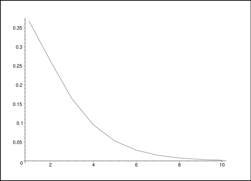
Figure 1: Probability $P(\infty,j)$, for $j=1$,…, $10$

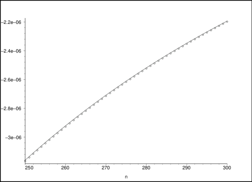
$\circ$  : $M(n)-M(\infty)-C_{1}/n$

— : $C_{2}/n^{2}$

Figure 2: Convergence of $M(n)$ to $M(\infty)$, for $n=250$,…, $300$

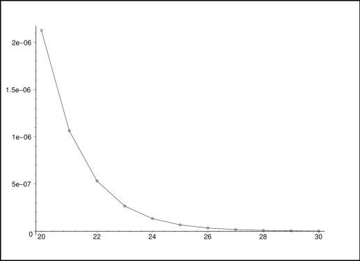
$\circ$  : Observed values of $P(\infty,j)$

— : Asymptotic approximation of $P(\infty,j)$ in (30)

Figure 3: $P(\infty,j)$ and its asymptotic approximation in (30) for large $j$ ($j=20$, …, $30$)

5 Is $1/n$ the optimal probability?

Let $t$ be a non negative real number. Following a question raised by J. Cardinal, let $t/n$ be the probability of choosing to participate in the election.

Is there one unique optimal real positive value $t^{*}$ in some real domain?

Taken in the initial context of the first leader election (“symmetry breaking”) protocol designed in [3, 4] (see Subsection 1.1), $t$ is introduced as a real non negative parameter which is assumed known to every processor on the ring.

Initially, all the processors are active. At the beginning of each current round of the election algorithm, every active processor knows $n$ (the counting process of $n$ is described in Subsection 1.1), and can decide with probability $t/n$ whether to become a candidate in the round. So, by definition, $t$ must a priori meet the condition $0\leq t/n\leq 1$.

The recurrence equation for the expectation $M(n,t)$ (with $0<t<2$) is similar to Eq. (1),

$$M(n,t) = 1\;+\;\left(1-\frac{t}{n}\right)^{n}M(n,t)$$ (31)

$$+ \sum_{k=2}^{n}{n\choose k}\left(\frac{t}{n}\right)^{k}\left(1-\frac{t}{n}\right)^{n-k}M(k,t)\ \quad\mbox{for}\ \;n\geq 2,$$ (33)

$$\mbox{and}\ \ M(1,t)=0\ \quad\mbox{(by definition)}.$$ (35)

Upon Differentiating Eq. (31) with respect to $t$, we obtain

$$M^{\prime}(n,t) = -\left(1-\frac{t}{n}\right)^{n-1}M(n,t)\;+\;\left(1-\frac{t}{n}\right)^{n}M^{\prime}(n,t)$$ (39)

$$+ \sum_{k=2}^{n}{n\choose k}\frac{k}{n}\,\left(\frac{t}{n}\right)^{k-1}\left(1-\frac{t}{n}\right)^{n-k}M(k,t)$$

$$- \sum_{k=2}^{n}{n\choose k}\left(\frac{t}{n}\right)^{k}\,\frac{n-k}{n}\,\left(1-\frac{t}{n}\right)^{n-k-1}M(k,t)$$

$$+ \sum_{k=2}^{n}{n\choose k}\left(\frac{t}{n}\right)^{k}\left(1-\frac{t}{n}\right)^{n-k}M^{\prime}(k,t)$$

Now, as in Eq. (12), an asymptotic approximation of $M(n,t)$ for large $n$ yields

$$M(\infty,t)\;=\;1\;+\;e^{-t}M(\infty,t)\;+\;\sum_{k\geq 2}e^{-t}\,\frac{t^{k}}{k!}\,M(k,t),$$ (40)

and, similarly, upon differentiating Eq. (40) with respect to $t$,

$$M^{\prime}(\infty,t) = -e^{-t}M(\infty,t)\;+\;e^{-t}M^{\prime}(\infty,t)\;+\;\sum_{k\geq 2}e^{-t}\,\frac{t^{k-1}}{(k-1)!}\,M(k,t)$$

$$+ \sum_{k\geq 2}e^{-t}\,\frac{t^{k}}{k!}\,M^{\prime}(k,t)\;-\;\sum_{k\geq 2}e^{-t}\,\frac{t^{k}}{k!}\,M(k,t)$$

or

$$M^{\prime}(\infty,t)\;=\;1\;-\;M(\infty,t)\;+\;e^{-t}M^{\prime}(\infty,t)\;+\;\sum_{k\geq 2}e^{-t}\,\frac{t^{k-1}}{(k-1)!}\,M(k,t)\;+\;\sum_{k\geq 2}e^{-t}\,\frac{t^{k}}{k!}\,M^{\prime}(k,t).$$ (41)

Note that the same expression of $M^{\prime}(\infty,t)$ can also be derived from the recurrence Eq. (39) by using asymptotic expansions similar to the ones given in Section 2.

5.1 Optimal probability on the domain $(0,2)$

A numerical study of the equation $M^{\prime}(\infty,t)=0$ on the open segment $U=\;(0,2)$ easily leads to the solution.

$$t^{*}=1.0654388051\ldots,\ \quad\mbox{with}\ \qquad M(\infty,t^{*})=2.4348109638268515517966\ldots$$

The relative gain on $M(\infty,1)$ is a bit larger than $.0028278945$ (hardly more than $.28$ %).

Since the (necessary) condition $M^{\prime}(\infty,t^{*})=0$ is not sufficient for $M(\infty,t)$ to have an extremum at $t^{*}$, there remains to prove

1. that $M(\infty,t)$ has a minimum at $t^{*}\in U$,

2. that this minimal solution $t^{*}$ is indeed unique on the segment $(0,2)$.

Both results derive from the following Subsection 5.1.1.

5.1.1 $M(\infty,t)$ is a strictly convex function on the segment $(0,2)$

All definitions regarding real and convex functions that are used in the following may be found in [8, Chap. 1 and 3].

Since a strictly convex function on some real segment admits at most one global minimum on that segment, both above results (1 and 2) are shown simultaneously by proving that $M(\infty,t)$ is indeed a strictly convex positive real function in $U=(0,2)$.

For the sake of simplicity (and in the line of notations in Subsection 1.1), we let $M(\infty,t)$ denote $\displaystyle\lim_{n\to\infty}M(n,t)$,

$$b(n,k;t):=\;{n\choose k}\left(\frac{t}{n}\right)^{k}\left(1-\frac{t}{n}\right)^{n-k},$$

and finally, we also use the notation

$$\lambda(n,t):=\frac{1}{1-(1-t/n)^{n}-(t/n)^{n}}\ \qquad\mbox{for}\ \;n\geq 2.$$

Besides, the following form of the basic recurrence Eq. (31) is considered:

$$M(n,t)\;=\;\lambda(n,t)\;+\;\lambda(n,t)\,\sum_{k=2}^{n-1}b(n,k;t)\,M(k,t)\ \quad\mbox{and}\ \;M(1,t)=0.$$ (42)

Starting from the above recurrence Eq. (42), we show below by induction on $n$, that at any point $t\in U$ and for any integer $n\geq 2$ all functions $M(n,t)$ are strictly convex positive real functions.

Therefore, as the pointwise limit of such a sequence $\Big{(}M(n,t)\Big{)}_{n\geq 2}$ in $U$, $\displaystyle M(\infty,t):=\lim_{n\to\infty}M(n,t)$ will be itself a strictly convex positive real function in $(0,2)$ (see [8, p. 73]).

Note also that, by induction on $n$, all functions $M(n,t)$ $(n\geq 2)$ are in $\mathcal{C}^{\infty}(U,\mathbb{R})$ (i.e., infinitely differentiable in $(0,2)$), and this is also true for the limit $M(\infty,t)$. In the same line of argument, $\displaystyle M(n,0^{+}):=\lim_{t\to 0^{+}}M(n,t)=M(n,2^{-}):=\lim_{t\to 2^{-}}M(n,t)=+\infty$ for any integer $n\geq 2$, which remains true in the limit $M(\infty,t)$.

$\bullet$ Basic step. Whenever $n=2$, and $n=3$, Eq. (31) yields

$$M(2,t)=\;\frac{2}{t(2-t)}\ \quad\mbox{and}\ \quad M(3,t)=\;\frac{18-3t-2t^{2}}{3t(2-t)(3-t)}\,.$$

So when $k=2$ and $k=3$, $M(k,t)$ are two positive functions in $\mathcal{C}^{\infty}(U,\mathbb{R})$ s.t. $M(k,0^{+})=M(k,2^{-})=+\infty$.

Moreover, since

$$M^{\prime\prime}(2,t) = 4\;\frac{3t^{2}-6t+4}{t^{3}(2-t)^{3}}\;\geq M^{\prime\prime}(2,1)=4\ \qquad\mbox{and}$$

$$M^{\prime\prime}(3,t) = -2\;\frac{2t^{6}+9t^{5}-189t^{4}+837t^{3}-1674t^{2}+1620t-648}{3t^{3}(2-t)^{3}(3-t)^{3}}\;>3,$$

$M(2,t)$ and $M(3,t)$ are two strictly convex functions in $U$.

$\bullet$ Induction Hypothesis. Assume now that for all $t\in U$, every function $M(k,t)$ is a strictly convex positive real function in $\mathcal{C}^{\infty}(U,\mathbb{R})$, s.t. $M(k,0^{+})=M(k,2^{-})=+\infty$ for any integer $2\leq k<n$.

At any point $t\in U$, $\lambda(n,t)\geq 1$ for any positive integer $n$ and $b(n,k;t)\geq 0$ for any pair $(k,n)$ of non negative integers.

In virtue of Eq. (42) and the induction hypothesis, $\displaystyle\lambda(n,t)\,\sum_{k=2}^{n-1}b(n,k;t)M(k,t)$ is a linear combination of strictly convex (positive real) functions with non negative coefficients, $\lambda(n,t)\times b(n,k;t)$, in $U$.

Furthermore, $\lambda(n,t)$ in infinitely differentiable in $U$, $\displaystyle\lim_{t\to 0^{+}}\lambda(n,t)=+\infty$ and $\lambda(n,2)$ is bounded (except for $n=2$, since $\lambda(2,2^{-})=+\infty$).

Next, there remains to prove that $\Big{(}\lambda(n,t)\Big{)}_{n\geq 2}$ is also a sequence of strictly convex positive real function in $U$.

For any given $0<t<2$ and for any $n\geq 2$, the value $\lambda(n,t)$ enjoys the two following inequalities, which derive from the tight inequalities shown in [9, p. 242]: for $0\leq t/n<1$,

$$\left(1\;-\;e^{-t}\left(1-\frac{t^{2}}{n}\right)\;-\;\frac{t^{2}}{n^{2}}\right)^{-1}\;\leq\;\lambda(n,t)\;\leq\;\left(1\;-\;e^{-t}\;-\;\frac{t^{n}}{2^{n}}\right)^{-1}.$$ (43)

It is easily seen that, for any fixed value of $t\in U$, $\lambda(n,t)$ $(n\geq 2)$ is a strictly increasing sequence, and $\displaystyle\lim_{n\to\infty}\lambda(n,t)=\frac{1}{1-e^{-t}}\,$.

On the other hand, $\lambda(n,t)$ is a strictly decreasing function of $t\in U$ for any fixed $n\geq 2$.

In short, since $\lambda^{\prime\prime}(2,t)\geq 4$ and $\lambda^{\prime\prime}(3,t)\geq 32/27$, $\lambda(2,t)$ and $\lambda(3,t)$ are two strictly convex positive real function in $\mathcal{C}^{\infty}(U,\mathbb{R})$.

Again, the proof is by induction on $n$. If we assume (Induction hypothesis) that, up to any integer $n\geq 2$, $\lambda(n,t)$ is a strictly convex function of $t$ in $U$, then $\lambda(n+1,t)$ is indeed a strictly convex function of $t$ on $U$. For example, assuming that $\lambda^{\prime\prime}(n,t)>0$ for any integer $n\geq 2$, it is shown after some algebra that $\lambda^{\prime\prime}(n+1,t)\geq\lambda^{\prime\prime}(n,t)>0$, by the above two inequalities in Eq. (43) and their resulting properties on $\lambda(n,t)$.

Thus, the positive sequence $\Big{(}\lambda(n,t)\Big{)}_{n\geq 2}$ is also composed of strictly convex real function in $U$

Finally, Eq. (42) and the above results show that, for all $t\in U$ and for any integer $n\geq 2$, $M(n,t)$ is a linear combination of strictly convex (positive real) functions with non negative coefficients: $\lambda(n,t)$ and $\lambda(n,t)\times b(n,k;t)$.

Hence, $\Big{(}M(n,t)\Big{)}_{n\geq 2}$ is a sequence of strictly convex positive real functions in $\mathcal{C}^{\infty}(U,\mathbb{R})$, s.t. $M(n,0^{+})=M(n,2^{-})=+\infty$.

In conclusion, $M(\infty,t)$ is the pointwise limit of the strictly increasing sequence $\Big{(}M(n,t)\Big{)}_{n\geq 2}$ of strictly convex positive real functions of $t\in U$ (see [8, p. 73]). Therefore, $M(\infty,t)$ is also strictly convex in $(0,2)$, and the value $M(\infty,t^{*})$ at $t^{*}=1.065439\ldots$, is the unique global minimum of $M(\infty,t)$ on this segment and we are done. A plot of $M(\infty,t)$ is given in Fig. 4.

In that sense, we answered the question set in Section 5: on the real domain $(0,2)$, $t^{*}\!/n$ is indeed the unique optimal probability for an active processor to choose and participate in the election.

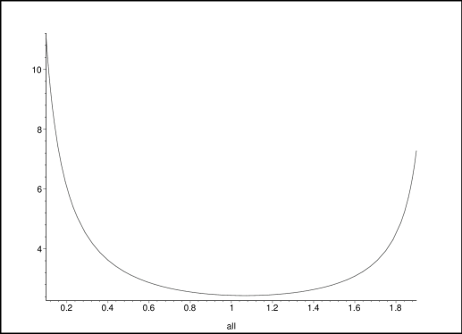
Figure 4: $M(\infty,t),\ t\in(0,2)$

Remark 5.1

For any integer $n\geq 2$, $M(n,t)$ is twice differentiable for all $t\in(0,2)$. Hence, if $M^{\prime\prime}(n,t)>0$ the functions $M(n,t)$ are all strictly convex; but the converse is not true.

The positive real function $M(\infty,t)$ is defined on the real segment $U=(0,2)$ as the pointwise limit of strictly convex positive real functions defined in $U$. Such is a sufficient condition for $M(\infty,t)$ to be also strictly convex in $U$. However the condition is not necessary.

Furthermore, $M(\infty,t)$ is the uniform limit of real functions on any compact subset of the segment $(0,2)$. This is another way of deriving that sequences of strictly convex functions do remain strictly convex in the limit on any compact subinterval of $(0,2)$.

6 What happens to $M(\infty,t)$ when $t\geq 2$?

There remains to investigate how $M(\infty,t)$ varies as a function of $t\geq 2$. In the first place, we just assume that the real parameter $t$ belongs to the domain $(2,3)$.

6.1 Variation of $M(\infty,t)$ in the domain $[2,3)$

Since $t\in(2,3)$ and $0\leq t/n\leq 1$ (by definition), the value of the function $M(n,t)$ must be handled separately in the case when $n=2$ (i.e. on a ring with two processors).

More precisely, two situations may then occur, in which the symmetry cannot be broken with the original algorithm (see [4, p. 1]:

• if $t=2$, $M(2,2)=b(2,2;2)=1$. Both active processors on the ring decide with probability $1$ to become candidates in each round, and the protocol either perfoms an election with two leaders, or enters an infinite computation;

• if $2<t<3$, we must also set $M(2,t)=1$ for the consistency of definitions (when $t\to 3^{-}$, $M(2,3^{-})=+\infty$, as is shown below). In such a case no termination of the protocol can be achieved.

Since $M(2,t)=1$ is set for all $t\in(2,3)$, the recurrence equation for the expectation $M(n,t)$ is expressed in a slightly different form from Eqs. (31) and (42) on the segment $[2,3)$.

$$M(n,t)\;=\;\lambda(n,t)\;+\;\lambda(n,t)\,b(n,2;t)\;+\;\lambda(n,t)\,\sum_{k=3}^{n-1}b(n,k;t)\,M(k,t)\ \quad\mbox{and}\ \;M(2,t)=1,$$ (44)

where, according to the notation in Subsection 5.1.1,

$$b(n,2;t):=\;{n\choose 2}\left(\frac{t}{n}\right)^{2}\left(1-\frac{t}{n}\right)^{n-2},\ \quad\mbox{and}\ \quad\lambda(n,t):=\;\frac{1}{1-(1-t/n)^{n}-(t/n)^{n}}\ \quad\mbox{for}\ \;n\geq 3.$$

There remains to prove that $M^{\prime}(\infty,t)>0$ on the segment $[2,3)$, with $M(\infty,3^{-})=+\infty$.

First, following Subsection 5.1.1 (i.e. again by induction on $n\geq 3$), $M(n,t)$ in Eq. (44) is easily shown to be an increasing sequence of $n\geq 3$ for fixed $t$ in $[2,3)$.

Thus, for all $n\geq 3$ and for any $t\in[2,3)$, $M(n,t)\leq M(n,t)\leq M(\infty,t)$.

Next, by (modified) Eq. (40) with $n\geq 3$ and $t\in[2,3)$, upper and lower bounds on $M(\infty,t)$ are derived.

More precisely, after few computations the following two inequalities hold for all $t\in[2,3)$,

$$M(\infty,t) \leq \frac{2e^{-t}}{t(t+2)}\;+\;\frac{t}{t+2}$$ (45)

$$M(\infty,t) \geq \frac{1}{1-e^{-t}}\left(1\;+\;\frac{1}{2}t^{2}e^{-t}\;+\;M(3,t)\,e^{-t}(e^{t}-t^{2}/2-t-1)\right),$$ (46)

where $\displaystyle M(3,t)=\frac{9-3t^{2}-t^{3}}{3t(3-t)}\,$.

(Note that since $2.2797\ldots\leq M(\infty,2)\leq 2.34726\ldots$, both inequalities (45) and (46) make sense.)

Finally, Eqs. (45) and (46) are used to bound $M^{\prime}(\infty,t)$ from below, and derive that $M^{\prime}(\infty,t)>0$ on the segment $[2,3)$.

Indeed, by (modified) Eq. (41) with $t\in[2,3)$, a few calculations yield a lower bound on $M^{\prime}(\infty,t)$ for any $t\in[2,3)$.

$$M^{\prime}(\infty,t)\geq\;\frac{2e^{t}}{t(t+2)}\;-\;\frac{2e^{t}(2e^{t}+t^{2})}{t^{2}(t+2)^{2}}\;+\;\frac{2(e^{t}-t-1)(9-3t^{2}-t^{3})}{3t(t+2)(3-t)}\,.$$ (47)

And, since $M^{\prime}(\infty,t)>2.26605840\ldots$ for all $t\in[2,3)$, $M^{\prime}(\infty,t)>0$ on that segment. Furthermore, since all functions $M(n,t)$ $(n\geq 3)$ are in $\mathcal{C}^{\infty}([2,3),\mathbb{R})$ (see Subsection 5.1.1), $M(\infty,3^{-})=+\infty$ holds for all $t\in[2,3)$.

Hence, $M(\infty,t)$ is strictly increasing on the segment $(2,3)$ and $M(\infty,3^{-})=+\infty$.

The curve $M(\infty,t)$ is represented in Fig. 5 on the segment $[2,3)$.

Figure 5: $M(\infty,t),\ t\in[2,3)$

6.2 Variation of $M(\infty,t)$ in the domains $(\xi,\xi+1)$, with $\xi\geq 3$

Investigating the variation of the functions $M(\infty,t)$ when $t\geq 3$ can be carried out along the same lines as in the previous Subsection 6.1.

As can be noticed (e.g. in Subsection 5.1.1), the only poles of the functions $M(n,t)$ are all the non negative integers 0, 2, 3,… (1 excepted) on the real line. Thus, the variation of $M(\infty,t)$ when $t\geq 3$ must be considered on all such consecutive real segments $(\xi,\xi+1)$, where the $\xi$’s are all integers $\geq 3$.

Since $t\in(\xi,\xi+1)$ still meets the condition $0\leq t/n\leq 1$ (by definition), each value $M(\xi,t)$ must again be handled separately on each open segment $I=(\xi,\xi+1)$.

More precisely, whenever $n=\xi$ there are $\xi$ processors on the ring, and the condition $0\leq t/\xi\leq 1$ must still hold. The situation is similar to the one in Subsection 6.1: the original algorithm cannot break the symmetry, neither if $t=\xi$, nor if $\xi<t<\xi+1$ (see [4, p. 1]).

To overcome the difficulty, and for the sake of the consistency of the definitions, we set $M(\xi,t):=\lceil\lg(\xi)\rceil$ for all $t\in I$, with $\xi\geq 3$. For example, $M(3,t):=2$ (by definition) on the open segment $(3,4)$, and the recurrence for the expectation $M(n,t)$ is slightly different from Eq. (44) if $t\in(3,4)$.

Similarly, each basic recurrence equation for $M(n,t)$ (Eq. (44)), $M^{\prime}(n,t)$ (Eq. (39)), $M(\infty,t)$ (Eq. (40)) and $M^{\prime}(\infty,t)$ (Eq. (41)) must be adapted to the conditions on each segment $I$ considered.

On each open segment $I=(\xi,\xi+1)$ ($\xi\geq 3$), the variation of the real function $M(\infty,t)$ is roughly the same. In particular, $M(\infty,t)$ is monotone increasing in $I$, and it admits no minimum on each such segments.

7 Conclusions

As pointed out in the Introduction, performing the asymptotic analyses of various recurrence relations brings into play some basic, though powerful, analytic techniques. This is the reason why such methods make it possible to find easily all moments of the algorithm asymptotic “cost” (the numbers of rounds required), especially $M(\infty)$ and $M^{(2)}(\infty)$ (when $n$ gets sufficiently large), as well as an asymptotic approximation of $P(\infty,j)$ (when $j\to\infty$). The latter is derived by computing singular expansions of generating functions around their smallest singularity. Asymptotic expansions of all moments can also be mechanically derived. All the numerical results performed (with Maple) by both techniques are quite accurate and fit in perfectly.

Generalizing to a probability $t/n$, where $t$ is a positive real number, shows that there exists one unique minimum of the function $M(\infty,t)$ on the real segment $(0,2)$ : $M(\infty,t^{*})=2.434810964\ldots$ at the point $t^{*}=1.065439\ldots$ Besides, the variation of $M(\infty,t)$ whenever $t\geq 2$ shows quite the same behaviour on each real open interval $(\xi,\xi+1)$, where the $\xi$’s are all the integers $\geq 2$.

In the asymptotic analysis, the major difficulty arises from the proof of interchanging the limits and the summations in the recurrences. Two different methods are given that may be used in many other similar situations: the Laplace method for sums, which requires the use of asymptotics via the Saddle point technique, and the Lebesgue’s dominated convergence property.

In conclusion, such analytic techniques may serve as basic bricks for finding the asymptotic complexity measures of quite a lot of other algorithms, in distributed or sequential settings.

References

- [1] C.M. Bender, S.A. Orzag, Advanced Mathematical Methods for Scientists and Engineers, McGraw-Hill, 1978.
- [2] J.A. Fill, H. Mahmoud, W. Szpankowski, On the Distribution for the Duration of a Randomized Leader Election Algorithm, Annals of Applied Probability, 1, 1260-1283, 1996.
- [3] A. Itai, M. Rodeh, Symmetry Breaking in Distributed Networks, Proc. of the 2nd IEEE Symp. on Found. of Comp. Science, (FOCS), 150-158, 1981.
- [4] A. Itai, M. Rodeh, Symmetry Breaking in Distributed Networks, Information and Computation, 88(1), 60-87, 1990.
- [5] D.E. Knuth, The Art of Computer Programming - Sorting and Searching, vol. 3, Addison-Wesley, 1973.
- [6] G. Louchard, H. Prodinger, The Moments Problem of Extreme-Value Related Distribution Function, , available at: http://www.ulb.ac.be/di/mcs/louchard/mom7.ps.
- [7] H. Prodinger, How to Select a Loser?, Discrete Math., 120, 149-159, 1993.
- [8] W. Rudin, Real and Complex Analysis, 2nd Edition, McGraw-Hill, 1974.
- [9] E.T. Whittaker and G.N. Watson, A Course in Modern Analysis, Cambridge University Press, 1965.