Slepian-Wolf Code Design via Source-Channel Correspondence

Abstract

We consider Slepian-Wolf code design based on LDPC (low-density parity-check) coset codes for memoryless source-side information pairs. A density evolution formula, equipped with a concentration theorem, is derived for Slepian-Wolf coding based on LDPC coset codes. As a consequence, an intimate connection between Slepian-Wolf coding and channel coding is established. Specifically we show that, under density evolution, design of binary LDPC coset codes for Slepian-Wolf coding of an arbitrary memoryless source-side information pair reduces to design of binary LDPC codes for binary-input output-symmetric channels without loss of optimality. With this connection, many classic results in channel coding can be easily translated into the Slepian-Wolf setting.

I Introduction

Consider the problem of encoding $X$ with side information $Y$ at the decoder. Here $(X,Y)$ are two memoryless sources with joint probability distribution $P(x,y)$ on $\mathcal{X}\times\mathcal{Y}$. This is a special case of Slepian-Wolf coding. General cases can be reduced to this special case via either time-sharing or source splitting. For this special case, the Slepian-Wolf theorem states that the minimum rate for reconstructing $X$ is $H(X|Y)$. For simplicity, we assume $\mathcal{X}=\{0,1\}$ and $|\mathcal{Y}|<\infty$ throughout this paper. The general finite-alphabet case can be reduced to this special case via multilevel coding. In the literature many low-complexity Slepian-Wolf coding schemes have been proposed [2, 3, 4, 5], almost all of which are based on ideas from channel coding, and simply use some binary linear channel codes as Slepian-Wolf codes. In this approach it is implicitly assumed that a good channel code for a channel is also a good Slepian-Wolf code for the same channel linking the source and the side information; yet few justifications have been presented except for [6]. Motivated by these observations, in this paper we consider Slepian-Wolf code design based on binary LDPC coset codes (see Section II for details). To this end we derive the density evolution formula for Slepian-Wolf coding, equipped with a concentration theorem. An intimate connection between Slepian-Wolf coding and channel coding is then established. Specifically we show that, under density evolution, any Slepian-Wolf source coding problem, where the joint distribution $P(x,y)$ can be arbitrary, is equivalent to a channel coding problem for a binary-input output-symmetric channel. Note that this channel is often different from the channel between the source and the side information in the original Slepian-Wolf coding problem. This is in sharp contrast to the practice in the works reviewed above where the two channels are assumed the same.

The rest of this paper is organized as follows. In Section II, we review some basic results in the channel coding theory. The emphasis will be on binary linear codes with the practical belief-propagation decoding algorithm. In Section III, we develop the belief-propagation algorithm for Slepian-Wolf coding. The associated density evolution formula and concentration theorem are also provided. An intimate connection between Slepian-Wolf coding and channel coding under density evolution is established in Section IV. We conclude the paper in Section V.

II Review of Channel Coding Theory

Any binary linear code $\mathcal{C}=\{\mathbf{c}\}$ can be expressed as the set of solutions $\mathbf{c}$ to a parity check equation $H\mathbf{c}=\mathbf{0}$, where $H$ is called the parity check matrix of $\mathcal{C}$, and here multiplication and addition are modulo 2. Given some general syndrome $\mathbf{s}\in\{0,1\}^{n-k}$, the set of all $n$-length vectors $\mathbf{x}$ satisfying $H\mathbf{x}=\mathbf{s}$ is called a coset $\mathcal{C}_{\mathbf{s}}$. A $(d_{v},d_{c})$-regular low-density-parity-check (LDPC) code is a binary linear code determined by the condition that every codeword bit participates in exactly $d_{v}$ parity-check equations and that every such check equation involves exactly $d_{c}$ codeword bits. Given the parity check matrix $H$, we can construct a bipartite graph with $n$ variable nodes and $m=n-k$ check nodes. Each variable node corresponds to one bit of the codeword, and each check node corresponds to one parity-check equation. Edges in the graph connect variable nodes to check nodes and are in one-to-one correspondence with the nonzero entries of $H$. The ensemble $\mathcal{C}^{n}(d_{v},d_{c})$ of $(d_{v},d_{c})$-regular LDPC codes of length $n$ is defined in [7]. We can also define the irregular code ensemble $\mathcal{C}^{n}(\lambda,\rho)$, where $(\lambda,\rho)$ denotes a degree distribution pair [7].

The belief-propagation algorithm is an iterative message-passing algorithm. Let $m^{(l)}_{vc}$ denote the message sent from variable node $v$ to its incident check node $c$ in the $l$th iteration. Similarly, let $m^{(l)}_{cv}$ denote the message sent from check node $c$ to its incident variable node $v$ in the $l$th iteration. The update equations for the messages under belief propagation are described below:

$$m^{(l)}_{vc}=\left\{\begin{array}[]{ll}m_{0},&\mbox{if }l=0\\ m_{0}+\sum\limits_{c^{\prime}\in C_{v}\setminus\{c\}}m^{(l)}_{c^{\prime}v},&\mbox{if }l\geq 1\\ \end{array}\right.$$

$$m^{(l)}_{cv}=\gamma^{-1}\left(\sum\limits_{v^{\prime}\in V_{c}\setminus\{v\}}\gamma\left(m^{(l-1)}_{v^{\prime}c}\right)\right).$$

where $C_{v}$ is the set of check nodes incident to variable node $v$, $V_{c}$ is the set of variable nodes incident to check node $c$, $m_{0}\triangleq\ln\frac{P(y_{i}|x_{i}=0)}{P(y_{i}|x_{i}=1)}$ is the initial message associated with the variable node $v$, and $\gamma(x)=\left(\textrm{sgn}(x),-\ln\tanh\left|\frac{x}{2}\right|\right)$.

The performance of LDPC codes under the belief-propagation algorithm is relatively well-understood for binary-input output-symmetric (BIOS) channels.

Definition 1

A binary input channel with transition probability function $p(\cdot|\cdot):{\cal X}\times{\cal Y}\to[0,1]$ from ${\cal X}$ to ${\cal Y}$ is output-symmetric if there exists an injective map $\varphi:\mathcal{Y}\rightarrow\mathbb{R}$ such that

$$p(\varphi(y_{t})=\varphi(y)|x_{t}=0)=p(\varphi(y_{t})=-\varphi(y)|x_{t}=1),\forall y\in\mathcal{Y},$$

where $y_{t}$ is the channel output in response to channel input $x_{t}$.

An important property of the BIOS channel is that under the belief-propagation algorithm, the decoding error probability is independent of the transmitted codeword. So without loss of generality, we can assume the all-zero codeword is transmitted.

In order to analyze the asymptotic (in codeword length) performance of the LDPC code ensemble $\mathcal{C}^{n}(\lambda,\rho)$, a powerful technique called density evolution is developed in [8, 9]. The iterative density evolution formula for BIOS channels is given in the following theorem.

Theorem 1 ([9], Theorem 2)

For a given BIOS memoryless channel let $P^{(0)}$ denote the initial message density of log-likelihood ratios, assuming that the all-zero codeword was transmitted. If, for a fixed degree distribution pair $(\lambda,\rho)$, $P^{(l)}$ denotes the density of the messages passed from the variable nodes to the check nodes at the $l$th iteration of belief propagation then, under the independence assumption

$$P^{(l)}=P^{(0)}\otimes\lambda(\Gamma^{-1}(\rho(\Gamma(P^{(l-1)}))))$$ (2)

where $\Gamma$ is the density transformation operator induced by $\gamma$.

The theorem below provides a theoretical foundation of density evolution.

Theorem 2 ([8], Theorem 2)

Over the probability space of all graphs $\mathcal{C}^{n}(d_{v},d_{c})$ and channel realizations let $Z$ be the number of incorrect messages among all $nd_{v}$ variable-to-check node messages passed at iteration $l$. Let $p^{(l)}_{e}$ be the expected number of incorrect messages passed along an edge with a tree-like directed neighborhood of depth at least $2l$ at the $l$th iteration, i.e.,

$$p^{(l)}_{e}=\int_{-\infty}^{0^{-}}P^{(l)}(dm)+\frac{1}{2}\int_{0^{-}}^{0^{+}}P^{(l)}(dm).$$

Then, there exist positive constants $\beta=\beta(d_{v},d_{c},l)$ and $\gamma=\gamma(d_{v},d_{c},l)$ such that for any $\epsilon>0$ and $n>\frac{2\gamma}{\epsilon}$ we have

$$\mbox{Pr}\{|Z-nd_{v}p^{(l)}_{e}|>nd_{v}\epsilon\}\leq 2e^{-\beta\epsilon^{2}n}.$$

The main contribution of this paper is that we prove a similar density evolution formula with an associated concentration theorem for Slepian-Wolf coding, and establish an intimate connection between Slepian-Wolf coding and channel coding under density evolution.

For a given joint distribution $P(x,y)$ on $\mathcal{X}\times\mathcal{Y}$, we can define two channels: one from $X$ to $Y$ with transition probability $P(y|x)$, the other from $Y$ to $X$ with transition probability $P(x|y)$. Both channels are somehow related to Slepian-Wolf coding as we shall discuss in the following two examples:

Example 1 (Channel from $Y$ to $X$)

Suppose $X=Y\oplus Z$, where $X,Y$ and $Z$ all assume values in $\{0,1\}$, $\oplus$ is the modulo-2 addition, and $Z\sim\mbox{Ber}(q)$ (with $0\leq q\leq\frac{1}{2}$) is independent of $Y$. Let $H$ be an $(n,k)$ binary parity-check matrix. Let $\mathcal{C}$ (i.e., $\mathcal{C}_{0}$) be the linear code with the parity check matrix $H$. Assuming that all rows of $H$ are linearly independent, there are $2^{k}$ codewords in $\mathcal{C}$, so the code rate is $(\log|\mathcal{C}|)/n=k/n$.

The following scheme was suggested by Wyner [6]. Given $\mathbf{x}$, the encoder sends the syndrome $\mathbf{s}=H\mathbf{x}$ to the decoder. With the side information $\mathbf{y}$, the decoder can compute $H\mathbf{z}=H\mathbf{x}\oplus H\mathbf{y}=\mathbf{s}\oplus H\mathbf{y}$. Syndrome decoding can be implemented to find the minimum weight $\hat{\mathbf{z}}$ such that $H\hat{\mathbf{z}}=H\mathbf{z}$. The decoder then claims that $\hat{\mathbf{x}}=\mathbf{y}+\hat{\mathbf{z}}$ is the target sequence $\mathbf{x}$. It can be shown that if the error probability of $\mathcal{C}$ when used over the channel from $Y$ to $X$ (i.e., a binary symmetric channel with crossover probability $q$) under syndrome decoding is $\epsilon$, then the above Slepian-Wolf coding scheme is also of error probability $\epsilon$. Furthermore, if $\mathcal{C}$ is capacity-achieving for the channel from $Y$ to $X$, i.e, the rate of $\mathcal{C}$ is $1-H(q)$, then the rate of this Slepian-Wolf coding scheme is $H(q)$, which is exactly the Slepian-Wolf limit.

Example 2 (Channel from $X$ to $Y$)

Suppose $X$ is uniformly distributed over $\{0,1\}$ and $P(y|x)$ is a BIOS channel.

The encoding procedure is the same as that in Example 1. Given $\mathbf{x}$, the encoder finds the coset $C_{\mathbf{s}}$ that contains $\mathbf{x}$ and send the syndrome $\mathbf{s}$ to the decoder. So the encoder rate is $(n-k)/n$. Given the side information $\mathbf{y}$, the decoder tries to recover $\mathbf{x}$ using the belief propagation decoding algorithm for $C_{\mathbf{s}}$. For a BIOS channel, the decoding error probability is the same for all coset codes $\mathcal{C}_{\mathbf{s}}$ under the belief-propagation algorithm. So if $\mathcal{C}_{\mathbf{0}}$ is a linear code for channel $P(y|x)$ with error probability $\epsilon$ under belief-propagation decoding, then the error probability of the above Slepian-Wolf coset coding scheme is also $\epsilon$. Furthermore, assuming $\mathcal{C}_{\mathbf{0}}$ is a capacity achieving linear code for channel $P(y|x)$, the above coding scheme is then of rate $1-C=H(X|Y)$, which is exactly the Slepian-Wolf limit. Here $C$ is the capacity of channel $P(y|x)$.

When $X$ is nonuniform, we can still use the above coset coding scheme as long as $\mathcal{C}_{\mathbf{0}}$ is a good channel code for channel $P(y|x)$ under the belief-propagation decoding algorithm. The reason is that for a BIOS channel, the error probability resulting from the belief propagation decoding algorithm is the same for every codeword in every coset. Nonetheless, since $1-C>H(X|Y)$ when $X$ is nonuniform, we see that the above coset coding scheme fails to achieve the Slepian-Wolf limit even when $\mathcal{C}_{\mathbf{0}}$ is an optimal channel code for channel $P(x|y)$. This phenomenon has been observed in [10].

When $P(y|x)$ is not output-symmetric, the decoding error probability, under the belief-propagation algorithm, is in general different for different codewords in each coset, and also different for different cosets. In this case, the connection between channel coding for channel $P(y|x)$ and Slepian-Wolf coding is not clear.

We have seen that although the above two examples exhibit some interesting connections between channel coding (either for the channel from $X$ to $Y$ or the channel from $Y$ to $X$) and Slepian-Wolf coding, both of them have severe limitations. In this paper we shall provide a general framework, which includes these two examples as special cases, and within the framework establish the connection between channel coding and Slepian-Wolf coding. It should be emphasized that in our framework, $P(x)$ does not need to be uniform, and $P(y|x)$ does not need to be output-symmetric.

III Belief-Propagation Algorithm, Density Evolution and Concentration Theorem

We use the same encoding method as that in Example 1 and Example 2. We first fix a parity check matrix $H$. Given $\mathbf{x}$, the encoder sends the syndrome $\mathbf{s}=H\mathbf{x}$ to the decoder. But we do not use the channel decoding method in Example 2. The reason is that in channel coding, codewords are assumed to be equally probable, but in Slepian-Wolf coding, codewords are generated by $P(x)$, and are in general not equally probable if $X$ is not uniform over $\{0,1\}$. It turns out that it is easy to incorporate the prior distribution $P(x)$ into the belief-propagation. The update equations for the messages in this Slepian-Wolf decoding are described below:

$$m^{(l)}_{vc}=\left\{\begin{array}[]{ll}m_{0},&\mbox{if }l=0\\ m_{0}+\sum\limits_{c^{\prime}\in C_{v}\setminus\{c\}}m^{(l)}_{c^{\prime}v},&\mbox{if }l\geq 1\\ \end{array}\right.$$

$$m^{(l)}_{cv}=(-1)^{s}\gamma^{-1}\left(\sum\limits_{v^{\prime}\in V_{c}\setminus\{v\}}\gamma\left(m^{(l-1)}_{v^{\prime}c}\right)\right).$$ (4)

where $m_{0}\triangleq\ln\frac{P(x_{i}=0|y_{i})}{P(x_{i}=1|y_{i})}=\ln\frac{P(x_{i}=0,y_{i})}{P(x_{i}=1,y_{i})}$, and $s$ is the syndrome value associated with check node $c$. It can be verified that this algorithm produces the exact symbol-by-symbol a posteriori estimation of $\mathbf{x}$ given $\mathbf{y}$ when the underlying bipartite graph is a tree. We can see that the only difference from the channel decoding case is the definition of initial message $m_{0}$. This decoding scheme can be viewed as a MAP-version of the belief propagation algorithm, while the channel decoding scheme can be viewed as a ML-version of the belief propagation algorithm.

Now we proceed to develop the density evolution formula for this belief-propagation algorithm. We use the standard tree assumption. Let $P^{(l)}(x)$ $(x=0,1)$ be the message distribution from a variable node to a check node at the $l$th iteration conditioned on the event that the variable value is $x$. Similarly, let $Q^{(l)}(x)$ $(x=0,1)$ be the message distribution from a check node to a variable node at the $l$th iteration conditioned on the event that the target variable value is $x$. Assume $P(X=0)=p$. Let $\langle P^{(l)}\rangle=pP^{(l)}(0)+(1-p)P^{(l)}(1)\circ I^{-1}$, where $I(m)\triangleq-m$ is a parity reversing function. We have

$$p^{(l)}_{e}=\int_{-\infty}^{0^{-}}\langle P^{(l)}\rangle(dm)+\frac{1}{2}\int_{0^{-}}^{0^{+}}\langle P^{(l)}\rangle(dm),$$ (5)

where $p^{(l)}_{e}$ is the expected number of incorrect messages sent from a variable node at the $l$th iteration.

The following theorem provides a density-evolution formula for $\langle P^{(l)}\rangle$.

Theorem 3

Under the tree assumption,

$$\langle P^{(l)}\rangle=\langle P^{(0)}\rangle\otimes\lambda(\Gamma^{-1}(\rho(\Gamma(\langle P^{(l-1)}\rangle)))).$$ (6)

Remark: Theorem 3 does not directly follow from the approach in [9] since the all-zero codeword assumption is not valid in our setting.

Theorem 4 (Concentration Theorem)

Over the probability space of all graphs $\mathcal{C}^{n}(d_{v},d_{c})$ and source realizations let $Z$ be the number of incorrect messages among all $nd_{v}$ variable-to-check node messages passed at iteration $l$. Then, there exist positive constants $\beta=\beta(d_{v},d_{c},l)$ and $\gamma=\gamma(d_{v},d_{c},l)$ such that for any $\epsilon>0$ and $n>\frac{2\gamma}{\epsilon}$ we have

$$\mbox{Pr}\{|Z-nd_{v}p^{(l)}_{e}|>nd_{v}\epsilon\}\leq 2e^{-\beta\epsilon^{2}n}.$$

It can be verified that the density evolution formula (6) and concentration theorem (Theorem 4) do not depend on the definition of the initial message, i.e., they still hold if we replace $\langle P^{(0)}\rangle$ by an arbitrary probability distribution. This provides us a useful tool to study the problem of distribution mismatch. In many applications, the true source distribution cannot be estimated perfectly. For example, suppose $P(x,y)$ is the true source distribution and $P_{es}(x,y)$ is the estimated source distribution. The initial message is then given by $m_{0}=\log\frac{P_{es}(x=0|y)}{P_{es}(x=1|y)}$.

Let $P^{(l)}_{es}(x)$ $(x=0,1)$ be the density of the message from a variable node to a check node at the $l$th iteration conditioned on the event that the variable value is $x$. Let $\langle P^{(l)}_{es}\rangle=P(x=0)P^{(l)}_{es}(0)+P(x=1)P^{(l)}_{es}(1)\circ I^{-1}$. The density evolution formula of this mismatch problem is

$$\langle P^{(l)}_{es}\rangle=\langle P^{(0)}_{es}\rangle\otimes\lambda(\Gamma^{-1}(\rho(\Gamma(\langle P^{(l-1)}_{es}\rangle)))).$$ (7)

We can use the density evolution formula (7) to check whether the error probability goes to zero when the distribution mismatch occurs.

We have seen from Example 2 in Section II that under the ML-version of the belief-propagation decoding algorithm, the Slepian-Wolf coset coding scheme still works even if $X$ is nonuniform, as long as $\mathcal{C}_{\mathbf{0}}$ is a good channel code for channel $P(y|x)$ under the belief-propagation decoding algorithm. Actually, using the ML-version of the belief-propagation algorithm for decoding nonuniform $X$ can be viewed as a special case of distribution mismatch, where

$$\log\frac{P_{es}(x=0|y)}{P_{es}(x=1|y)}=\log\frac{P(y|x=0)}{P(y|x=1)},\quad\forall y\in\mathcal{Y}.$$

Thus in this example distribution mismatch does not imply decoding failure, but it may cause rate loss.

IV Source-Channel Correspondence

In the density evolution formula (2) in channel coding and density evolution formula (6) in Slepian-Wolf coding, the channel and source statistics come in only through the initial message distribution; all the remaining operations depend only on the degree distribution. So for a fixed degree distribution pair $(\lambda,\rho)$, if $P^{(0)}=\langle P^{(0)}\rangle$, then the two density evolutions are completely identical, i.e., we have $P^{(l)}=\langle P^{(l)}\rangle$ for all $l$. So a natural question is: For a given Slepian-Wolf initial message distribution $\langle P^{(0)}\rangle$, does there exist a BIOS channel whose initial message distribution $P^{(0)}$ is the same as $\langle P^{(0)}\rangle$? We now proceed to answer this question.

Definition 2 ([9], Definition 1)

We call a distribution $Q$ symmetric if $\int h(m)Q(dm)=\int e^{-m}h(-m)Q(dm)$ for any function $h$ for which the integral exists.

Lemma 1

$\langle P^{(l)}\rangle$ is symmetric.

Remark: The reason why $\langle P^{(l)}\rangle$ is symmetric even when there is no symmetry in the source distribution $P(x,y)$ is that the coset coding scheme is used, and the prior distribution $P(x)$ is incorporated in the decoding.

The following theorem is the main result of this section, which essentially says that under belief propagation decoding, for all $(X,Y)$ pairs, Slepian-Wolf code design with linear codes reduces to design of codes for certain symmetric channels.

Theorem 5

For any source distribution $P(x,y)$ on $\mathcal{X}\times\mathcal{Y}$ ($\mathcal{X}=\{0,1\},|\mathcal{Y}|<\infty$) with conditional entropy $H(X|Y)$, there exists a unique BIOS channel $P^{\prime}(y^{\prime}|x^{\prime})$ with capacity $C$ such that its initial message distribution $P^{(0)}$ is the same as the initial message distribution $\langle P^{(0)}\rangle$ induced by $P(x,y)$. Furthermore, we have $H(X|Y)+C=1$. The conversion from $P(x,y)$ to $P^{\prime}(y^{\prime}|x^{\prime})$ is given in Fig. 1.

Remark: It can be seen from Fig. 1 that $P^{\prime}(y^{\prime}|x^{\prime})$ is in general different from $P(y|x)$, and $P^{\prime}(y^{\prime}|x^{\prime})$ is symmetric even when $P(y|x)$ is not. Furthermore, if $P(x)$ is nonuniform, then $P^{\prime}(y^{\prime}|x^{\prime})$ is different from $P(y|x)$ even when $P(y|x)$ is symmetric.

\psfrag{p0}[r]{$p_{0}$}\psfrag{p1}[r]{$p_{1}$}\psfrag{q00}[c]{$q_{0,0}$}\psfrag{q10}[c]{$q_{1,0}$}\psfrag{q01}[c]{$q_{0,1}$}\psfrag{q11}[c]{$q_{1,1}$}\psfrag{q0n-2}[c]{$q_{0,n-2}$}\psfrag{q1n-2}[c]{$q_{1,n-2}$}\psfrag{q0n-1}[c]{$q_{0,n-1}$}\psfrag{q1n-1}[c]{$q_{1,n-1}$}\psfrag{p0q00}[c]{$p_{0}q_{0,0}$}\psfrag{p1q10}[c]{$p_{1}q_{1,0}$}\psfrag{p0q01}[c]{$p_{0}q_{0,1}$}\psfrag{p1q11}[c]{$p_{1}q_{1,1}$}\psfrag{p0q0n-1}[c]{$p_{0}q_{0,n-1}$}\psfrag{p1q1n-1}[c]{$p_{1}q_{1,n-1}$}\psfrag{dots}[c]{\Large$\cdots$}\psfrag{vdots}[c]{\Large$\vdots$}\includegraphics[scale={0.5}]{sccorrespondence}

Figure 1: Source-to-channel conversion

Let $\mbox{Ch}(\cdot)$ be the function that maps $P(x,y)$ to $P^{\prime}(y^{\prime}|x^{\prime})$. It turns out this function is not invertible.

Definition 3 (Equivalence)

Two sources distributions, $P(x,y)$ and $P^{\prime}(x^{\prime},y^{\prime})$, are equivalent if they induce the same initial message distribution $\langle P^{(0)}\rangle$ (or if $\mbox{Ch}(P(x,y))=\mbox{Ch}(P^{\prime}(x^{\prime},y^{\prime}))$).

For a symmetric distribution $Q$ given by $Q\left(\ln\frac{a_{i}}{a_{n-1-i}}\right)=a_{i}$, $i=0,1,\cdots,n-1$, where $a_{i}\in(0,1]$ and $\sum_{i=0}^{n-1}a_{i}=1$, we can compute all source distributions for which the induced initial message distribution $\langle P^{(0)}\rangle$ is equal to $Q$. These can be written (possibly after relabelling) in the following parametric form:

$$P(y=i) = \alpha_{i}(a_{i}+a_{n-1-i}),$$ (8)

$$P(x=0|y=i) = \frac{a_{i}}{a_{i}+a_{n-1-i}},$$ (9)

$$P(x=1|y=i) = \frac{a_{n-1-i}}{a_{i}+a_{n-1-i}},i=0,\cdots,n-1.$$ (10)

where $\alpha_{i}\in[0,1]$, $1-\alpha_{i}=\alpha_{n-1-i}$, $i=0,1,\cdots,n-1$. So for a fixed initial message distribution with $n$ probability mass points, the set of equivalent source distributions has totally $\lfloor\frac{n}{2}\rfloor$ degrees of freedom. This should be contrasted with the $2n-2$ degrees of freedom for source distributions (over $\mathcal{X}\times\mathcal{Y}$ with $|\mathcal{X}|=2$ and $|\mathcal{Y}|=n$) under the conditional entropy constraint. We can also see that the equivalent source distributions must have the same reverse channel $P(x|y)$; the freedom comes only from $P(y)$.

Example 3

Consider the following class of source distributions $P(y=e)=\epsilon$, $P(y\in\{0,1\})=1-\epsilon$, $P(x=i|y=i)=1$, $i=0,1$, $P(x=0|y=e)=P(x=1|y=e)=\frac{1}{2}$. It is easy to verify that this class of source distributions is an equivalence class. In fact, for any distribution $P(x,y)$ in this class, $\mbox{Ch}(P(x,y))$ is the binary erasure channel with erasure probability $\epsilon$. Since the capacity of the binary erasure channel can be achieved with LDPC codes under the belief-propagation decoding algorithm, it follows that for distributions in this class, the Slepian-Wolf limit is achievable with the LDPC coset coding scheme under belief-propagation decoding.

Example 4

It can be verified that for fixed $q$, the source distributions in Example 1 are all equivalent.

Given two channels, $P(y|x)$ and $P^{\prime}(y^{\prime}|x^{\prime})$, we say $P^{\prime}(y^{\prime}|x^{\prime})\preceq P(y|x)$ if $P^{\prime}(y^{\prime}|x^{\prime})$ is physically degraded with respect to $P(y|x)$. We now generalize this concept to source distributions.

Definition 4 (Monotonicity)

Given two source distributions, $P(x,y)$ and $P^{\prime}(x^{\prime},y^{\prime})$, we say $P^{\prime}(x^{\prime},y^{\prime})\preceq P(x,y)$ if $\mbox{Ch}(P^{\prime}(x^{\prime},y^{\prime}))\preceq\mbox{Ch}(P(x,y))$.

Remark: One may tend to define “monotonicity” in the following way: $P^{\prime}(x^{\prime},y^{\prime})\preceq P(x,y)$ if (possibly after relabelling) $P^{\prime}(x)=P(x)$ for all $x\in\mathcal{X}$ and $P^{\prime}(y^{\prime}|x^{\prime})$ is physically degraded with respect to $P(y|x)$. It turns out the “monotonicity” in this sense also satisfies the condition $\mbox{Ch}(P^{\prime}(x^{\prime},y^{\prime}))\preceq\mbox{Ch}(P(x,y))$, as illustrated in Fig. 2.

\psfrag{p0}[r]{$p_{0}$}\psfrag{p1}[r]{$p_{1}$}\psfrag{q00}[c]{$q_{0,0}$}\psfrag{q10}[c]{$q_{1,0}$}\psfrag{q01}[c]{$q_{0,1}$}\psfrag{q11}[c]{$q_{1,1}$}\psfrag{q0n-2}[c]{$q_{0,n-2}$}\psfrag{q1n-2}[c]{$q_{1,n-2}$}\psfrag{q0n-1}[c]{$q_{0,n-1}$}\psfrag{q1n-1}[c]{$q_{1,n-1}$}\psfrag{p0q00}[c]{$p_{0}q_{0,0}$}\psfrag{p1q10}[c]{$p_{1}q_{1,0}$}\psfrag{p0q01}[c]{$p_{0}q_{0,1}$}\psfrag{p1q11}[c]{$p_{1}q_{1,1}$}\psfrag{p0q0n-1}[c]{$p_{0}q_{0,n-1}$}\psfrag{p1q1n-1}[c]{$p_{1}q_{1,n-1}$}\psfrag{s00}[c]{$s_{0,0}$}\psfrag{s10}[c]{$s_{1,0}$}\psfrag{s0m-1}[c]{$s_{0,m-1}$}\psfrag{s1m-1}[c]{$s_{1,m-1}$}\psfrag{sn-20}[c]{$s_{n-2,0}$}\psfrag{sn-10}[c]{$s_{n-1,0}$}\psfrag{sn-2m-1}[c]{$s_{n-2,m-1}$}\psfrag{sn-1m-1}[c]{$s_{n-1,m-1}$}\psfrag{p(x,y)}[c]{$P(x,y)$}\psfrag{p'(x',y')}[c]{$P^{\prime}(x^{\prime},y^{\prime})$}\psfrag{ch(p(x,y))}[c]{Ch($P(x,y)$)}\psfrag{ch(p'(x',y'))}[c]{Ch($P^{\prime}(x^{\prime},y^{\prime})$)}\psfrag{vdots}[c]{\Large$\vdots$}\includegraphics[scale={0.4}]{degradedchannel}

Figure 2: Preservation of source monotonicity in the channel domain

The following theorem follows immediately from the monotonicity of density evolution with respect to physically degraded channels.

Theorem 6

Suppose $P^{\prime}(x^{\prime},y^{\prime})\preceq P(x,y)$. For any fixed degree distribution pair $(\lambda,\rho)$, if, for $P^{\prime}(x^{\prime},y^{\prime})$, the error probability under density evolution goes to zero, then it must also go to zero for $P(x,y)$.

Definition 5

For a fixed degree distribution pair $(\lambda,\rho)$ and a class of distributions $\mathcal{P}$ over $\mathcal{X}\times\mathcal{Y}$, the feasible domain $\mathcal{F}\subseteq\mathcal{P}$ with respect to $(\lambda,\rho)$ is the set of distributions $P(x,y)\in\mathcal{P}$ for which the error probability under density evolution goes to zero.

Example 5

Let $\mathcal{P}$ be the class of distributions $P(x,y)$ over $\{0,1\}\times\{0,1\}$ such that $P(y=1|x=0)=P(y=0|x=1)$. Let $P(x=0)=p$ and $P(y=1|x=0)=P(y=0|x=1)=q$. Then $\mathcal{P}$ can be parameterized by $p$ and $q$ with $p,q\in[0,\frac{1}{2}]$.

Let $\mathcal{S}(R)=\left\{(p,q):H(X|Y)|_{p,q}\leq R,p,q\in\left[0,\frac{1}{2}\right]\right\}$. For any degree distribution pair $(\lambda,\rho)$ with syndrome rate less than or equal to $R$, by Slepian-Wolf theorem we must have $\mathcal{F}\subseteq\mathcal{S}(R)$. In Fig. 3 the area below the solid curve is $\mathcal{S}(\frac{1}{2})$. We also plot the feasible domains of several rate one-half codes.

1. Code 1: Its degree distribution pair is given in [9, Example 2]. This code is designed for a binary symmetric channel, which corresponds to $p=\frac{1}{2}$ in Fig. 3. The feasible domain of this degree distribution pair is the area below the “$\circ$” curve.

2. Code 2: $\lambda(x)=0.234029x+0.212425x^{2}+0.146898x^{5}+0.102840x^{6}+0.303808x^{19}$, $\rho(x)=0.71875x^{7}+0.28125x^{8}$. This code is designed for a binary-input AWGN channel [11]. The feasible domain is the area below the “+” curve.

3. Code 3 is the $(3,6)$-regular code. Its feasible domain is the area below the “*” curve.

4. Code 4 is the $(4,8)$-regular code. Its feasible domain is the area below the “$\square$” curve.

It can be seen that although code 1 is designed for the case $p=\frac{1}{2}$, it performs very well over the whole range; the performance of code 2 is also quite good, although it is designed for binary-input AWGN channel. This should not be too surprising since under density evolution, every Slepian-Wolf coding problem is equivalent to a channel coding problem for a corresponding BIOS channel, and it is a well-known phenomenon that a code good for one BIOS channel is likely to be good for many other BIOS channels. Therefore, Fig. 3 is simply a manifestation of this phenomenon in the Slepian-Wolf source coding scenario.

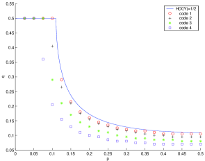
Figure 3: Feasible domain

V Conclusion

We have established an intimate connection between Slepian-Wolf coding and channel coding, which clarifies a misconception in the area of Slepian-Wolf code design. Interested readers may refer to [12] for more details.

References

- [1] D. Slepian and J. K. Wolf, “Noiseless coding of correlated information sources,” IEEE Trans. Inform. Theory, vol.IT-19, pp. 471-480, Jul. 1973.
- [2] S. S. Pradhan and K. Ramchandran, “Distributed source coding using syndromes (DISCUS): design and construction,” IEEE Trans. Inform. Theory, Mar. 2003.
- [3] T. P. Coleman, A. H. Lee, M. Mdard, and M. Effros, “Low-complexity approaches to Slepian-Wolf near-lossless distributed data compression,” IEEE Trans. on Inform. Theory, submitted for publication.
- [4] D. Schongberg, K. Ramchandran, and S. S. Pradhan, “Distributed code constructions for the entire Slepian-Wolf rate region for arbitrarily correlated sources,” Proceeding of IEEE Data Compression Conference (DCC), Snowbird, UT, Mar. 2004.
- [5] V. Stankovic, A. Liveris, Z. Xiong, and C. Georghiades, “On code design for the general Slepian-Wolf problem and for lossless multiterminal communication networks,” IEEE Trans. Inform. Theory, submitted for publication.
- [6] A. D. Wyner, “Recent results in Shannon theory,” IEEE Trans. Inform. Theory, vol. IT-20, pp. 2-10, Jan. 1974.
- [7] M. Luby, M. Mitzenmacher, A. Shokrollahi, D. Spielman, and V. Stemann, “Practical loss-resilient codes,” IEEE Trans. Inform. Theory, vol. 47, pp. 569-584, Feb. 2001.
- [8] T. Richardson and R. Urbanke, “The capacity of low-density paritycheck codes under message-passing decoding,” IEEE Trans. Inform. Theory, vol. 47, pp. 599-618, Feb. 2001.
- [9] T. Richardson, A. Shokrollahi, and R. Urbanke, “Design of capacity-approaching irregular low-density parity-check codes,” IEEE Trans. Inform. Theory, vol. 47, pp. 619-637, Feb. 2001.
- [10] J. Li, Z. Tu, and R. S. Blum, “Slepian-Wolf coding for nonuniform sources using Turbo codes,” Proceeding of IEEE Data Compression Conference (DCC), pp. 312-321, Snowbird, UT, March 2004.
- [11] S.-Y. Chung, “On the construction of some capacity-approaching coding schemes,” Ph.D. dissertation, Department of Electrical Engineering and Computer Science, MIT, 2000.
- [12] J. Chen, D.-k. He, and A. Jagmohan “Approaching the Slepian-Wolf limit with LDPC coset codes,” IEEE Trans. Inform. Theory, submitted for publication.