Weighted hierarchical alignment of
directed acyclic graphs

Abstract

In some applications of matching, the structural or hierarchical properties of the two graphs being aligned must be maintained. The hierarchical properties are induced by the direction of the edges in the two directed graphs. These structural relationships defined by the hierarchy in the graphs act as a constraint on the alignment. In this paper, we formalize the above problem as the weighted alignment between two directed acyclic graphs. We prove that this problem is NP–complete, show several upper bounds for approximating the solution, and finally introduce polynomial time algorithms for sub–classes of directed acyclic graphs.

1 The problem

Matching or alignment problems are an important set of theoretical problems that appear in many different applications [3, 4, 9]. Depending on the structure of the problem, polynomial time algorithms may or may not exist. In this paper, we propose a new type matching problem called the weighted hierarchical DAG (directed acyclic graph) alignment problem. In this problem, we have two directed acyclic graphs and a set of possible matchings between vertices in both graphs. We wish to find the maximum weighted matching between the vertices where the directed edges in both graphs act as hierarchical constraints on possible solutions to the matching. For example, if a vertex $v_{1}$ has a directed edge to a vertex $v_{2}$, then any matched vertex to $v_{2}$ cannot be an ancestor of $v_{1}$’s matched vertex (see Figures 1 and 2).

We became interested in this problem through our interest in ontology alignment. An ontology is a conceptualization of a domain [12]. This conceptualization consists of a set of terms with certain semantics and relationships [24]. Generally, the terms are related by $\verb"is_a"$ relationships. The relationships (edges) and terms (vertices) can be represented as a DAG. With ontology alignment, one wants to align terms from two different ontologies in order to merge, compare, or map the ontologies. Since the edges of the DAG represent an $\verb"is_a"$ relationship, then if we apply the strictist sense of this relationship, it constrains the number of valid matchings, because we do not wish to violate this relationship in the corresponding matching.

This type of hierarchical or structural constraint is important in other applications as well. The domains of SVG (Scalable Vector Graphics) version comparison, source code comparison/merging, UML difference calculation, and file/folder merging, are all instances of hierarchical based matching. For example, an SVG document is rich with structure. The document defines graphical objects, and how they relate, a form of the $\verb"is_a"$ relationship exists through the document graphic layers. In object–oriented programming, $\verb"is_a"$ relationships exist through the definitions of inheritance, and other relationships exist via class membership. Similarly, UML diagrams have structural relationships, and different versions of diagrams sometimes need to be merged or have their differences calculated for visual comparison [20]. Finally, in a file system, the folders represent an embedded hierarchy.

Figure 1: Example of a valid matching between two graphs. The dashed lines represent valid assignments for the vertices $A1,A2,A3,$ and $A4$.

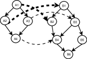
Figure 2: Example of an invalid matching between two graphs. The dashed lines represent the assignments for the vertices $A1,A2,A3,$ and $A4$. The two bold dashed lines represent an assignment violation because $A1$ maps to a descendant of $A2$’s mapped vertex $B1$.

1.1 Related work

General graph matching is a well studied problem. Most graph matching problems can be divided into two categories, graph isomorphisms and weighted graph matching. In graph isomorphism, the goal is to find a matching function $f$ for two graphs $G_{1}=(V_{1},E_{1})$ and $G_{2}=(V_{2},E_{2})$. General graph isomorphism is still open, that is, it is not known whether the problem is NP–hard or can be solved in polynomial time [10]. Sub–graph isomorphism is known to be NP–complete [11]. With weighted graph matching, we are given a graph $G=(V,E)$, where the edges have associated weights and we wish to find a subset $M$ of $E$, such that no two edges in $M$ share a common end vertex and such that the sum of edge weights in $M$ is maximum. For some classes of graphs, polynomial time algorithms are known, while some others are known to be NP–complete.

Both of these problems have many practical applications, in particular, graph isomorphism has received a lot of attention in the area of computer vision. Images or objects can be represented as a graph. A weighted graph can be used to formulate a structural description of an object [25]. There have been two main approaches to solving graph isomorphism: state–space construction with searching and nonlinear optimization. The first method consists of building the state–space, which can then be searched. This method has an exponential running time in the worst case scenario, but by employing heuristics, the search can be reduced to a low–order polynomial for many types of graphs [6, 26]. With the second approach (nonlinear optimization), the most successful approaches have been relaxation labeling [16], neural networks [19], linear programming [1], eigendecomposition [27], genetic algorithms [17], and Lagrangian relaxation [23].

Another type of graph problem related to ours is graph alignment through minimizing the edit distance [28, 5]. In this problem, the graphs are transformed via editing (deletion, insertion, relabelling) to achieve alignment. Our work is different is several ways. First, we do not allow any of the graph to be edited as is typically done in the edit distance problem. Second, in the work discussed in [28], the authors consider only undirected graphs as opposed to DAGs. Finally, the authors of [5] deal with unweighted alignment of trees as opposed to weighted alignment of DAGs.

As mentioned, we became interested in DAG alignment problem due to our interests in ontology alignment. Ontology alignment has recently received a lot of attention. An alignment between two ontologies can be formalized in terms of weighted graph matching, with certain constraints on the solution to any valid matching. Originally, alignments were performed by hand, and later, several researchers introduced semi–automatic alignment strategies, which make suggestions to the user about which terms to align [21, 22]. Since then, fully automatic alignment strategies have been explored. In [7], over twenty different tools/algorithms are discussed. Many of these approaches use heuristics to determine term similarities, by first comparing syntactic, semantic, and structural similarities, and then compute matches greedily or via some other local optimization technique.

In [8], graph matching is applied to conceptual system matching for translation. The work is very similar to ontology alignment, however, the authors formalize their problem in terms of any conceptual system rather than restricting the work specifically to an ontological formalization of a domain. They formalize conceptual systems as graphs, and introduce algorithms for matching both unweighted and weighted versions of these graphs.

1.2 Organization of the paper

The remainder of the paper is organized as follows. The next section introduces notations and definitions that will be used throughout the paper. The definitions include the formal description of the problem. Following this, we show that the decision version of the problem is NP–complete via a reduction from 3SAT. Next, we prove two theorems, which yield upper bounds on approximating the DAG alignment problem. After this, we introduce a polynomial time algorithm for trees and discuss its possible modifications. Finally, we present some concluding remarks, a short discussion of open problems, and directions for future research.

2 Notations and definitions

2.1 Notations

Before formally defining the DAG alignment problem we must first introduce some definitions. A DAG is a directed graph, $G=(V,E)$ that contains no oriented cycles, where $V$ is a set of vertices and $E$ is a set of edges. Let $anc(v)$ denote the set of ancestors for any $v\in V$, where an ancestor of $v$ is any $a\in V$ such that there exists a directed path from $a$ to $v$. Let $desc(v)$ denote the set of descendants for any $v\in V$, where a descendant of $v$ is any $d\in V$ such that there exists a directed path from $v$ to $d$. Finally, let $child(v)$ denote the set of direct children for any $v\in V$, where a direct child is any $d\in V$ such that there exists a directed edge from $v$ to $d$.

2.2 Description of problem

In this section we formalize the problem of DAG alignment with hierarchy constraints. Without the hierarchy constraint, the problem reduces to weighted bipartite matching, since the edges that represent vertex relationships would be ignored. As was mentioned, in many practical applications these structural relationships cannot be ignored. Due to these relationships, many solutions that would be valid in weighted bipartite matching are invalid. In fact, we can think of any edge $e$ as having a set of conflicting edges, where a conflict is any edge that would violate a matching solution that contained $e$. We formalize this in the following definition.

Definition 1

An edge conflict for edge $e=(a,b,w_{e})$, $w_{e}\in[0,1]$, is any edge $d=(f,g,w_{d})$, $w_{d}\in[0,1]$, and $d\neq e$, where one of the following conditions applies:

1. $a\in anc(f)$ and $b\not\in anc(g)$.

2. $a\in desc(f)$ and $b\not\in desc(g)$.

3. $a=f$.

4. $b=g$.

The set $conf(e)$ denotes the set of edges that have edge conflicts with edge $e$. We can now give the formal definition of the DAG alignment problem.

Definition 2

Given two DAGs, $G_{1}=(V_{1},E_{1})$ and $G_{2}=(V_{2},E_{2})$, and a set of edges $\beta=\{(v_{i},v_{j},w_{t})\}$ for all $v_{i}\in V_{1}$, all $v_{j}\in V_{2}$ and $w_{t}\in[0,1]$, the DAG alignment problem is to find the maximum weight matching, $M\subseteq\beta$, such that each vertex in $M$ appears only once and for any edge $e\in M$, $conf(e)\cap M=\emptyset$. We refer to this constraint on the matching as the hierarchical constraint for the remainder of this paper.

Our definition of the DAG alignment problem uses a complete bipartite graph of all possible matchings with the set of edges $\beta=\{(v_{i},v_{j},w_{t})\}$ defined for all $v_{i}\in V_{1}$ and all $v_{j}\in V_{2}$. This may appear to narrow the set of problems we are trying to solve, however, it does not. This is because a solution to the problem with an incomplete (some matchings may be inherently prohibitive) matching graph can be reduced to the problem with complete bipartite graph through the following consideration. Take a DAG alignment problem in which not every node of $G_{1}$ can potentially be mapped to any node of $G_{2}$. Allow all the remaining matchings, but assign zero weights to them. Solve the DAG alignment problem with the complete set of possible matchings. Delete all zero weight matchings from the solution. The result is a solution for the DAG alignment problem with incomplete set of possible matchings.

3 Intractability

The DAG alignment problem defined in the previous section is NP–complete. Before showing the proof of this, we begin by first defining the decision version of the problem.

Definition 3

We are given two DAGs, $G_{1}=(V_{1},E_{1})$ and $G_{2}=(V_{2},E_{2})$, and a set of edges $\beta=\{(v_{i},v_{j},w_{t})\}$ for all $v_{i}\in V_{1}$, $v_{j}\in V_{2}$ and $w_{t}\in[0,1]$. Let $w(A)$, where $A\subseteq\beta$, be the sum of all weights $w_{t}$ defined over all triples $(v_{i},v_{j},w_{t})\in A$. Is there a matching $M\subseteq\beta$ with weight $w(M)\geq X$ and $|M|\leq Y$ such that each vertex in $M$ appears only once and for any edge $e\in M$, $conf(e)\cap M=\emptyset$?

Theorem 3.1

DAG alignment, as introduced in Definition 3, is NP–complete.

Proof

It is easy to see that the decision version of DAG alignment is in NP, so this will be omitted.

We show a reduction of 3SAT to the decision version of the DAG alignment problem. In 3SAT we have a finite set of variables, $X=\{x_{1},x_{2},\ldots,x_{n}\}$ and a finite set of clauses $C=\{c_{1},c_{2},\ldots,c_{m}\}$, such that each clause is logic OR of 3 literals, where the literals over variable $x_{i}$ are $x^{0}_{i}$ ($:=x_{i}$) and $x^{1}_{i}$ ($:=\overline{x_{i}}$). The problem is to find a truth assignment to variables in $X$ such that the logic AND of all clauses in $C$ is satisfied.

Let $\phi=(X,C)$ be an instance of 3SAT. We can define an instance of the DAG alignment problem as follows. We begin by defining the two DAGs used in the alignment. First, let us define $G_{1}=(V_{1},E_{1})$ where $V_{1}$ is defined as follows

$$V_{1}=\bigcup_{c_{i}\in C}(x^{p1}_{j},i)\cup(x^{p2}_{k},i)\cup(x^{p3}_{l},i)\mbox{, where }$$

$$c_{i}=(x^{p1}_{j},x^{p2}_{k},x^{p3}_{l})\mbox{ and }p1,p2,p3\in\{0,1\}\mbox{ and }j,k,l\leq n.$$

We define the set of edges $E_{1}$ by creating directed edges over the vertices of $V_{1}$ as $((x^{0}_{j},i),(x^{1}_{j},t))$ for all $j\leq n$ and $i,t\leq m$.

Now, let us define a second DAG, $G_{2}=(V_{2},E_{2})$. First, we define $V_{2}$ as

$$V_{2}=\{\{y_{1},z_{1},y_{2},z_{2},\ldots y_{n},z_{n}\}\times\{1,2,\ldots,m\}\}$$

$$\bigcup\{\{c_{1},c_{2},\ldots,c_{m}\}\times\{1,2\}\}.$$

Intuition behind this definition is $y_{i}$ corresponds to $x_{i}$ and $z_{i}$ corresponds to $\overline{x_{i}}$.

We define $E_{2}$ by creating directed edges $((z_{j},i),(y_{j},t))$, $((y_{j},t),(c_{i},1))$ and $((y_{j},t),(c_{i},2))$ for all $j\leq n$ and $i,t\leq m.$

We now have two DAGs, $G_{1}$ and $G_{2}$. We must define the set $\beta$, which describes the possible matches between the two DAGs, and the related weights. For every vertex, $(x^{0}_{j},i)$ or $(x^{1}_{j},i)$, map this vertex to its corresponding vertex in $V_{2}$ with weight equal to one and add this to $\beta$. That is, $(x^{0}_{j},i)\in V_{1}$ maps to $(y_{j},i)\in V_{2}$ and $(x^{1}_{k},t)\in V_{1}$ maps to $(z_{k},t)\in V_{2}$, and so forth. Also, for each vertex $(x^{p}_{j},i)\in V_{1}$, create mappings $((x^{p}_{j},i),(c_{i},1))$ and $((x^{p}_{j},i),(c_{i},2))$ both with weight equal to one and add this to $\beta$. Let the total weight and the total number of vertices for the matching be $3m$.

We now show that the DAG alignment problem, as described above, has a matching satisfying the hierarchical mapping constraint, if and only if $\phi$ is satisfiable.

($\Rightarrow$) Assume $\phi$ is satisfiable. For each clause $c_{i}$, choose a single literal $x^{p}_{j}$. If variable $x_{j}\in X$ is true and $p=0$ or $x_{j}\in X$ is false and $p=1$, then include edge $((x^{0}_{j},i),(y_{j},i))$ in the matching $M$. Also, for any clause $c_{t}$ with $x^{1}_{j}$ include edge $((x^{1}_{j},t),(c_{t},1))$ if vertex $(c_{t},1)$ is not in the matching, otherwise include edge $((x^{1}_{j},t),(c_{t},2))$. Similarly, if variable $x_{j}\in X$ is true and $p=1$ or $x_{j}\in X$ is false and $p=0$, then include $((x^{1}_{j},i),(z_{j},i))$ in the matching. Also, for any clause $c_{t}$ with $x^{0}_{j}$, include edge $((x^{0}_{j},t),(c_{t},1))$ if vertex $(c_{t},1)$ is not in the matching, otherwise include edge $((x^{0}_{j},t),(c_{t},2))$. Thus, $M$ exactly maps all vertices in $G_{1}$ to vertices in $G_{2}$. There are $3m$ vertices in $V_{1}$, so $|M|=3m$. Also, since the weight of each edge is one, $w(M)=3m$. Finally, since both $x^{0}_{j}$ and $x^{1}_{j}$ cannot be true, both edges $((x^{0}_{j},i),(y_{j},i))$ and $((x^{1}_{j},i),(z_{j},i))$ cannot be in $M$, therefore the hierarchical constraint is satisfied.

($\Leftarrow$) Let $M$ be a solution to the DAG alignment problem. The truth value of any variable $x_{j}$ is assigned as follows. If, for any clause $c_{i}$ with literal $x^{0}_{j}$, there exists an edge $((x^{0}_{j},i),(y_{j},i))$ from $G_{1}$ to $G_{2}$, then let $x_{j}$ be true. Similarly, if there exists an edge $((x^{1}_{j},i),(z_{j},i))$ from $G_{1}$ to $G_{2}$, then let $x_{j}$ be false. Since in $G_{1}$, every vertex $(x^{0}_{j},i)$ has an edge to every $(x^{1}_{j},t)$, and in $G_{2}$ every vertex $(z_{j},i)$ has an edge to every $(y_{j},t)$, $M$ cannot contain edges $((x^{0}_{j},i),(y_{j},i))$ and $((x^{1}_{j},i),(z_{j},i))$, otherwise the hierarchical constraint would be violated. Thus, $x^{0}_{j}$ or $x^{1}_{j}$ is true, but never both. Also, since any false literal in a clause $c_{i}$ is mapped to a vertex $(c_{i},1)$ or $(c_{i},2)$, at most 2 vertices in any clause can be false. Thus, $\phi$ is satisfied.

4 Upper bounds on approximating weighted DAG alignment

Since weighted DAG alignment belongs to the class of NP–complete problems, it is unlikely that we will find a polynomial time solution to the problem. Thus, we must rely on an approximation scheme for computing alignments.

In this section, we introduce two polynomial time reductions of the DAG alignment problem to other known NP–complete problems and use these to provide upper bounds for approximating the weighted DAG alignment problem. The quality of the approximation is given as the ratio between the size of the maximum weighted DAG alignment and the approximation found. The ratio in the worst–case scenario defines the performance guarantee of the algorithm.

We begin by reducing the DAG alignment problem to Weighted Independent Set (WIS). In the Independent Set problem, we are given a graph $G=(V,E)$, and we wish to find the largest subset $S\subseteq V$, such that no two vertices in $S$ are connected by an edge in $E$. In the weighted version of this problem, each node, $v_{i}\in V$, has an associated weight $w_{i}$, and we wish to find the maximum weighted independent set.

Håstad [13] showed that Independent Set is hard to approximate within $n^{1-\epsilon}$, for $\epsilon>0$, unless NP–hard problems have randomized polynomial time solutions. In [2], Boppana and Halldórsson introduced the Ramsey algorithm for solving WIS. The algorithm is an extension of the naive greedy approach, where in the greedy approach a vertex $v$ is arbitrarily selected from the graph and added to the independent set, all adjacent vertices are removed, and this process is continued until all vertices are exhausted. The obvious problem with this solution is that the adjacencies are ignored. The first extension to this process is to consider not only the vertex $v$, but also the neighbors of $v$. The algorithm recurses by first considering $v$ as part of the independent set, and then $v$ not in the independent set, and selecting the better of the two results. This algorithm performs well provided the maximum Clique size is small. Boppana and Halldórsson further extended this algorithm by first removing the maximum set of disjoint $k$–cliques, and then apply the Ramsey algorithm to compute the independent set on this modified graph. From this, they were able to prove that the algorithm had a performance guarantee of $O(n/\log^{2}n)$, where $n$ is the number of vertices in the graph.

The following shows that any instance of the DAG alignment problem can be reduced, in polynomial time, to an instance of WIS. This reduction will allow us to use approximation strategies for Independent Set to find approximate solutions to the DAG alignment problem.

Theorem 4.1

The ontology alignment problem can be approximated within $O(m/log^{2}m)$ where $m=|\beta|$.

Proof

Consider an instance of the DAG alignment problem, defined by graphs $G_{1}=(V_{1},E_{1})$ and $G_{2}=(V_{2},E_{2})$, and the set of edges $\beta$. We define an instance of WIS, by constructing a graph $G=(V,E)$ as follows. For each edge $e=(a,b,w_{e})\in\beta$, construct a corresponding $v\in V$, and let the weight of vertex $v$ be $w:=w_{e}$. Next, let $E=\{(v_{i},v_{j})|e_{j}\in conf(e_{i})\mbox{ and }e_{i},e_{j}\in\beta\}$.

Now, we claim that a solution to WIS, defined over graph $G$, corresponds to a solution to the DAG alignment problem. We construct this solution as follows. Let $S$ be our solution to WIS. Then, for each $v_{i}\in S$, add the edge from $\beta$ that corresponds to $v_{i}$, to our DAG alignment solution $M$. This precisely constructs a valid DAG alignment, since each $v_{i}\in S$ cannot be connected to any other $v_{j}\in S$, which implies that for edges $e_{i},e_{j}\in M$, $e_{i}\not\in conf(e_{j})$. Since no edges in $M$ conflict, this must be a valid solution.

WIS can be approximated within $O(n/log^{2}n)$, where $n$ is the number of vertices in the graph. In our reduction, $n$ corresponds to $|\beta|$, by letting $m=|\beta|$, we achieve an approximation of $O(m/log^{2}m)$.

Next, we improve this bound via a reduction to the Weighted Set Packing (WSP) problem. In WSP, we have a set $S$ of $m$ base elements, and a collection $\mathcal{U}=\{U_{1},U_{2},\ldots,U_{n}\}$ of weighted subsets of $S$. We want to find a subcollection $\mathcal{U}^{\prime}\subseteq\mathcal{U}$ of disjoint sets of maximum total weight.

In [15], an approximation guarantee of $\sqrt{m}$, where $m=|S|$ is given for WSP. The algorithm is based on a variant of the greedy algorithm for solving the non-weighted version introduced in [14]. In the following theorem, we show that any instance of the DAG alignment problem can be reduced to WSP in polynomial time, and that a solution to WSP corresponds to a solution of the DAG alignment problem.

Theorem 4.2

The DAG alignment problem can be approximated within $\sqrt{m}$ where $m=|\beta|$.

Proof

Consider an instance of the DAG alignment problem, defined by graphs $G_{1}=(V_{1},E_{1})$ and $G_{2}=(V_{2},E_{2})$, and the set of edges $\beta$. We define an instance of WSP, by constructing $S$ and the collection $\mathcal{U}$ as follows.

We let our $m$ base elements be the edges specified by $\beta$, thus our set $S=\beta$. We construct the collection $\mathcal{U}$, by defining subsets $U_{i}$ for all $e_{i}\in\beta$ as $U_{i}=\{\{e_{i}\}\bigcup conf(e_{i})\}$. Let the weight of $U_{i}$ be equal to $w_{e_{i}}$. We now claim that any solution to WSP, $\mathcal{U}^{\prime}$, corresponds to a solution the DAG alignment problem.

We can see this by considering any $\mathcal{U}^{\prime}$. We construct a solution to the DAG alignment problem by taking each $U_{i}\in\mathcal{U}^{\prime}$, and adding edge $e_{i}\in\beta$ to our ontology alignment solution $M$. This is a valid matching because every $U_{i}\in\mathcal{U}^{\prime}$ is disjoint, which implies that for each $e_{i}\in M$ and $e_{j}\in M$, $e_{i}\not\in conf(e_{j})$, so no edges in $M$ conflict.

Since a solution to WSP yields a solution to the DAG alignment problem, approximations of WSP correspond to approximations of the DAG alignment problem. Hence, we can approximate the DAG alignment problem within $\sqrt{m}$, where $m=|\beta|$.

5 Polynomial-time algorithms

In this section we study certain types/classes of graphs with respect to their DAG alignment problem solution complexity. In particular, we show that the DAG alignment problem for trees has a polynomial time solution. In this work, we naturally define trees to be those directed trees with all edges directed away from a particular vertex called the root. In this section we show that any two such trees can be aligned in polynomial time. Furthermore, a chain $C_{n}$ is defined as a DAG with $n$ vertices $v_{1},v_{2},...,v_{n}$ and directed edges $(v_{1},v_{2}),\;(v_{2},v_{3}),...\;,(v_{n-1},v_{n})$.

Theorem 5.1

Any two trees can be aligned in polynomial time.

Proof

We first describe the data structure used in our algorithm, and then explain how it can be used to achieve a polynomial time algorithm that aligns two trees. Our algorithm is a form of bottom-up approach that applies weighted bipartite matching at each of $n\times k$ iterations it makes.

Suppose we have two trees $T^{1}=(V^{1},E^{1})$ and $T^{2}=(V^{2},E^{2})$ with $n$ and $k$ vertices correspondingly that need to be aligned. Create an array with $n\times k$ empty cells $C(i,j)\;(i=1..n,j=1..k)$ that contain real numbers whose values will be assigned during the algorithm and will hold values for best alignment of the subtree of $T^{1}$ with root in $v^{1}_{i}$ with the subtree of $T^{2}$ with root in $v^{2}_{j}$. This array is complemented by an equal size array $M(i,j)\;(i=1..n,j=1..k)$ that contains the actual matchings used for the assigned values of $C(i,j)$. We will further describe how to assign values to $C(i,j)$, sometimes omitting the discussion of updates to $M(i,j)$. Our algorithm terminates when $C(n,k)$ gets assigned a value. Once this is done, the value stored in $C(n,k)$ equals to the maximum weight alignment and $M(n,k)$ contains the best matching.

We next describe the total order on the set of vertices of both trees and order cells $C(i,j)$. Consider tree $T^{1}$. Suppose its depth is $d$. Name all vertices at level $d$, $v^{1}_{1}$ through $v^{1}_{d_{1}}$ (for instance, name these vertices in the left to right order assuming the tree is drawn on paper with no edge intersections) for appropriate value of $d_{1}$. Next, name all depth $d-1$ vertices, $v^{1}_{d_{1}+1}$ through $v^{1}_{d_{2}}$, for appropriate value $d_{2}$. Continue this operation until all vertices are named. Vertex $v^{1}_{n}$ is thus the root of tree $T^{1}$. Apply the same method to enumerate vertices in tree $T^{2}$. Cells $C(i,j)$ are ordered lexicographically, e.g. $C(1,1)\prec C(1,2)\prec...\prec C(1,k)\prec C(2,1)\prec C(2,2)\prec...\prec C(n,k)$. We fill values $C(i,j)$ (and keep track of alignment made by updating $M(i,j)$) in this order.

$C(1,1)$ is easy to find, because it is equal to the weight of edge $e=(v^{1}_{1},v^{2}_{1},w_{e})$ of the matching problem. To find the value of $C(i,j)$ (and update $M(i,j)$) consider the following cases (with $C(i,j)$ taking the maximal value among those found in each of the cases below):

1. $v^{1}_{i}$ does not get mapped anywhere. In this case, $C(i,j)=\max\{C(v^{1}_{t},v^{2}_{j})|v^{1}_{t}=child(v^{1}_{i})\}$. Each such $C(v^{1}_{t},v^{2}_{j})\prec C(i,j)$ and thus the maximum, is well defined and can be calculated. The computational cost of this calculation is the number of children of $v^{1}_{i}$, i.e. no more than $n$.

2. $v^{1}_{i}$ is mapped to $v^{2}_{k}\in desc(v^{2}_{j})$, and hence $k<j$. In this case, $C(i,j)=w(v^{1}_{i},v^{2}_{k})+S$, where $S$ is the answer to the following weighted bipartite matching problem. Assuming $v^{1}_{i}$ has children $child^{1}_{1},child^{1}_{2},...,child^{1}_{ic}$ and $v^{2}_{k}$ has children $child^{2}_{1},child^{2}_{2},...,child^{2}_{kc}$, the maximum bipartite matching problem whose solution is the number $S$ we are interested in is defined for the complete bipartite graph with vertices $child^{1}_{1},child^{1}_{2},...,child^{1}_{ic},child^{2}_{1},child^{2}_{2},$ $...,child^{2}_{kc}$ and edges with weights $C(child^{1}_{s},child^{2}_{t})|_{s=1..ic,t=1..kc}.$ Note that all such weights are known and thus the problem is well defined. The solution to the maximum weighted bipartite matching can be found in polynomial time, and the number of times we call for a solution is limited by the number of descendants of $v^{2}_{j}$, which is never more than $k$ (the number of vertices in tree $T^{2}$). Thus, this step can be completed in polynomial time.

The number of different $C(i,j)$ is polynomial, and the amount of work required to fill in each value is polynomial. Thus, our algorithm is polytime. For two trees with $n$ vertices each, the complexity of our algorithm is $O(n^{6})$: there are $n^{2}$ numbers $C(i,j)$ to calculate, and calculation of each requires (item 2) at most $n\times n^{3}$ operations assuming the Hungarian algorithm [18] for weighted bipartite matching is used.

It appears that the complexity of the DAG alignment problem moves from P to NP–complete in transition from trees to DAGs. The part of the above proof that works for trees and breaks for DAGs is the ability to establish an order on the numbers $C(i,j)$ such that once a particular $C(i,j)$ has been calculated it never needs to get updated.

The described polynomial time algorithm requires $O(n^{6})$ runtime to align two trees. However, for some simpler types of trees the polynomial time complexity can be reduced through considering simplified and modified versions of the above algorithm. A detailed description of such algorithms is out of scope for this paper. However, we would like to mention that two chains (with $n$ vertices each) can be aligned with a cost of $O(n^{3})$ and two complete binary trees with the cost of $O(\frac{n^{4}}{\log(n)})$.

6 Conclusions

We introduced a new type of weighted matching problem called the weighted hierarchical DAG alignment problem. We formalized this problem, showed that it is NP–complete, proved several upper bounds for approximating solutions to the problem, and finally introduced algorithms for solving different classes of the problem. This problem developed through our research on ontology alignment, however, it relates to many different applications, including, but not limited to, UML diagram comparison, SVG document comparison, and file/folder mapping. Our results show that, in particular, file/folder mapping problem can be solved in polynomial time, since the underlying data structure is a tree.

In the future, we plan to find other classes of DAGs that can be aligned faster than with an exponential time algorithm, work on designing efficient heuristics, and finally apply some of these ideas to the problem of aligning ontologies.

With ontologies, the problem becomes even more complex because they can contain errors in their specification, meaning that in some circumstances the hierarchical constraint must be relaxed. Moreover, this is likely the case with other applications of the problem. Thus, it may also be an interesting problem to investigate approximate solutions that are allowed to contain a small number of edge conflicts, which will accommodate for some human error in an ontology specification.

References

- [1] H. A. Almohamad and S. O. Duffuaa. A linear programming approach for the weighted graph matching problem. IEEE Transactions on Pattern Analysis and Machine Intelligence, 15(5):522–525, 1993.
- [2] R. Boppana and M. M. Halldórsson. Approximating maximum independent sets by excluding subgraphs. In J. R. Gilbert and R. Karlsson, editors, SWAT 90 2nd Scandinavian Workshop on Algorithm Theory, volume 447, pages 13–25, 1990.
- [3] S. Buss and P. Yianilos. A bipartite matching approach to approximate string comparison and search. Technical report, 1995.
- [4] Yves Caseau and Francois Laburthe. Solving various weighted matching problems with constraints. In Principles and Practice of Constraint Programming, pages 17–31, 1997.
- [5] E. D. Demaine, S. Mozes, B. Rossman, and O. Weimann. An o(n^3)-time algorithm for tree edit distance. http://arxiv.org/abs/cs.DS/0604037, April 2006.
- [6] M. A. Eshera and K. S. Fu. A graph distance measure for image analysis. IEEE Transactions on Systems, Man, and Cybernetics, 14(3):398–408, 1984.
- [7] J. Euzenat, T. Le Bach, J. Barrasa, P. Bouquet, J. DeBo, R. Dieng-Kuntz, M. Ehrig, M. Hauswirth, M. Jarrar, R. Lara, D. Maynard, A. Napoli, G. Stamou, H. Stuckenschmidt, P. Shvaiko, S. Tessaris, S. Van Acker, and I. Zaihrayeu. State of the art on ontology. deliverable d2.2.3, 2004.
- [8] Y. Feng, R. L. Goldstone, and V. Menkov. A graph matching algorithm and its application to conceptual system translation. International Journal on Artificial Intelligence Tools, 14:77–100, 2005.
- [9] Z. Galil, S. Micali, and H. Gabow. An algorithm for finding a maximal weighted matching in general graphs. SIAM J. Comput., 15(1):120–130, 1986.
- [10] M. R. Garey and D. S. Johnson. Computers and Intractability : A Guide to the Theory of NP-Completeness. W. H. Freeman, 1979.
- [11] S. Gold and A. Rangarajan. A graduated assignment algorithm for graph matching. IEEE Transactions on Pattern Analysis and Machine Intelligence, 18(4):377–388, 1996.
- [12] T. R. Gruber. A translation approach to portable ontology specifications. Knowledge Acquisition, 5(2):23–28, 1993.
- [13] J. Håstad. Clique is hard to approximate within . Acta Mathematica, 182:105–142, 1999.
- [14] M. Halldórsson, J. Kratochvil, and J. Telle. Independent sets with domination constraints. Discrete Applied Mathematics, 99:39–54, 1999.
- [15] M. M. Halldórsson. Approximation of weighted independent set and hereditary subset problems. In Proceedings of COCOON’99, 1999.
- [16] R. A. Hummel and S. W. Zucker. On the foundations of relaxation labeling processes. IEEE Transactions on Pattern Analysis and Machine Intelligence, 5(3), 1983.
- [17] M. Krcmar and A. Dhawan. Application of genetic algorithms in graph matching. In International Conference on Neural Networks, volume 6, pages 3872–3876, 1994.
- [18] H. W. Kuhn. The hungarian method for the assignment problem. Naval Research Logistics Quaterly, 2:83–95, 1955.
- [19] P. Kuner and B. Ueberreiter. Pattern recognition by graph matching combinatorial versus continuous optimization. International Journal Pattern Recognition and Artificial Intelligence, 2:527–542, 1988.
- [20] J. Niere. Visualizing differences of uml diagrams with fujaba. In Proceedings of the Fujaba Days 2004, 2004.
- [21] N. Noy and M. Musen. The prompt suite: Interactive tools for ontology merging and mapping. Technical report, 2002.
- [22] N. F. Noy and M. A. Musen. An algorithm for merging and aligning ontologies: Automation and tool support. In Sixteenth National Conference on Artificial Intelligence (AAAI-99), Workshop on Ontology Management, 1999.
- [23] A. Rangarajan and E. Mjolsness. A Lagrangian relaxation network for graph matching. In International Conference on Neural Networks, volume 7, pages 4629–4634. Inst. Electrical & Electronics Engineers, 1994.
- [24] S. Russell and P. Norvig. Artificial Intelligence: A Modern Approach. Prentice Hall, Upper Saddle River, New Jersey, 1995.
- [25] L. Shapiro and R. Haralick. Structural descriptions and inexact matching. IEEE Transactions on Pattern Analysis and Machine Intelligence, 3:504–519, 1981.
- [26] W. H. Tsai and K. S. Fu. Subgraph error-correcting isomorphism for syntactic pattern recognition. IEEE Transactions on Systems, Man and Cybernetics, 13:48–62, 1983.
- [27] S. Umeyama. An eigendecomposition approach to weighted graph matching problems. IEEE Transactions on Pattern Analysis and Machine Intelligence, 10(5):695–703, 1988.
- [28] K. Zhang, J. T. L. Wang, and D. Shasha. On the editing distance between undirected acyclic graphs and related problems. In Proceedings of the 6th Annual Symposium on Combinatorial Pattern Matching, volume 937, pages 395–407. Springer-Verlag, 1995.