On symmetric sandpiles

Abstract

A symmetric version of the well-known SPM model for sandpiles is introduced. We prove that the new model has fixed point dynamics. Although there might be several fixed points, a precise description of the fixed points is given. Moreover, we provide a simple closed formula for counting the number of fixed points originated by initial conditions made of a single column of grains.

Keywords:  SOC systems; sandpiles; fixed point dynamics; discrete dynamical systems.

1 Introduction

Self-Organized Criticality (SOC) is a very common phenomenon which can be observed in Nature. It concerns, for example, sandpiles formation, snow avalanches and so on [1].

Practically speaking, it can be described as follows. Consider an evolving system. After a while, the system reaches a critical state. Any further move from this critical state will cause a deep spontaneous reorganization of the whole system. No external parameter can be tuned to control this reorganization. Thereafter, the system starts evolving to another critical state and so on.

Sandpiles are a very useful model to illustrate SOC systems. Indeed, consider toppling sand grains on a table, one by one. Little by little a sandpile will start growing and growing until the slope reaches a critical value. At this moment, any further addition of a single sand grain will cause cascades of grains and deep reorganization of the whole pile. Afterwards the sandpile restarts growing to another critical state and so on.

A formal model for sandpiles, called SPM, has been introduced in [6, 7, 8]. The sandpile is represented by a sequence of “columns”. Each column contains a certain number of sand grains. The evolution is based on a local interaction rule (see Section 2): a sand grain falls from a column $A$ to its right neighbor $B$ if $A$ contains at least two grains more than $B$; otherwise there is no movement. The SPM model has been widely studied [2, 6, 11, 3, 10, 9]. In particular, it has been proved that it has fixed point dynamics and a closed formula has been given to calculate precisely the length of the transient to the fixed point [6]. Moreover, a precise description of the fixed point has been given [7].

All these results are very interesting but they have two main drawbacks. First, they lack generality; indeed, the fixed point results are always obtained starting from very special initial sandpiles (just one column). In [5, 4], we tried to solve this problem by giving a fast algorithm for finding the fixed point starting from any possible initial condition. Second, the model lacks symmetry; in fact, grains either stay or move to the right only. Remark that in Nature, sandpiles evolve absolutely in a symmetrical manner.

In this paper we introduce SSPM: a symmetric version of SPM. The new model follows the rules of SPM but it applies them in both directions. For technical reasons that will be clearer later, we allow only one grain to move per time step.

We prove that SSPM has fixed point dynamics. This is not a great surprise. To validate the new model, one should give a precise description of these fixed points and compare their “shape” with those of sandpiles in Nature.

To this extent we use a formal construct which allows a better description of the dynamics: orbit graphs. They are directed graphs of the relation “being son of”. In Section 3.2, the precise structure of their vertices is given (under the condition of considering initial configurations made by a single column): a configuration belongs to some orbit graph if and only if it admits a crazed LR-decomposition (see Section 3.2).

Practically speaking, a configuration admits a crazed LR-decomposition if it can be decomposed into an increasing part $L$ and a decreasing part $R$ and both in $L$ and in $R$ any two plateaus (i.e. consecutive columns of identical height) are separated by at least a “cliff” (i.e. consecutive columns with height difference strictly greater than $1$).

The special structure of the vertices allows a very useful description of the fixed points: they are configurations which admit a crazed LR-decomposition without cliffs.

Finally, using this characterization of the “shape” of fixed points we provide a closed formula which computes the number of fixed points originated from the initial configuration $(n)$ (a single column containing $n$ grains). The surprise is that the formula is $\lfloor\sqrt{n}\rfloor$. Unfortunately, we have no practical or “visual” explanation for such a formula.

2 The SPM model

A sandpile is a finite sequence of integers $(c_{1},\ldots,c_{k})$; $k\in\mathbb{N}$ is the length of the pile. Sometimes a sandpile is also called a configuration. Let $\mathcal{C}=\bigcup_{k\in\mathbb{N}}(\mathbb{N}^{+})^{k}$ be the set of all configurations.

Given a sandpile $(c_{1},\ldots,c_{k})$, the integer $n=\sum_{i=1}^{k}c_{i}$ is the number of grains of the pile. Given a configuration $(c_{1},\ldots,c_{k})$, a subsequence $c_{i},\dots,c_{j}$ (with $1\leq i<j\leq k$) is a plateau if $c_{h}=c_{h+1}$ for $i\leq h<j$; $s=i-j+1$ is the length of the plateau and $p=c_{i}$ its height. A subsequence $c_{i},c_{i+1}$ is a cliff if $c_{i}-c_{i+1}\geq 2$.

In the sequel, each sandpile $(c_{1},\ldots,c_{k})$ will be conveniently represented on a two dimensional grid where $c_{i}$ is the grain content of column $i$.

A sandpile system is a finite set of rules that tell how the sandpile is updated. SPM [6] (Sand Pile Model) is the most known and the most simple sandpile system. All initial configurations contain $n$ grains in the first column and nothing elsewhere i.e. they are of type $(n)$. It consists in only one local rule which moves a grain to the right whenever there is a cliff (see Figure 1).

Figure 1: local rule of SPM.

Formally, for any configuration $c$, if there exists $i\in\mathbb{N}$ such that $c_{i}-c_{i+1}\geq 2$, then $c$ evolves to $c^{\prime}$ according the following relations:

$$\left\{\begin{array}[]{rcl}c^{\prime}_{i}&=&c_{i}-1\\ c^{\prime}_{i+1}&=&c_{i+1}+1\enspace.\\ \end{array}\right.$$

This process is iterated until the rule cannot be applied anymore. We say that a fixed point is reached.

Along the evolution of the pile, the rule may be applicable at different places in the configuration. To illustrate this, we represent the set of reachable configurations (starting from a single column) on an oriented graph where the vertices are the configurations. There is an edge between two configurations $c^{1}$ and $c^{2}$ when $c^{2}$ can be obtained by applying the local rule somewhere in $c^{1}$ (see Figure 2 for an example, starting from a single column with 8 grains). This is called the orbit graph of the initial configuration $c$, denoted by $\mathcal{G}_{c}$.

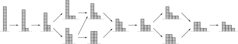
Figure 2: $\mathcal{G}_{(8)}$, orbit graph of a single pile with $8$ grains for SPM.

The following theorem proves that the fixed point is unique, independently of the order of application of the local rule.

Theorem 1 ([6]).

For any integer $n$, $\mathcal{G}_{(n)}$ for SPM is a lattice and is finite.

The following lemma characterizes the elements of the lattice.

Lemma 2 ([7]).

Consider a configuration $c$ and let $n$ be its number of grains. Then, $c\in\mathcal{G}_{(n)}$ for SPM if and only if it is decreasing and between any two plateaus of $c$ there is at least a cliff.

Remark 1.

Consider a configuration $c$, and assume that $c$ contains a plateau of length $3$. Such a plateau can be seen as two consecutive plateaus of length $2$. Thus, by Lemma 2, $c$ does not belong to any orbit graph.

From Lemma 2, it is easy to see that a fixed point $\Pi$ is a decreasing configuration with no cliffs and at most one plateau. Therefore for any $n\in\mathbb{N}$, we can describe the fixed point $\Pi$ of $(n)$ by

$$\Pi=\left\{\begin{array}[]{l@{\hspace{1cm}}l}(p,p-1,\ldots,1)\hfil\hskip 28.45274pt&\text{if $q=0$}\enspace,\\ (p,p-1,\ldots,q+1,q,q,q-1,\ldots,1)\hfil\hskip 28.45274pt&\text{otherwise,}\end{array}\right.$$

where $\langle p,q\rangle$ is the unique decomposition of $n$ in its integer sum:

$$n=q+\sum_{i=1}^{p}i=q+\frac{p\cdot(p+1)}{2}\enspace.$$

3 The symmetric model

In this section we extend SPM to SSPM (Symmetric SPM) according to the following guidelines:

• a grain can move either to the left or to the right, if the difference is more than $2$;

• when a grain can move only in one direction, it follows the SPM rule (right) or its symmetric (left).

For all configurations $c=(c_{1},\ldots,c_{k})$, the following local rules formalize the above requirements:

$$V^{r}_{i}(c_{1},\ldots,c_{k})=\begin{cases}(c_{1},\ldots,c_{i}\mathbf{-1},c_{i+1}\mathbf{+1},\ldots,c_{k})&\text{if}\;i\neq k\enspace,\\ (c_{1},\ldots,c_{k}\mathbf{-1},\mathbf{1})&\text{otherwise},\\ \end{cases}$$

$$V^{l}_{i}(c_{1},\ldots,c_{k})=\begin{cases}(c_{1},\ldots,c_{i-1}\mathbf{+1},c_{i}\mathbf{-1},\ldots,c_{k})&\text{if}\;i\neq 1\enspace,\\ (\mathbf{1},c_{1}\mathbf{-1},\ldots,c_{k})&\text{otherwise.}\\ \end{cases}$$

Let $\delta^{r}_{i}(c)$ denote the difference between the grain content of column $i$ and the one of column $i+1$ of $c$; define $\delta^{r}_{k}(c)=c_{k}$. Similarly, $\delta^{l}_{i}(c)$ denotes the difference between the grain content of column $i$ and the one of column $i-1$ of $c$ with $\delta^{l}_{1}(c)=c_{1}$.

Notation.

For $a,b\in\mathbb{N}$ with $a<b$, let $[a,b]$ denote the set of integers between $a$ and $b$.

From the local rule we can define a next step rule $\bar{f}:\mathcal{C}\mapsto\mathfrak{P}(\mathcal{C})$ as follows

$$\bar{f}\left(c\right)=\big{\{}V^{r}_{i}(c)\;|\;\delta^{r}_{i}(c)\geq 2,i\in[1,k]\big{\}}\cup\big{\{}V^{l}_{i}(c)\;|\;\delta^{l}_{i}(c)\geq 2,i\in[1,k]\big{\}}\enspace.$$

Finally, using the next step rule, one can define the global rule which describes the evolution of the system from time step $t$ to time step $t+1$ :

$$\forall S\in\mathfrak{P}(\mathcal{C}),\;f(S)=\bigcup_{c\in S}\bar{f}\left(c\right)\enspace.$$

When no local rule is applicable to $c$, i.e. $f(\{c\})=\emptyset$, we say that $c$ is a fixed point of SSPM. For $n\in\mathbb{N}$, let $f^{n}$ denote the $n$-th composition of $f$ with itself.

The notion of orbit graph can be naturally extended to the symmetric case by using the functions $V^{r}_{i}$ and $V^{l}_{i}$. In the sequel, when speaking of orbit graph, we will always mean the orbit graph w.r.t. the SSPM model.

3.1 Fixed point dynamics

In this section we prove that SSPM has fixed points dynamics. This result is obtained by using a “potential energy function” and by showing that this function is positive and non-increasing.

Given a configuration $c=(c_{1},\ldots,c_{k})$, the energy of a column $c_{i}$ ($i\in[1,k]$) is defined as follows

$$\varepsilon(c_{i})=\sum_{j=1}^{c_{i}}j\enspace.$$

Therefore, the total energy of a configuration $c=(c_{1},\ldots,c_{k})$ is naturally defined as

$$E(c)=\sum_{i=1}^{k}\varepsilon(c_{i})\enspace.$$

Lemma 3.

Consider a configuration $c=(c_{1},\ldots,c_{k})$ with $n$ grains. Then it holds that $E(c)\leq E((n))$; equality holds if and only if $c=(n)$.

Proof.

Remark that $n=\sum_{i=1}^{k}c_{i}$. Define $h(i)=\sum_{j=c_{1}+c_{2}+\cdots+c_{i-1}+1}^{c_{1}+c_{2}+\cdots+c_{i}}j$. Then, $E((n))=\sum_{j=1}^{n}j$ can be rewritten as $E((n))=\sum_{i=1}^{k}h(i)$. Note that $h(i)\geq\epsilon(c_{i})$ for any $i\in[1,k]$; equality holds if and only if $i=1$. ∎

The function $E$ can be naturally extended to work on set of configurations as follows

$$\forall S\in\mathfrak{P}(\mathcal{C}),\;E(S)=\max\left\{E(c),\,c\in S\right\}\enspace,$$

with $E(\emptyset)=0$.

The following lemma is straightforward from the definition of the energy function.

Lemma 4.

For any set of configurations $S\neq\emptyset$, $E(f(S))<E(S)$.

The following simple proposition describes the general structure of the orbit graph.

Proposition 5.

For any initial configuration $c$, $\mathcal{G}_{c}$ is finite, contains at least a fixed point but no cycles.

Proof.

If $\bar{f}\left(c\right)=\emptyset$ i.e. c is a fixed point, then we are done. Assume that $c$ is not a fixed point. Remark that its energy is finite. By Lemma 4, it holds that $E(\left\{c\right\})>E(f(\left\{c\right\}))$ and $E(f^{t}(\left\{c\right\}))>E(f^{t+1}(\left\{c\right\}))$ for $t>1$ (unless $f^{t}(\left\{c\right\})=\emptyset$). Since $E$ is a positive function, there must exist $h\in\mathbb{N}$ such that $f^{h}(\left\{c\right\})=\emptyset$. Then, $f^{h-1}(\left\{c\right\})$ contains a fixed point. If $f^{h}(\left\{c\right\})=\emptyset$, then the orbit graph $\mathcal{G}_{c}$ is finite, since $|f^{t}(\left\{c\right\})|$ is finite for any $t\in\mathbb{N}$.

Finally, there are no cycles in $\mathcal{G}_{c}$ otherwise the elements of the cycle would contradict Lemma 4. ∎

The following corollary is given only to further stress the result of Proposition 5.

Corollary 6.

SSPM has fixed point dynamics.

Corollary 6 says that independently of the order of application of local rules both with respect to type of rule and to the application site, SSPM evolves towards a fixed point. The problem is that this fixed point might not be unique. Figure 3 gives an example of this fact.

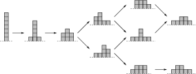
Figure 3: $\mathcal{G}_{(5)}$, orbit graph of a single pile with $5$ grains for SSPM. Remark that there are two distinct fixed points.

Despite the non-uniqueness, in the next section we give a precise characterization of the structure of the fixed points. This characterization is essentially deduced from the properties of the vertices of the orbit graphs.

3.2 Orbit graphs

In [7], the authors precisely described the structure of the orbit graph of SPM when started on initial condition $(n)$. They proved that it is the graph of a lattice. As a consequence, they deduced the uniqueness of the fixed point for SPM.

We have already seen that in the SSPM case, the dynamics is of fixed point type, but the fixed point might not be unique. Hence, it is clear that the orbit graph of SSPM is no more the graph of a lattice. In this section, we detail the overall structure of the vertices of these graphs.

A configuration $c=(c_{1},c_{2},\ldots,c_{k})$ is LR-decomposable if it can be divided into two zones: $L(c)=[1,t],R(c)=[t+1,k]$ such that

1. $\forall i\in L(c),i\neq t,c_{i}\leq c_{i+1}$ i.e. $L(c)$ is non-decreasing;

2. $\forall i\in R(c),i\neq k,c_{i}\geq c_{i+1}$ i.e. $R(c)$ is non-increasing.

Figure 4(a) give an example of LR-decomposition. For any configuration $c$, let $T(c)=\left\{i\in[1,k],\forall j\in[1,k],c_{i}\geq c_{j}\right\}$. In the sequel, $T(c)$ is called the top of $c$, see Figure 4(b).

(a) LR-decomposition.

(b) The top of $c$.

Figure 4: decomposition of a configuration $c$.

Given a configuration $c=(c_{1},c_{2},\ldots,c_{k})$, a set of consecutive indexes $I\subseteq[1,k]$ is crazed if any two plateaus in $I$ are separated by at least a cliff. A configuration $c$ has a crazed LR-decomposition if it admits a LR-decomposition in which both $R(c)$ and $L(c)$ are crazed.

A configuration might have several different LR-decompositions. The following propositions tell which of them we are interested in. The proof of Proposition 11 will be made progressively, using several technical lemmas.

Lemma 7.

Consider $n\in\mathbb{N}$ and $c\in\mathcal{G}_{(n)}$. Then $c$ is LR-decomposable.

Proof.

The thesis is trivially true for the initial configuration $(n)$. Now assume that $c\in\mathcal{G}_{(n)}$. Let $L(c)=[1,t],R(c)=[t+1,k]$ be a LR-decomposition of $c$. Consider $d\in\bar{f}\left(c\right)$ and assume that $d=V^{r}_{i}(c)$. We have three cases:

1. $i=t$; then $L(d)=L(c)\setminus\left\{t\right\}$ and $R(d)=R(c)\cup\left\{t\right\}$. $L(d)$ is non-decreasing since $L(d)\subseteq L(c)$. $R(d)$ is non-increasing since $d_{t}\geq d_{t+1}$ and $R(c)\subseteq R(d)$;

2. $i\in[t+1,k-1]$; then $L(d)=L(c)$ and $R(d)=R(c)$. Of course $L(d)$ is non-decreasing and $R(d)$ is non-increasing.

3. $i=k$; then $L(d)=L(c)$ and $R(d)=R(c)\cup\left\{k+1\right\}$. Of course $L(d)$ is non-decreasing. $R(d)$ is non-increasing since $R(c)\subseteq R(d)$ and $d_{k}\geq 1$.

The proof is similar if $d=V^{l}_{i}(c)$. ∎

Lemma 8.

Consider $n\in\mathbb{N}$ and $c\in\mathcal{G}_{(n)}$. Let $T(c)$ be the top of $c$. Any LR-decomposition of $c$ is such that both $L(c)\setminus T(c)$ and $R(c)\setminus T(c)$ have no plateaus of size strictly greater than $2$.

Proof.

Consider $n\in\mathbb{N}$ and $c\in\mathcal{G}_{(n)}$. Remark that if $c=(n)$ then the thesis is true. Now, assume that $c\neq(n)$, then $c$ should have an ancestor in $\mathcal{G}_{(n)}$. We prove the thesis for $R(c)\setminus T(c)$ by contradiction. Assume that there exist a plateau of size $m>2$ in $R(c)\setminus T(c)$ i.e. there exists $i\in R(c)\setminus T(c)$ such that $c_{i}=c_{i+1}=\ldots=c_{i+m-1}$. By the hypothesis we know that $c_{i-1}>c_{i}$ and $c_{i+m-1}>c_{m}$ (we assume $c_{k+1}=0$).

Consider a configuration $d$ such that $c\in\bar{f}\left(d\right)$ and $c=V^{r}_{j}(d)$ for $j\in[i-1,i+m-1]$. Then, $d$ is not LR-decomposable and, by Lemma 7, it does not belong to $\mathcal{G}_{(n)}$. A configuration $d$ such that $c=V^{l}_{j}(d)$ for $j\in[i,i+m]$ is not LR-decomposable either, $d\not\in\mathcal{G}_{(n)}$. The proof for $L(c)\setminus T(c)$ is very similar. ∎

Lemma 9.

Consider $n\in\mathbb{N}$ and $c\in\mathcal{G}_{(n)}$. Let $T(c)$ be the top of $c$. Any LR-decomposition of $c$ is such that both $L(c)\setminus T(c)$ and $R(c)\setminus T(c)$ are crazed.

Proof.

Let $c$ be a configuration where $R(c)\setminus T(c)$ is not crazed, i.e. $c$ contains two plateaus not separated by a cliff. Then there are two indices $i,j\in[t,k]$, $i<j$, such that $c_{i-1}>c_{i}=c_{i+1}$, $c_{j}=c_{j+1}>c_{j+2}$ and for all $h\in[i+1,j-1]$, $c_{h}=c_{h+1}+1$. Let $\delta=j-i$, we prove that $c\not\in\mathcal{G}_{(n)}$ by induction on $\delta$. If $\delta=1$, Lemma 8 proves the thesis. Suppose the result is true for every $\delta\in[1,m]$, and that we have $\delta=m+1$. Let $c$ be a configuration which contains two plateaus not separated by a cliff, at distance $j-i=m+1$. Consider a configuration $d$ such that $c\in\bar{f}\left(d\right)$ and $c=V^{r}_{h}(d)$ for $h\in[i-1,j+1]$. We have the following cases:

• $h=i-1$; then $d_{i-1}>d_{i}<d_{i+1}$, $d$ is not LR-decomposable, $d\not\in\mathcal{G}_{(n)}$ by Lemma 7;

• $h\in[i,j-2]$; then there is a plateau in $d$ at position $h+1$ and the plateau at position $j$ is unchanged, by induction over $\delta$ it holds that $d\not\in\mathcal{G}_{(n)}$;

• $h=j-1$; $d_{j-1}>d_{j}<d_{j+1}$, $d$ is not LR-decomposable, Lemma 7 says that $d\not\in\mathcal{G}_{(n)}$;

• $h=j$; there are two plateaus in $d$ at position $j-1$ and $i$, we have that $d\not\in\mathcal{G}_{(n)}$ by induction over $\delta$;

• $h=j+1$; $d_{j-1}>d_{j}<d_{j+1}$, $d$ is not LR-decomposable, from Lemma 7 $d\not\in\mathcal{G}_{(n)}$.

Choose $d$ such that $c\in\bar{f}\left(d\right)$ and $c=V^{l}_{h}(d)$ for $h\in[i,j+2]$. The only possible values for $h$ are the non-decreasing parts in $c$, i.e. $h\in\{i+1,j+1\}$:

• if $h=i+1$; there are two plateaus in $d$ at position $i+1$ and j, by induction over $\delta$ it holds that $d\not\in\mathcal{G}_{(n)}$;

• if $h=j+1$; $d_{j-1}>d_{j}<d_{j+1}$ and from Lemma 7, $d\not\in\mathcal{G}_{(n)}$.

Therefore among all the ancestors of $c$ which create the plateaus, none is in $\mathcal{G}_{(n)}$, hence $c\not\in\mathcal{G}_{(n)}$. A similar proof can be done if $L(c)\setminus T(c)$ is not crazed. ∎

It is obvious that the cardinality of $T(c)$ is bigger of equal to $1$ for all configurations. Using very simple examples one can verify that $|T(c)|$ can also be equal to $2$, $3$ or $4$. The following result proves that these are the only possible values for the cardinality of $T(c)$ when $c$ belongs to an orbit graph.

Lemma 10.

Consider $n\in\mathbb{N}$ and $c\in\mathcal{G}_{(n)}$. Then $|T(c)|\leq 4$.

Proof.

If $c=(n)$ then the thesis trivially holds. Assume that $c\neq(n)$, then $c$ should have an ancestor in $\mathcal{G}_{(n)}$. By contradiction, let $\left|T(c)\right|>4$.

Consider a LR-decomposable configuration $d$ such that $c\in V^{l}_{i}(d)$ for $i\in T(c)$. Then, according to Lemma 7, $d$ has only two possible pre-images

$$1) \;\ldots,d_{l}-1,d_{l}+1,d_{l+1},d_{l+2},d_{l+3},\ldots \;d_{l+1}=d_{l+2}=d_{l+3}\enspace;$$ with

$$2) \;\ldots,d_{m-4},d_{m-3},d_{m-2},d_{m-1}+1,d_{m}-1,\ldots \;d_{m-4}=d_{m-3}=d_{m-2}\enspace;$$ with

where $l=\min T(d)$ and $m=\max T(d)$. Both $1)$ and $2)$ contradict Lemma 8. ∎

The following proposition gives a precise characterization of the configurations of the orbit graph. Its proof is very technical as many different cases have to be considered, but each of them is solved quite simply using the previous lemmas.

Proposition 11.

Consider $n\in\mathbb{N}$ and $c\in\mathcal{G}_{(n)}$. Then $c$ has a crazed LR-decomposition.

Proof.

Let $n\in\mathbb{N}$, $c=(c_{1},\ldots,c_{k})\in\mathcal{G}_{(n)}$ and $T(c)$ be the top of $c$. There are 4 cases, depending on the cardinality of $T(c)$ (Lemma 10).

• If $|T(c)|=1$, then by Lemma 9 any LR-decomposition of $c$ into $L(c)$ and $R(c)$ is crazed (there are no additional plateaus in $T(c)$).

• If $|T(c)|=2$, choose $L(c)=[1,t]$ and $R(c)=[t+1,k]$ where $T(c)=[t,t+1]$. Since $c$ is LR-decomposable (Lemma 7), this is a valid LR-decomposition. Again there are no plateaus in $L(c)\cap T(c)$ and in $R(c)\cap T(c)$, hence this is a crazed LR-decomposition (Lemma 9).

• If $|T(c)|=4$, let $t\in[1,k]$ such that $T(c)=\{t,t+1,t+2,t+3\}$. Choose $L(c)=[1,t+1]$ and $R(c)=[t+2,k]$. Again, it is clearly a valid LR-decomposition. We prove that both $L(c)$ and $R(c)$ are crazed. The plateau $T(c)$ can be obtained from the configurations $d\in\mathcal{G}_{(n)}$ such that $c=V^{r}_{i}(d)$, $i\in[t,t+3]$:

  • if $i=t$ or $i=t+1$; then $d_{i}>d_{i+1}<d_{i+2}$, which is not possible because of Lemma 7;

  • if $i=t+3$; $d_{t}=d_{t+1}=d_{t+2}<d_{t+3}$, which is not possible because of Lemma 8.

  • if $i=t+2$; $d_{t}=d_{t+1}<d_{t+2}$ and because of Lemma 9, $L(d)=[1,t+2]$ is crazed since $L(d)\cap T(d)=\emptyset$. Therefore $L(c)$ is crazed as $L(c)=L(d)$ and for all $i\in L(c)$, $c_{i}=d_{i}$. For $R(c)$, there are two cases.

    • Either $c_{t+3}\geq c_{t+4}+2$; then the plateau $c_{t+2},c_{t+3}$ in $R(c)\cap T(c)$ is separated from any other plateau in $R(c)$ by the cliff at position $t+3$, hence $R(c)$ is crazed.

    • Or $c_{t+3}=c_{t+4}+1$; then $d_{t+2}>d_{t+3}=d_{t+4}$ and $[t+3,k]$ is crazed in $d$. This means that if $j\geq t+4$ is the lowest index such that $d_{j}=d_{j+1}$, there is a cliff somewhere at index $h$, $t+4\leq h<j$ (Lemma 9). Hence this cliff is also in $c$, and there is no plateau in $c$ between $t+3$ and $h$. Therefore the plateau $c_{t+2},c_{t+3}$ is separated from any other plateau in $R(c)$ by the cliff at index $h$, $R(c)$ is crazed.

  Similar results hold if $c=V^{l}_{i}(d)$, $i\in[t,t+3]$. Therefore there are only two possibilities for $d$, and for both of them $L(c)$ and $R(c)$ are crazed.

• If $|T(c)|=3$, let $T(c)=\{t,t+1,t+2\}$. Suppose that $X(c)=[t+1,k]$ is crazed, then let $L(c)=[1,t]$ and $R(c)=X(c)$. This is a LR-decomposition of $c$ (Lemma 7), it is crazed because $L(c)\cap T(c)$ is also crazed (Lemma 9).

  If $X(c)$ is not crazed, clearly $[t+2,k]$ is crazed because of Lemma 9. We need to prove that $Y(c)=[1,t+1]$ is necessarily crazed. Let $j\in[t+2,k]$ be the lowest index such that $c_{j}=c_{j+1}$. Remark that for all $h\in[t+2,j-1]$, $c_{h}=c_{h+1}+1$. If $j=t+2$, we are in the case $|T(c)|=4$, solved previously. Otherwise, for any ancestor $d$ of $c$ such that $c=V^{r}_{h}(d)$, $h\in[t,j+1]$, it holds that

  • if $h=t$; $d_{t}>d_{t+1}<d_{t+2}$ which is impossible because of Lemma 7;

  • if $h\in[t+1,j-1]$; $d_{h}>d_{h+1}=d_{h+2}$, from Lemma 9 this is not possible;

  • if $h=j$, $d_{j-1}>d_{j}<d_{j+1}$, Lemma 7 proves that it is impossible;

  • if $h=j+1$, plateau at $d_{j-1},d_{j}$, by induction (see proof of Lemma 9) it leads to the case $|T(e)|=4$ for an ancestor $e$ of $c$, which implies that $Y(c)$ is crazed.

  If $d$ is such that $c=V^{l}_{h}(d)$, $h\in\{t,t+1,t+2,j+1\}$, it holds that

  • if $h=t$; $d_{t}>d_{t+1}=d_{t+2}$, by Lemma 9 this is impossible;

  • if $h=t+1$; the proof is exactly the same as for the sub-case $i=t+2$ of the case $|T(C)|=4$: $Y(c)$ is crazed;

  • if $h=t+2$ or $h=j+1$; $d_{h-2}>d_{h-1}<d_{h}$ which is impossible (Lemma 7).

  Therefore $Y(c),X(c)$ is a valid crazed LR-decomposition of $c$.

∎

The converse of Proposition 11 is proved using another technical lemma.

Lemma 12.

Consider a configuration $c$, $c\neq(n)$ for all $n\in\mathbb{N}$, which admits a crazed LR-decomposition. Then, there exists $d$ such that $c\in f(\left\{d\right\})$ and $d$ admits a crazed LR-decomposition.

Proof.

Assume that $c=(c_{1},\ldots,c_{k})$ is such that $c\neq(n)$ for $n=\sum_{i=1}^{k}c_{i}$. Moreover, assume that $c$ admits a crazed LR-decomposition and denote it by $L(c)$ and $R(c)$.

If $L(c)=\emptyset$, then if $|R(c)|=1$, nothing can be done: this is the case $c=(n)$, which is not possible by hypothesis. Otherwise, build a configuration $d$ as follows: $d_{1}=c_{1}+1$, $d_{2}=c_{2}-1$ and $d_{i}=c_{i}$ for $i\in[3,k]$. Then, $c=V^{r}_{1}(d)$ and $L(d)=\emptyset$, $R(d)=R(c)$ is a crazed LR-decomposition of $d$. Note that if $c_{2}=1$, $d_{2}=0$ so $d$ has length $k-1$. In that particular case, we define $L(d)=\emptyset$, $R(d)=[1,k-1]$.

If $|L(c)=1|$, we have two cases. If $c_{1}>c_{2}$, we could have chosen $L(c)=\emptyset$ and $R(c)=[1,k]$, case solved previously. Otherwise, define $d$ such that $d_{1}=c_{1}-1$, $d_{2}=c_{2}+1$ and $d_{i}=c_{i}$ for $i\in[3,k]$. It holds that $c=V^{l}_{2}(d)$, and $L(d)=L(c)$, $R(d)=R(c)$ is a crazed LR-decomposition of $d$. Remark that if $c_{1}=1$, $d_{1}=0$ so $d$ has to be shifted by $1$ to the left. In that particular case also, we define $L(d)=\emptyset$, $R(d)=[1,k-1]$ which is a crazed LR-decomposition of $d$.

If $|L(c)|>1$, then we have two cases.

• $L(c)$ contains at least one plateau: let $i$ be the least index such that $c_{i}=c_{i+1}$. Define a configuration $d$ as follows: $d_{i}=c_{i}-1$, $d_{i+1}=c_{i+1}+1$ and $d_{j}=c_{j}$ for $j\in[1,k]\setminus\left\{i,i+1\right\}$. Clearly, $c=V^{l}_{i}(d)$ and $L(d)=L(c)$, $R(d)=R(c)$ is a crazed LR-decomposition by hypothesis. Again, if $i=1$ and $c_{1}=1$, $d$ has to be shifted by $1$. Let $m=\max L(c)$, then $L(d)=L(c)\setminus\left\{m\right\}$, $R(d)=(R(c)\cup\left\{m\right\})\setminus\left\{k\right\}$ is a crazed LR-decomposition of $d$.

• $L(c)$ contains no plateau: define a configuration $d$ such that $d_{1}=c_{1}-1$, $d_{2}=c_{2}+1$ and $d_{i}=c_{i}$ for $i\in[3,k]$. Clearly, $c=V^{l}_{2}(d)$, and $L(d)=L(c)$, $R(d)=R(c)$ is a crazed LR-decomposition of $d$. Once more, if $c_{1}=1$, let $m=\max L(c)$, $L(d)=L(c)\setminus\left\{m\right\}$ and $R(d)=(R(c)\cup\left\{m\right\})\setminus\left\{k\right\}$ for the same result.

∎

The next proposition proves that having a crazed LR-decomposition is sufficient to belong to an orbit graph.

Proposition 13.

If a configuration $c$ admits a crazed LR-decomposition, then there is a $n\in\mathbb{N}$ such that $c\in\mathcal{G}_{(n)}$.

Proof.

If $c=(n)$ for some $n\in\mathbb{N}$ then we are done. Now, assume that $c=(c_{1},\ldots,c_{k})$ is such that $c\neq(n)$ with $n=\sum_{i=1}^{k}c_{i}$. Using Lemma 12, build a sequence of configurations $d^{0},d^{1},\ldots,d^{h},\ldots$ such that $d^{0}=c$, $d^{h}\in\bar{f}\left(d^{h+1}\right)$ for $h>0$ and $d^{h}$ admits a crazed LR-decomposition. Remark that this sequence must be finite. Indeed, for all $h\in\mathbb{N}$, by Lemma 4, $E(d^{h+1})>E(d^{h})$ and, by Lemma 3, $E((n))\geq E(d^{h})$ if $d^{h}\neq(n)$. Therefore there is $l\in\mathbb{N}$ such that $d^{l}=(n)$, hence there is a path in $\mathcal{G}_{(n)}$ from $d^{l}=(n)$ to $d^{0}=c$. ∎

Because of Proposition 11, any fixed point $\Pi$ of $\mathcal{G}_{(n)}$ has very precise characteristics. It admits a crazed LR-decomposition $L(\Pi),R(\Pi)$, and it has no cliffs. Therefore, both $L(\Pi)$ and $R(\Pi)$ have at most $1$ plateau since they are crazed. Moreover, there may be another plateau at the junction between $L(\Pi)$ and $R(\Pi)$, i.e. at most 3 plateaus in $\Pi$.

The structure of the fixed points is described on Figures 5. Figure 5(a) represent the fixed points $\Pi$ such that $|T(\Pi)|=1$, Figure 5(b) is for the fixed points $\Pi$ such that $|T(\Pi)|\geq 2$.

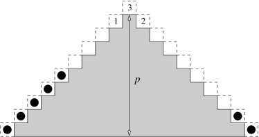
(a) Case $|T(\Pi)|=1$.

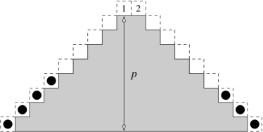
(b) Case $|T(\Pi)|\geq 2$.

Figure 5: Structure of the fixed points.

3.3 A kind of magic

From Corollary 6, we know that for any $n\in\mathbb{N}$, the configuration $(n)$ leads to at least one fixed point. In this section we compute precisely the number of fixed points of SSPM with initial condition $(n)$.

In order to understand how a fixed point can be obtained, we try to give a visual construction. Consider Figures 5. The $n$ grains of the fixed point must be arranged in the grayed part and can partially occupy the dashed frame with the supplementary constraint that grains in the dashed part must be as much clustered to the ground as possible. Boxes labeled $1$, $2$ and $3$ in Figures 5(a) and 5(b) cannot be filled (for more details see the proof of Lemma 14). Remark that if $p$ is the height of the grayed part, then this area contains $p^{2}$ grains in Figure 5(a), and $p^{2}+p$ grains in Figure 5(b). Appendix A shows all the possible fixed points reachable from the initial condition $(n)$ for $n\in[1,32]$.

Lemma 14 will be the main tool that we use to count the number of fixed points, it proves that the “shapes” outlined in Figure 5(b) describe exactly all the possible fixed points. Let $g_{1}(n)$ be the numbers of fixed points $\Pi$ such that $|T(\Pi)|=1$, and $g_{2}(n)$ the numbers of fixed points $\Pi$ such that $|T(\Pi)|\geq 2$.

Lemma 14.

For any $n\in\mathbb{N}$, consider SSPM with initial condition $(n)$. The number of fixed points of $\mathcal{G}_{(n)}$ is given by $G(n)=g_{1}(n)+g_{2}(n)$.

Proof.

Let $n\in\mathbb{N}$, and $\Pi$ be a fixed point of $(n)$. If $|T(\Pi)|=1$, clearly $\Pi$ can be constructed as shown in Figure 5(a) (at most one plateau on the left and one on the right). Moreover, it cannot be constructed from Figure 5(b) since the boxes at the top (labelled $1$ and $2$) are left empty.

If $|T(\Pi)|\geq 2$, the fixed point is not represented on Figure 5(a), since the boxes labelled $1$ and $2$ cannot be filled. To show that it is constructible from Figure 5(b), let $L(\Pi)=[1,t]$ and $R(\Pi)=[t+1,k]$ be a crazed decomposition of $\Pi=(\Pi_{1},\ldots,\Pi_{k})$. If $\Pi_{t}=\Pi_{t+1}$, cut Figure 5(b) in two parts at the middle of the configuration. It is clear that $L(\Pi)$ fits in the left part (at most one plateau), and $R(\Pi)$ fits in the right part for the same reason. If $\Pi_{t}=\Pi_{t+1}+1$, $T(\Pi)\subset L(\Pi)$. Cut Figure 5(b) in two parts, at the right of the two grains on top of the grayed pile, $L(\Pi)$ and $R(\Pi)$ fit. The symmetrical case is similar.

Conversely, all the configurations with $n$ grains constructible from Figures 5 are clearly fixed points, are LR-decomposable, and hence are fixed points of $(n)$ (Proposition 13). Therefore, the total number of fixed points is the number of configurations constructible from Figure 5(a) plus the number of configurations constructible from Figure 5(b), i.e. $G(n)=g_{1}(n)+g_{2}(n)$. ∎

The two following lemmas give the exact expression of $g_{1}(n)$ and $g_{2}(n)$.

Lemma 15.

For any $n\in\mathbb{N}$, consider SSPM with initial condition $(n)$. The number of fixed points of $\mathcal{G}_{(n)}$ with top of length $1$ is given by

$$g_{1}(n)=\begin{cases}n-p^{2}+1&\text{if}\;n-p^{2}\leq p-1\enspace,\\ 2p-n+p^{2}-1&\text{if}\;p\leq n-p^{2}\leq 2p-1\enspace,\\ 0&\text{otherwise,}\end{cases}$$

where $p$ is the unique integer such that $p^{2}\leq n<(p+1)^{2}$.

Proof.

For $n\in\mathbb{N}$, consider a fixed point $\Pi\in\mathcal{G}_{(n)}$. Since by hypothesis $|T(\Pi)=1|$, the overall structure is illustrated in Figure 5(a). As $n$ is fixed, we can determine $p$: it is the unique integer satisfying $p^{2}\leq n<(p+1)^{2}$, i.e. $p=\lfloor\sqrt{n}\rfloor$. Now, let $u=n-p^{2}$ be the number of grains left after having arranged the grayed zone. Distributing these $u$ grains consecutively and in all possible manners on the borders of the grayed zone starting from bottom to top gives all possible fixed points (lemma 14). To be more precise we must distinguish three cases:

• $0\leq u<p$: we put all $u$ grains in the free boxes on the left, from bottom to top; this gives a fixed point. Then we put only $u-1$ grains on the left and $1$ in the free box at the bottom on the right; this gives another fixed point. This process is iterated until there are $0$ gains on the left and $u$ on the right. It is clear that this procedure gives $u+1$ fixed points.

• $p\leq u\leq 2p-2$: we start by putting $p-1$ grains in the free boxes on the left, and the remaining $u-p+1$ grains in the free boxes on the right, starting from bottom to top; this gives a fixed point. Then we put only $p-2$ grains on the left and the $u-p+2$ remaining grains in the free boxes on the right, proceeding from bottom to top; this gives another fixed point. Then, we can put $p-3$ grains on the left and so on until there are $p-1$ grains on the right. It is clear that $(p-1)-(u-p+1)+1=2p-u-1$ distinct fixed points can be generated in this manner.

• $u=2p-1$ or $u=2p$; then there are necessarily $p$ grains on the left or on the right, hence there is one grain in box 1 or 2 (Figure 5(a)). This should not be allowed, as it would mean that $|T(\Pi)|>1$, which is not the case. In this last case, there are $0$ fixed points.

Finally, remark that box number $3$ is not taken into account either, since it would mean that all dashed boxes are filled and therefore we would have chosen $p+1$ as height of the pile instead of $p$. ∎

Lemma 16.

For any $n\in\mathbb{N}$, consider SSPM with initial condition $(n)$. The number of fixed points of $\mathcal{G}_{(n)}$ with top of length bigger than $1$ is given by

$$g_{2}(n)=\begin{cases}n-p^{2}-p+1&\text{if}\;n-p^{2}-p\leq p-1\enspace,\\ p&\text{if}\;n-p^{2}-p=p\enspace,\\ 3p-n+p^{2}+1&\text{if}\;p+1\leq n-p^{2}-p\leq 2p+1\enspace,\\ \end{cases}$$

where $p$ is the unique integer such that $p^{2}+p\leq n<(p+1)^{2}+(p+1)$.

Proof of 16.

The proof is similar to the one of Lemma 15. For $n\in\mathbb{N}$, consider a fixed point $c\in\mathcal{G}_{(n)}$. By hypothesis $|T(c)|\geq 2$, therefore the overall structure is the one illustrated in Figure 5(b). Since $n$ is fixed, we can determine $p$: it is the unique integer satisfying $p^{2}+p\leq n<(p+1)^{2}+(p+1)$. Let $v=n-p^{2}-p$ be the number of grains left after having arranged the grayed zone. Distributing the $v$ grains in all possible ways gives the number of fixed points $\Pi$ with $|T(\Pi)|\geq 2$ (Lemma 14). Again, we must distinguish three cases:

• $0\leq v<p$: we put all $v$ grains in the free boxes on the left from bottom to top; this gives a fixed point. Then we put only $v-1$ grains on the left and $1$ in the free box on the right at the bottom; this gives another fixed point. This can be iterated until there are 0 grains on the left and $v$ on the right. It is clear that this procedure gives $v+1$ fixed points.

• $v=p$: again, we can put $p$ grains on the left, $0$ on the right and so on until there are $0$ on the left, $p$ on the right. Therefore there should be $p+1$ fixed points, but in fact the first one and the last one are exactly the same: top of length 3, and no plateaus. What happens is that the reference column is not at the same position, it is shifted by one, which does not matter. This is the only case of duplicated fixed point.

• $p<v\leq 2p+1$: we start by putting $p$ grains in the free boxes on the left, and the remaining $v-p$ grains in the free boxes on the right, starting from bottom to top; this gives a fixed point. Then we put only $p-1$ grains on the left and the $v-p+1$ remaining grains on the free boxes to the right, proceeding from bottom to top; this gives another fixed point. We proceed until there are $p$ grains on the right, it is clear that $p-(v-p)+1=2p-v+1$ distinct fixed points can be generated in this manner.

Remark that boxes at the top of the dashed pile must not be taken into account in the computation of the number of fixed points for it would mean that all dashed boxes are filled and therefore we would have chosen $p+1$ as height of the pile and not $p$. Moreover, if only one of them is filled, we generate a fixed point already counted in Lemma 15 (top of length $1$). ∎

The following proposition gives a closed formula for the number of fixed points in the orbit of initial condition $(n)$. The formula is somewhat “magical” since it is very simple but we have neither practical nor visual explanation for it.

Proposition 17.

For any $n\in\mathbb{N}$, consider SSPM with initial condition $(n)$. The number of fixed points of $\mathcal{G}_{(n)}$ is given by $G(n)=\lfloor\sqrt{n}\rfloor$.

Proof.

Let $n\in\mathbb{N}$ and $p=\lfloor\sqrt{n}\rfloor$ the only integer such that $p^{2}\leq n<(p+1)^{2}$, there are three cases which correspond to the cases of Lemmas 15 and 16.

• If $p^{2}\leq n\leq p^{2}+p-1$; then $(p-1)^{2}+(p-1)\leq n<p^{2}+p$. This is case $1$ for Lemma 15 and case $3$ for Lemma 16, hence from Lemma 14, $G(n)=[n-p^{2}+1]+[3(p-1)-n+(p-1)^{2}+1]=p=\lfloor\sqrt{n}\rfloor$.

• If $p^{2}+p\leq n\leq p^{2}+2p-1$; we are in case $2$ of Lemma 15 and case $1$ of Lemma 16, hence from Lemma 14, $G(n)=[2p-n+p^{2}-1]+[n-p^{2}-p+1]=p=\lfloor\sqrt{n}\rfloor$.

• If $n=p^{2}+2p$, this is case $3$ for Lemma 15 and case $2$ for Lemma 16. From Lemma 14, we find $G(n)=0+p=\lfloor\sqrt{n}\rfloor$.

∎

Remark that it would also be possible to give the exact expression of each of these fixed points, but it would be complex and of no interest here. To have an idea of what they look like, please refer to Appendix A.

Finally, remark that we did not take into account the initial position of the columns. For the same fixed point, there may exist different fixed points which have the same shape, but at different indices. In this paper we do not consider this fact, we only take into account the general shape of the configurations.

4 Conclusions and future work

In this paper we have introduced SSPM: a symmetric version of the well-known SPM model. We have proved that SSPM has fixed point dynamics and exhibited the precise structure of the fixed points which are in the orbit of initial condition $(n)$. Moreover, we showed a simple closed formula for counting the number of distinct (i.e. having different shape) fixed points. Remark that this result is surprising since the combinatorial complexity of the orbit graphs becomes higher and higher when the number $n$ of grains grows. This complexity contrasts with the simplicity of the formula for the number of fixed points: $\left\lfloor\sqrt{n}\right\rfloor$. Moreover, this formula is to some extent fascinating: although it is very simple, we have neither a practical nor a visual explanation for it.

This research can be continued along three main directions:

• Corollary 6 says that, starting from any initial configuration, SSPM has fixed point dynamics. Can we give a formula or at least tight bounds for the shortest path to a fixed point? For the longest?

• Section 3.2 gives a precise characterization of orbit graphs for initial conditions made of one single column. It would be interesting to extend this characterization to more general initial conditions or at least to find an alternative characterization.

• The model we introduced is intrinsically sequential: only one grain moves at each time step. It would be interesting to introduce a model similar to SSPM but with synchronous update. This would be even more realistic than SSPM for the simulation of natural phenomena.

Appendix A Fixed points of $(n)$ for $1\leq n\leq 32$

$n=1$

$n=2$

$n=3$

$n=4$

$n=5$

$n=6$

$n=7$

$n=8$

$n=9$

$n=10$

$n=11$

$n=12$

$n=13$

$n=14$

$n=15$

$n=16$

$n=17$

$n=18$

$n=19$

$n=20$

$n=21$

$n=22$

$n=23$

$n=24$

$n=25$

$n=26$

$n=27$

$n=28$

$n=29$

$n=30$

$n=31$

$n=32$

References

- [1] P. Bak, C. Tang, and K. Wiesenfeld. Self-organized criticality. Physical Review A, 38(1):364–374, 1988.
- [2] T. Brylawski. The lattice of integer partitions. Discrete mathematics, 6:201–219, 1973.
- [3] D. Dhar, P. Ruelle, S. Sen, and D. Verma. Algebraic aspects of sandpile models. Journal of Physics A, 28:805–831, 1995.
- [4] E. Formenti and B. Masson. A note on fixed points of generalized ice piles models. International Journal on Unconventional Computing, 2005. Accepted for publication.
- [5] E. Formenti and B. Masson. On computing fixed points for generalized sand piles. International Journal on Unconventional Computing, 2(1):13–25, 2005.
- [6] E. Goles and M. A. Kiwi. Games on line graphs and sandpile automata. Theoretical Computer Science, 115:321–349, 1993.
- [7] E. Goles, M. Morvan, and H. D. Phan. Sandpiles and order structure of integer partitions. Discrete Applied Mathematics, 117(1–3):51–64, 2002.
- [8] E. Goles, M. Morvan, and H. D. Phan. The structure of linear chip firing games and related models. Theoretical Computer Science, 270:827–841, 2002.
- [9] P. B. Miltersen. Two notes on the computational complexity of one-dimensional sandpiles. Technical Report RS-99-3, BRICS, 1999.
- [10] C. Moore and M. Nilsson. The computational complexity of sandpiles. Journal of Statistical Physics, 96:205–224, 1999.
- [11] P. Ruelle and S. Sen. Toppling distributions in one-dimensional abelian sandpiles. Journal of Physics A, 25:1257–1264, 1992.