Hidden Markov Process: A New Representation, Entropy Rate and Estimation Entropy

Abstract

We consider a pair of correlated processes $\{Z_{n}\}_{n=-\infty}^{\infty}$ and $\{S_{n}\}_{n=-\infty}^{\infty}$, where the former is observable and the later is hidden. The uncertainty in the estimation of $Z_{n}$ upon its finite past history $Z_{0}^{n-1}$ is $H(Z_{n}|Z_{0}^{n-1})$, and for estimation of $S_{n}$ upon this observation is $H(S_{n}|Z_{0}^{n-1})$, which are both sequences of $n$. The limits of these sequences (and their existence) are of practical interests. The first limit, if exists, is the entropy rate. We call the second limit the estimation entropy. An example of a process jointly correlated to another one is the hidden Markov process. It is the memoryless observation of the Markov state process where state transitions are independent of past observations. We consider a new representation of hidden Markov process using iterated function system. In this representation the state transitions are deterministically related to the process. By this representation we analyze the two dynamical entropies for this process, which results in integral expressions for the limits. This analysis shows that under mild conditions the limits exist and provides a simple method for calculating the elements of the corresponding sequences.

I Introduction

A stochastic process which is a noisy observation of a Markov process through a memoryless channel is called a hidden Markov process (HMP). In many applications of stochastic signal processing such as radar and speech processing, the output of the information source can be considered as an HMP. The entropy rate of HMP as the limit of compressibility of information source thus have special interest in those applications. Moreover, in the additive noise channels the noise process can be characterized as a hidden Markov process and its entropy rate is the defining factor in the capacity of channel. Finding the entropy rate of the hidden Markov process is thereby motivated by both applications in stochastic signal processing, source coding and channel capacity computation.

The study of the entropy rate of HMP started in 1957 by Blackwell [1] who obtained an integral expression for the entropy rate. This expression is defined through a measure described by an integral equation which is hard to extract from the equation in any explicit way. Bounds on the entropy rate can be computed based on the conditional entropies on sets of finite number of random variables [2]. Recent approaches for calculating the entropy rate are Monte Carlo simulation [3] and Lyapunov exponent [3],[4]. However these approaches yield indeterministic and hard to evaluate expressions. Simple expression for the entropy rate has been recently obtained for special cases where the parameters of hidden Markov source approach zero [4],[5].

The hidden Markov process is a process defined through its stochastic relation to another process. The entropy rate of HMP thus corresponds to this relation and the dynamic of the underlying process. However this entropy rate only indicates the residual uncertainty in the symbol one step ahead of observation of the process itself. It doesn’t indicate our uncertainty about the underlying process. In this paper we define estimation entropy as a variation of entropy rate to indicate this uncertainty. In general for a pair of correlated processes which one of them is hidden and the other is observable we can define estimation entropy as the long run per symbol uncertainty in the estimation of the hidden process based on the past observation. Such an entropy measure will be an important criterion for evaluating the performance of an estimator. In this paper we jointly analyze the entropy rate and estimation entropy for a hidden Markov process. This analysis is based on a mathematical model, namely the iterated function system [6], which suits the dynamics of the information state process of the HMP. This analysis results in integral expressions for these two dynamical entropies. We also derive a numerical method for iteratively calculating entropy rate and estimation entropy for HMP.

In this paper a discrete random variable is denoted by upper case and its realization by lower case. A sequence of random variables $X_{0},X_{1},X_{2},...X_{n}$ is denoted by $X_{0}^{n}$, whereas $X^{n}$ refers to $X_{-\infty}^{n}$. The probability $Pr(X=x)$ is shown by $p(x)$ (similarly for conditional probabilities), whereas $\underline{p}(X)$ represents a row vector as the distribution of $X$, ie: the $k$-th element of the vector $\underline{p}(X)$ is $Pr(X=k)$. For a random variable $X$ defined on a set ${\cal X}$, we denote by $\nabla_{\cal X}$ the probability simplex in $\mathbb{R}^{|{\cal X}|}$. A specific elements of a vector or matrix is referred to by its index in square brackets or as a subscript. The $z$-th row of matrix $A$ is represented by $A^{(z)}$. The entropy of a random variable $X$ is denoted by $H(X)$ whereas $h:\nabla_{\cal X}\rightarrow R^{+}$ represents the entropy function over $\nabla_{\cal X}$, i.e: $h(\underline{p}(X))=H(X)$ for all possible random variables $X$ on ${\cal X}$. Our notation does not distinguish differential entropies from ordinary entropies.

In the next section we define the iterated function system and draw some results from [6], as well as a new result. In section III we define the hidden Markov process by identifying the key properties for the probability distributions on the corresponding domain sets and show that such a process can be represented by an iterated function system . In sections IV and V we derive integral expressions for entropy rate and estimation entropy followed by a method for calculating them.

II Iterated Function Systems

Consider a system with a state in the space of $\Delta$, where the state transitions depends deterministically to a correlated process taking values in a set $\mathcal{I}_{m}=\{1,2,...,m\}$ and stochastically depending on the state. The mathematical model representing such a system is an iterated function system (IFS) which is defined by $m$ functions transforming a metric space $\Delta$ to itself, and $m$ place dependent probabilities.

Definition 1

A triple $\mathcal{F}=(\Delta,F_{i},q_{i})_{i=1,2...,K}$ is an iterated function system if $F_{i}:\Delta\rightarrow\Delta$ and $q_{i}:\Delta\rightarrow\mathcal{R}^{+}$ are measurable functions and $\sum_{i}q_{i}=1$.

The IFS represents the above mentioned dynamical system where the probability of event $i\in\mathcal{I}_{m}$ under state $x\in\Delta$ is $q_{i}(x)$ and the consequence of such event is the change of state to $F_{i}(x)$.

Although the generality of IFS allows the functions of $F_{i}$ and $q_{i}$ to be measurable which is a wide range of real functions, in this paper we are only interested in a subset of those functions, the continuous functions. Such systems are referred to as continuous IFS. If the functions $F_{i}$’s are only defined on $\Delta_{i}\subset\Delta$, where $\Delta_{i}=\{x\in\Delta:q_{i}(x)>0\}$, then the IFS is called partial iterated function system (PIFS). Although the general application of IFS in this paper could be involved PIFS, we avoid such complexity by restricting the application.

Consider $\mathcal{M}^{1}(\Delta)$ as the space of probability measures on $\Delta$. For an $\mathcal{F}$ we define an operator $\Phi:\mathcal{M}^{1}(\Delta)\rightarrow\mathcal{M}^{1}(\Delta),$

$$\Phi(\mu)(B)=\sum_{i}\int 1_{B}(F_{i}(x))q_{i}(x)\mu(dx),$$ (1)

for $\mu\in M^{1}(\Delta)$ and $B\subset\Delta$. The operator $\Phi$, induced by $\mathcal{F}$, represents the evolution of probability measures under the action of $\mathcal{F}$. More specifically, if our belief on the state of system at time $n$ is the probability measure $\mu_{n}$, ($\mu_{n}\in\mathcal{M}^{1}(\Delta)$), then this belief at time $n+1$ is

$$\mu_{n+1}=\Phi\mu_{n},$$ (2)

which can be easily verified by Equation (1) and role of functions $F_{i}$ and $q_{i}$. Note that the operator $\Phi$ is deterministic and it is affine, i.e: $\Phi(\lambda\mu_{1}+(1-\lambda)\mu_{2})=\lambda\Phi\mu_{1}+(1-\lambda)\Phi\mu_{2}$. By such representation $\Phi$ is a so called Markov operator.

For a Markov operator $\Phi$ acting on the space $\mathcal{M}^{1}(\Delta)$ a measure $\mu\in\mathcal{M}^{1}(\Delta)$ is invariant if $\mu=\Phi\mu$, and it is attractive if

$$\mu=\lim_{n\rightarrow\infty}\Phi^{n}\nu,$$ (3)

for any $\nu\in\mathcal{M}^{1}(\Delta)$. A Markov operator $\Phi$ (and the corresponding IFS) is called asymptotically stable if it admits an invariant and attractive measure. The concept of limit in Equations (3) is convergence in weak topology, meaning

$$\int fd\mu=\lim_{n\rightarrow\infty}\int fd(\Phi^{n}\nu),$$ (4)

for any continuous bounded function $f$. Note that the limit doesn’t necessarily exist or it is not necessarily unique. The set of all attractive measures of $\Phi$ for $\mathcal{F}$ is denoted by $\mathcal{S}^{\mathcal{F}}$.

A Markov operator which is continuous in weak topology is a Feller operator. We can show that for a continuous IFS the operator $\Phi$ is a Feller operator. In this case any $\mu\in\mathcal{S}^{\mathcal{F}}$ is invariant.

Let $B(\Delta)$ be the space of all real valued continuous bounded functions on $\Delta$. A special property of a Feller operator $\Phi:\mathcal{M}^{1}(\Delta)\rightarrow\mathcal{M}^{1}(\Delta)$ is that there exists an operator $\mathcal{U}:B(\Delta)\rightarrow B(\Delta)$ such that:

$$\int f(x)\Phi\mu(dx)=\int\mathcal{U}f(x)\mu(dx),$$ (5)

for all $f\in B(\Delta),\mu\in\mathcal{M}^{1}(\Delta)$. The operator $\mathcal{U}$ is called the operator conjugate to $\Phi$. It can be shown [6] that for a continuous IFS the operator conjugate of $\Phi$ is $\mathcal{U}$, where

$$(\mathcal{U}f)(x)=\sum_{i\in\mathcal{I}_{k}}q_{i}(x)f(F_{i}(x)).$$ (6)

For an IFS, the concept of change of state and probability of the correlated process in each step can be extended to $n>1$ steps. For an $\mathbf{i}=(i_{1},i_{2},...i_{n})\in\mathcal{I}_{m}^{n}$, we denote

$$F_{\mathbf{i}}(x)=F_{i_{n}}(F_{i_{n-1}}(...F_{i_{1}}x)...))$$

$$q_{\mathbf{i}}(x)=q_{i1}(x)q_{i2}(F_{i1}(x))...q_{in}(F_{i_{n-1}}(F_{i_{n-2}}(...F_{i1}(x))))$$

Then the probability of the sequential event $\mathbf{i}$ under state $x\in\Delta$ is $q_{\mathbf{i}}(x)$ and as a result of such sequence, the state changes from $x$ to $F_{\mathbf{i}}(x)$ in $n$ steps. As an extension of (6), we can show

$$(\mathcal{U}^{n}f)(x)=\sum_{\mathbf{i}\in\mathcal{I}_{m}^{n}}q_{\mathbf{i}}(x)f(F_{\mathbf{i}}(x)).$$ (7)

In this paper we define for a given continuous IFS, and for a $f\in B(\Delta)$,

$$\hat{F}(x)\triangleq\lim_{n\rightarrow\infty}(\mathcal{U}^{n}f)(x).$$ (8)

Now we state our result on IFS in the following Lemma which will be used in Section IV as the major application of IFS to the purpose of this paper.

Lemma 1

For a continuous IFS $\mathcal{F}=(\Delta,F_{i},q_{i})_{i=1,2...,K}$, and any function $f\in B(\Delta)$,

$$\hat{F}(x)=\int fd\mu,$$ (9)

where $\mu=\lim_{n\rightarrow\infty}\Phi^{n}\delta_{x}$ (if the limit exists), and $\delta_{x}\in\mathcal{M}^{1}(\Delta)$ is a distribution with all probability mass at $x$.

Proof:

From (5) we have

$$\int fd(\Phi^{2}\mu)=\int\mathcal{U}fd(\Phi\mu)=\int(\mathcal{U}^{2}f)d\mu,$$

where the first equality is by substituting $\mu$ with $\Phi\mu$ in (5) and the second equality by substituting $f$ with $\mathcal{U}f$. Therefore by repetition of (5), we have

$$\int fd(\Phi^{n}\mu)=\int(\mathcal{U}^{n}f)d\mu,$$ (10)

for all $f\in B(\Delta),\mu\in\mathcal{M}^{1}(\Delta)$. This results in

$$\hat{F}(x)=\lim_{n\rightarrow\infty}\int(\mathcal{U}^{n}f)d\delta_{x}=\lim_{n\rightarrow\infty}\int fd(\Phi^{n}\delta_{x})=\int fd\mu,$$

where the first equality is from the definition of $\hat{F}$ in (8) and the last one is from (4).

∎

From the above Lemma we infer that for an asymptotically stable continuous IFS, the function $\hat{F}$ is a constant independent of $x$. Note that asymptotic stability ensures that there exists at least one $\mu$ satisfying (4) for any $\nu\in\mathcal{M}^{1}(\Delta)$, which is true for $\nu=\delta_{x}$ for any $x$. If there are more than one $\mu\in\mathcal{S}^{\mathcal{F}}$, all of them has to satisfy (4). So in this case the Equality of (9) independent of $x$ is true for any $\mu\in\mathcal{S}^{\mathcal{F}}$.

We use the result of this section in the analysis of entropy measures of hidden Markov processes by specializing $\Delta$ to be the space of information state process and $f$ to be variations of the entropy function.

III The Hidden Markov Process

A hidden Markov process is a process related to an underlying Markov process through a discrete memoryless channel, so it is defined (for finite alphabet cases) by the transition probability matrix $P$ of the Markov process and the emission matrix $T$ of the memoryless channel [7],[8]. In this paper the hidden Markov process is referred to by $\{Z_{n}\}_{n=-\infty}^{\infty}$, $Z_{n}\in{\cal Z}$ and its underlying Markov process by $\{S_{n}\}_{n=-\infty}^{\infty}$, $S_{n}\in{\cal S}$. The elements of matrices $P_{|{\cal S}|\times|{\cal S}|}$ and $T_{|{\cal S}|\times|{\cal Z}|}$ are the conditional probabilities,

$$\begin{array}[]{rl}P[s,s^{\prime}]&=p(S_{n+1}=s^{\prime}|S_{n}=s),\\ T[s,z]&=p(Z_{n}=z|S_{n}=s).\end{array}$$ (11)

A pair of matrices $P$ and $T$ define a time invariant (but not necessarily stationary) hidden Markov process on the state set ${\cal S}$ and observation set ${\cal Z}$ by the following basic properties, for any $n$.

• A1: Markovity,

  $$p(s_{n}|s^{n-1})=p_{P}(s_{n}|s_{n-1}),$$ (12)

  where $p_{P}(s_{n}|s_{n-1})=P[s_{n-1},s_{n}]$.

• A2: Sufficient Statistics of State,

  $$p(s_{n}|s_{n-1},z^{n-1})=p_{P}(s_{n}|s_{n-1}),$$ (13)

  where $p_{P}(.|.)$ is defined by $P$.

• A3: Memoryless Observation,

  $$p(z^{n}|s^{n})=\prod_{i}^{n}p_{{T}}(z_{i}|s_{i}),$$ (14)

  where $p_{T}(z|s)=T[s,z]$.

Property A3 implies:

$$p(z_{n}|s_{n},z^{n-1})=p_{T}(z_{n}|s_{n}).$$ (15)

For a hidden Markov process we define two random vectors $\pi_{n}$ and $\rho_{n}$ as functions of $Z^{n-1}$ on the domains $\nabla_{\cal S},\nabla_{\cal Z}$, respectively,

$$\pi_{n}(Z^{n-1})=\underline{p}(S_{n}|Z^{n-1}).$$ (16)

$$\rho_{n}(Z^{n-1})=\underline{p}(Z_{n}|Z^{n-1}).$$ (17)

According to our notation, the random vector $\pi_{n}$ has elements $\pi_{n}[k]$, $k=1,2,...,|{\cal S}|$,

$$\pi_{n}[k]=p(S_{n}=k|Z^{n-1}),$$

and similarly for $\rho_{n}$. We obtain the relation between random vectors $\rho_{n}$ and $\pi_{n}$

$$\begin{array}[]{rl}&\rho_{n}[m](Z^{n-1})\\ &=Pr(Z_{n}=m|Z^{n-1})\\ &=\sum_{k}Pr(Z_{n}=m|Z^{n-1},S_{n}=k)Pr(S_{n}=k|Z^{n-1})\\ &=\sum_{k}Pr(Z_{n}=m|S_{n}=k)Pr(S_{n}=k|Z^{n-1})\\ &=\sum_{k}T[k,m]\pi_{n}[k](Z^{n-1}),\end{array}$$ (18)

which shows the matrix relation

$$\rho_{n}=\pi_{n}T.$$ (19)

More generally, we refer to $\zeta(\pi)\in\nabla_{\cal Z}$ as the projection of $\pi\in\nabla_{\cal S}$ under the mapping $T:\nabla_{\cal S}\rightarrow\nabla_{\cal Z}$, i.e:

$$\zeta(\pi)=\pi T.$$ (20)

We can write

$$\underline{p}(Z_{n}|\pi_{n},Z^{n-1})=\underline{p}(Z_{n}|Z^{n-1})=\rho_{n}=\zeta(\pi_{n}),$$ (21)

where the first equality is due to $\pi_{n}$ being a function of $Z^{n-1}$. Since the right hand side of (21) is (only) a function of $\pi_{n}$ (and it is a distribution on ${\cal Z}$), the left hand side must be equal to $\underline{p}(Z_{n}|\pi_{n})$, i.e: we have shown

$$\underline{p}(Z_{n}|\pi_{n})=\underline{p}(Z_{n}|\pi_{n},Z^{n-1})=\zeta(\pi_{n}).$$ (22)

This shows that $\pi_{n}$ is a sufficient statistics for the observation process at time $n$. By a similar argument we have,

$$\underline{p}(S_{n}|\pi_{n},Z^{n-1})=\underline{p}(S_{n}|Z^{n-1})=\pi_{n}=\underline{p}(S_{n}|\pi_{n}),$$ (23)

which shows that $\pi_{n}$ is a sufficient statistics for the state process at time $n$. In other words the random vector $\pi_{n}$ encapsulates all information about state at time $n$ that can be obtained form all the past observations $Z^{n-1}$. For this reason we call $\pi_{n}$ the information-state at time $n$. A similar definition for the information state with the same property has been given for the more general model of partially observed Markov decision processes in [9].

Using Bayes’ rule and the law of total probability, an iterative formula for the information state can be obtained as a function of $z_{n}$, [9], [10],

$$\pi_{n+1}=\eta(z_{n},\pi_{n}),$$ (24)

where

$$\eta(z,\pi)\triangleq\frac{\pi D(z)P}{\pi D(z)\underline{1}},$$ (25)

where $D(z)$ is a diagonal matrix with $d_{k,k}(z)=T[k,z]$, $k=1,2,..,|{\cal S}|.$

Due to the sufficient statistic property of the information state, we can consider the information state process $\{\pi_{n}\}_{n=0}^{\infty}$ on $\nabla_{\cal S}$ as the state process of an iterated function system on $\nabla_{\cal S}$ with the hidden Markov process being its correlated process. This is because the hidden Markov process at time $k$ is stochastically related to the information state process at that time by $Pr(Z_{k}=z|\pi_{k}=x)=\zeta(x)[z]$ (from (22)). On the other hand, $Z_{k}=z$ result in the deterministic change of state from $\pi_{k}=x$ to $\pi_{k+1}=\eta(z,x)$. Consequently, for a hidden Markov process there is a continuous iterated function systems defined by, for different values $z\in{\cal Z}$,

$$\begin{array}[]{rl}F_{z}(x)&=\eta(z,x),\\ q_{z}(x)&=\zeta(x)[z],\end{array}$$ (26)

where the equality $\sum_{z}q_{z}(x)=1,x\in\nabla_{\cal S}$ is satisfied due to $\zeta(x)\in\nabla_{\cal Z}$. These functions are in fact conditional probabilities, $F_{z}(x)=\underline{p}(S_{k+1}|Z_{k}=z,\pi_{k}=x)$ and $q_{z}(x)=Pr(Z_{k}=z|\pi_{k}=x)$ for any $k$.

If the emission matrix $T$ has zero entries, then function $\eta(z,x)$ could be indefinite for some $(z,x)$. This happens for those $x\in\nabla_{\cal S}$ that the element $z$ of vector $xT$ is zero, i.e: the functions $F_{z}(x)$ is only defined for $x$ that $q_{z}(x)>0$. Hence for the general choice of matrix $T$ we have a PIFS associated to the hidden Markov process. For this and other reason that will reveals later we assume that matrix $T$ has non zero entries.

For the continuous IFS related to the hidden Markov process, we can obtain the corresponding Feller operator $\Phi$ and its conjugate operator $\mathcal{U}$. The operator $\mathcal{U}$ maps any $f\in B(\Delta)$ to $\mathcal{U}f\in B(\Delta)$ where

$$\begin{array}[]{rl}(\mathcal{U}f)(x)&=\sum_{z}q_{z}(x)f(F_{z}(x))\\ =&\sum_{z}Pr(Z_{k}=z|\pi_{k}=x)f(\underline{p}(S_{k+1}|Z_{k}=z,\pi_{k}=x)).\end{array}$$ (27)

In general given $\pi_{k}=x$, the probability of a specific $n$-sequence $\mathbf{z}=(z_{1},z_{2},...,z_{n})$ for the HMP is

$$\begin{array}[]{l}Pr(Z_{k}^{k+n-1}=\mathbf{z}|\pi_{k}=x)=\\ q_{z_{1}}(x)q_{z_{2}}(F_{z_{1}}(x))...q_{z_{n}}(F_{z_{n-1}}(F_{z_{n-2}}(...F_{1}(x)))),\end{array}$$ (28)

and this sequence changes the state to

$$\pi_{k+n}=F_{z_{n}}(F_{z_{n-1}}(...F_{z_{1}}x)...)).$$

Therefore we can write

$$\underline{p}(S_{k+n}|Z_{k}^{k+n-1}=\mathbf{z},\pi_{k}=x)=F_{z_{n}}(F_{z_{n-1}}(...F_{z_{1}}x)...)).$$ (29)

Comparing to (7), we infer for any $f\in B(\Delta)$ and $\forall k$,

$$\begin{array}[]{l}(\mathcal{U}^{n}f)(x)=\\ \sum_{\mathbf{z}}Pr(Z_{k}^{k+n-1}=\mathbf{z}|\pi_{k}=x)f(\underline{p}(S_{k+n}|Z_{k}^{k+n-1}=\mathbf{z},\pi_{k}=x),\end{array}$$ (30)

For example, for entropy function $h$,

$$h(x)\triangleq\sum_{i=1}^{|{\cal S}|}-x[i]\log(x[i]),\hskip 14.45377ptx\in\nabla_{\cal S},$$ (31)

we have for any $k$,

$$(\mathcal{U}^{n}h)(x)=H(S_{k+n}|Z_{k}^{k+n-1},\pi_{k}=x).$$

The IFS corresponding to a HMP under a wide range of the parameters of the process is shown to be asymptotically stable.

Definition 2

A stochastic Matrix $P$ is primitive if there exists an $n$ such that $(P^{n})_{i,j}>0$ for all $i,j$.

Lemma 2

For a primitive matrix $P$ and an emission matrix $T$ with strictly positive entries, the IFS defined according to (26) is asymptotically stable.

Proof:

The proof follows from [6, Theorem 8.1]. The IFS $\mathcal{F}^{P}$ defined in [6, Theorem 8.1] by

$$(F_{i}^{P}(x))_{j}\triangleq\frac{\sum_{l=1}^{d}x_{l}P_{lj}T_{li}}{\sum_{l=1}^{d}x_{l}T_{li}}=\eta(i,x)[j],$$

$$q_{i}^{P}(x)\triangleq\sum_{l=1}^{d}x_{l}T_{li}=\zeta(x)[i],$$

is the same as the IFS defined by (26). It is shown in [6, Theorem 8.1] that under the conditions of this lemma $\mathcal{F}^{P}$ is asymptotically hyperbolic, which then has to be asymptotically stable according to [6, Theorem 3.4]. ∎

A Markov chain with primitive transition matrix $P$ is geometrically ergodic and has a unique stationary distribution [7].

IV Entropy Rate and Estimation Entropy

The entropy of a random variable $Z\in{\cal Z}$ is a function of its distribution $\underline{p}(Z)\in\nabla_{Z}$,

$$\begin{array}[]{rl}H(Z)=h(\underline{p}(Z))=\sum_{z}-p(z)\log p(z).\end{array}$$

For a general process $\{Z_{n}\}_{n=-\infty}^{\infty}$, the entropy of any $n$-sequence $Z_{k}^{k+n-1}$ is denoted by $H(Z_{k}^{k+n-1})$ which is defined by the joint probabilities $Pr(Z_{k}^{k+n-1}=\mathbf{z})$, for all $\mathbf{z}\in{\cal Z}^{n}$. For a stationary process these joint probabilities are invariant with $k$. The entropy rate of the process is denoted by $\hat{H}_{Z}$ and defined as

$$\hat{H}_{Z}\triangleq\lim_{n\rightarrow\infty}\frac{1}{n}H(Z_{0}^{n}),$$ (32)

when the limit exists. Let

$$\sigma_{n}\triangleq H(Z_{n}|Z_{0}^{n-1})=H(Z_{0}^{n})-H(Z_{0}^{n-1}).$$

We see that the entropy rate is the limit of Cesaro mean of the sequence of $\sigma_{n}$, i.e:

$$\hat{H}_{Z}=\lim\limits_{n\rightarrow\infty}\frac{1}{n}\sum_{i=1}^{n}\sigma_{i}.$$ (33)

We know that if the sequence of $\sigma_{n}$ converges, then the sequence of its Cesaro mean also converges to the same limit [2, Theorem 4.2.3]. However the opposite is not necessarily true. Therefore, the entropy rate is equal to

$$\hat{H}_{Z}=\lim_{n\rightarrow\infty}H(Z_{n}|Z_{0}^{n-1}),$$ (34)

when this limit exists, but the non-existence of this limit doesn’t mean that the entropy rate doesn’t exist. On the other hand, the sequence of $\sigma_{n}$ converges faster than the sequence in (33) to its limit. Therefore the convergence rate of (34) is faster than (32). This fact was first pointed out in [11].

One sufficient condition for the existence of the limit of $\sigma_{n}$ is the stationarity of the process. For a stationary process

$$\sigma_{n}=H(Z_{n+1}|Z_{1}^{n})\geq H(Z_{n+1}|Z_{0}^{n-1})=\sigma_{n+1}\geq 0,$$ (35)

which shows that $\sigma_{n}$ must have a limit. Therefore for a stationary process we can write entropy rate as (34). For a stationary Markov process with transition matrix $P$ the entropy rate is

$$\hat{H}_{Z}=\lim_{n\rightarrow\infty}H(Z_{n}|Z_{n-1})=H(Z_{1}|Z_{0})=\sum_{i}x[i]h(P^{(i)}),$$ (36)

where $x\in\nabla_{\cal Z}$ is the stationary distribution of the Markov process, i.e: the solution of xP=x. Of special interest to this paper is the entropy rate of the hidden Markov process.

We can extend the concept of entropy rate to a pair of correlated processes. Assume we have a jointly correlated processes $\{Z_{n}\}_{n=-\infty}^{\infty}$ and $\{S_{n}\}_{n=-\infty}^{\infty}$ where we observe the first process and based on our observation estimate the state of the other process. The uncertainty in the estimation of $S_{n}$ upon past observations $Z_{0}^{n-1}$ is $H(S_{n}|Z_{0}^{n-1})$. The limit of this sequence which inversely measures the observability of the hidden process is of practical and theoretical interests. We call this limit Estimation Entropy,

$$\hat{H}_{S/Z}\triangleq\lim_{n\rightarrow\infty}H(S_{n}|Z_{0}^{n-1}),$$ (37)

when the limit exists. Similar to entropy rate, we can consider the limit of Cesaro mean of the sequence $\beta_{n}\triangleq H(S_{n}|Z^{n-1})$ (i.e: $\lim\limits_{n\rightarrow\infty}1/n\sum_{i=1}^{n}\beta_{i}$ ) as the estimation entropy, which gives a more relaxed condition on its existence, but it will have a much slower convergence rate. However, if both limits exist, then they will be equal. If the two processes $\{Z_{n}\}_{n=-\infty}^{\infty}$ and $\{S_{n}\}_{n=-\infty}^{\infty}$ are jointly stationary, then $\beta_{n}$ is decreasing and non-negative (same as (35)), thus the limit in (37) exists. We see that for a wide range of non-stationary processes also the limits in (34) and (37) exist.

Practical application of estimation entropy is for example in sensor scheduling for observation of a Markov process [12]. The aim of such a scheduler is to find a policy for selection of sensors based on information-state which minimizes the estimation entropy, thus achieving the maximum observability for the Markov process. This entropy measure could also be related to the error probability in channel coding. The more the estimation entropy, the more uncertainty per symbol in the decoding process of the received signal, thus higher error probability. The estimation entropy can be viewed as a benchmark for indicating how well an estimator is working. It is the limit of minimum uncertainty that an estimator can achieve for estimating the current value of the unobserved process under the knowledge of enough history of observations. We consider HMP as a joint process and analyze its estimation entropy.

For a stationary hidden Markov process the entropy rate $\hat{H}_{Z}$ and estimation entropy $\hat{H}_{S/Z}$ are the limiting expectations

$$\begin{array}[]{rl}\hat{H}_{Z}&=\lim\limits_{n\rightarrow\infty}E[h(\rho_{n})],\\ \hat{H}_{S/Z}&=\lim\limits_{n\rightarrow\infty}E[h(\pi_{n})].\end{array}$$ (38)

However since $\pi_{n}$ and $\rho_{n}$ are functions of joint distributions of random variables $Z_{0}^{n-1}$ these expectations are not directly computable. We use the IFS for a hidden Markov process to gain insight into these entropy measures in a more general setting without the stationarity assumption.

Adapting Equation (1) with special functions $F_{z}(x)$ and $q_{z}(x)$ in 26, we obtain the Feller operator $\Phi$ for the IFS corresponding to a hidden Markov process.

$$\Phi(\mu)(B)=\sum_{z}\int\limits_{\nabla_{\cal S}}1_{B}(\eta(z,x))\zeta(x)[z]\mu(dx).$$ (39)

To analyze the entropy measures $\hat{H}_{Z}$ and $\hat{H}_{S/Z}$, we define two intermediate functions

$$\begin{array}[]{rl}\hat{H}_{Z}(x)&=\lim\limits_{n\rightarrow\infty}H(Z_{n}|Z_{0}^{n-1},\pi_{0}=x),\\ \hat{H}_{S/Z}(x)&=\lim\limits_{n\rightarrow\infty}H(S_{n}|Z_{0}^{n-1},\pi_{0}=x).\end{array}$$ (40)

In comparison to (34) and (37), these functions are the corresponding per symbol entropies when it is conditioned on a specific prior distribution of state at time $n=0$. We now use Lemma 1 to obtain an integral expressions for these limiting entropies.

Lemma 3

For a hidden Markov process

$$\begin{array}[]{rl}\hat{H}_{Z}(x)&=\int\limits_{\nabla_{\cal S}}(h_{1}\circ\zeta)d\mu,\\ \hat{H}_{S/Z}(x)&=\int\limits_{\nabla_{\cal S}}h_{2}d\mu,\\ \end{array}$$ (41)

where $\mu=\lim_{n\rightarrow\infty}\Phi^{n}\delta_{x}$, and $h_{1}:\nabla_{\cal Z}\rightarrow\mathbb{R}^{+}$ and $h_{2}:\nabla_{\cal S}\rightarrow\mathbb{R}^{+}$ are entropy functions.

Proof:

From definition of conditional entropy we write,

$$\begin{array}[]{l}H(Z_{n}|Z_{0}^{n-1},\pi_{0}=x)=\\ \sum_{\mathbf{z}}Pr(Z_{0}^{n-1}=\mathbf{z}|\pi_{k}=x)h_{1}(\underline{p}(Z_{n}|Z_{0}^{n-1}=\mathbf{z},\pi_{0}=x)).\end{array}$$ (42)

Now since (as in (18), using $p(z_{n}|s_{n},z^{n-1},\pi_{0})=p(z_{n}|s_{n})$),

$$\underline{p}(Z_{n}|Z_{0}^{n-1}=\mathbf{z},\pi_{0}=x)=\zeta(\underline{p}(S_{n}|Z_{0}^{n-1}=\mathbf{z},\pi_{0}=x)),$$ (43)

Equation (42) can be written as

$$\begin{array}[]{l}H(Z_{n}|Z_{0}^{n-1},\pi_{0}=x)=\\ \sum_{\mathbf{z}}Pr(Z_{0}^{n-1}=\mathbf{z}|\pi_{k}=x)h_{1}\circ\zeta(\underline{p}(S_{n}|Z_{0}^{n-1}=\mathbf{z},\pi_{0}=x)).\end{array}$$ (44)

Similarly from definition of conditional entropy, we can write

$$\begin{array}[]{l}H(S_{n}|Z_{0}^{n-1},\pi_{0}=x)=\\ \sum_{\mathbf{z}}Pr(Z_{0}^{n-1}=\mathbf{z}|\pi_{k}=x)h_{2}(\underline{p}(S_{n}|Z_{0}^{n-1}=\mathbf{z},\pi_{0}=x)).\end{array}$$ (45)

Comparing Equations (44) with (30), we have

$$\hat{H}_{Z}(x)=\lim\limits_{n\rightarrow\infty}(\mathcal{U}^{n}(h_{1}\circ\zeta))(x).$$ (46)

Similarly by (45),

$$\hat{H}_{S/Z}(x)=\lim\limits_{n\rightarrow\infty}(\mathcal{U}^{n}h_{2})(x).$$ (47)

Now considering Equation (8) and applying Lemma 1 we obtain (41). ∎

Lemmas 2 and 3 result in integral expressions for entropy rate and estimation entropy.

Theorem 1

For a hidden Markov process with primitive matrix $P$ and the emission matrix $T$ with strictly positive entries,

$$\begin{array}[]{rl}\hat{H}_{Z}&=\int\limits_{\nabla_{\cal S}}(h_{1}\circ\zeta)d\mu,\\ \hat{H}_{S/Z}&=\int\limits_{\nabla_{\cal S}}h_{2}d\mu,\\ \end{array}$$ (48)

where $\mu$ is any attractive and invariant measure of operator $\Phi$, and $h_{1},h_{2}$ are the entropy functions on $\nabla_{\cal Z},\nabla_{\cal S}$, respectively.

Proof:

From Lemma 2, under the condition of this Theorem, the continuous IFS corresponding to the HMP is asymptotically stable. As it is discussed after Lemma1, in this case the functions $\hat{H}_{Z}(x)$ and $\hat{H}_{S/Z}(x)$ (in (46) and (47)) are independent of $x$ and the equalities of (41) are satisfied for any attractive measure (which exists and it is also an invariant measure) of $\Phi$. The independency of $x$ for $\hat{H}_{Z}(x)$ and $\hat{H}_{S/Z}(x)$ in (40) results in the equalities in (48) for $\hat{H}_{Z}$ and $\hat{H}_{S/Z}$. Note that for a set of random variables $X,Y,Z$ if $H(Y|Z,X=x)$ is invariant with $x$, then $H(Y|Z)=H(Y|Z,X)=H(Y|Z,X=x)$. Moreover from the existence of limit of $\sigma_{n}$ (defined before) this limit is equal to $\hat{H}_{Z}$. ∎

The first equality in the above theorem has been previously obtained by a different approach in [13]. However in [13], the measure $\mu$ is restricted to be $\mu=\lim\limits_{n\rightarrow\infty}\Phi^{n}\delta_{x^{*}}$, where $x^{*}$ is the stationary distribution of the underlying Markov process defined by $P$,

$$x^{*}P=x^{*}.$$ (49)

The integral expression for $\hat{H}_{Z}$ in Theorem 1 is also the same as the expression in [6, Proposition 8.1] for $\theta=P$. For this case the integral expression is shown to be equal to both of the following two entropy measures

$$\begin{array}[]{rl}\mathcal{H}(x^{*})&\triangleq\lim\limits_{n\rightarrow\infty}\frac{1}{n}\sum_{\mathbf{z}\in{\cal Z}^{n}}q_{\mathbf{z}}(x^{*})\log(q_{\mathbf{z}}(x^{*})),\\ \mathcal{H}(\mu)&\triangleq\lim\limits_{n\rightarrow\infty}\frac{1}{n}\sum_{\mathbf{z}\in{\cal Z}^{n}}\int q_{\mathbf{z}}(x)\mu(dx).\log(\int q_{\mathbf{z}}(x)\mu(dx)),\end{array}$$ (50)

where $\mu$ is the attractive and invariant measure of $\Phi$ for the IFS defined by (26). Considering $q_{\mathbf{z}}(x)=p(Z_{0}^{n-1}=\mathbf{z}|\pi_{0}=x)$ for HMP, (c.f. (28)), the two equalities match with Lemma 3 and Theorem 1. However, the analysis in [6] is based on a general and complex view to dynamical systems, where the dynamics of system is represented by a Markov operator and the measurement process is separately represented by a Markov pair, and this Markov pair corresponds to a PIFS.

The integral expression for $\hat{H}_{Z}$ is also equivalent to the original Blackwell’s formulation [1] by a change of variable $x$ to $xP$. This is because the expression in [1] is derived based on $\alpha_{n-1}=\underline{p}(S_{n-1}|Z^{n-1})$ instead of $\pi_{n}=\alpha_{n-1}P$ in (16) (cf. (13)). The measure of integral also corresponds to this change of variable. Note that the measure $\mu$ in (48) satisfies (due to its invariant property)

$$\mu(B)=\Phi(\mu)(B)=\sum_{z}\int_{F_{z}^{-1}(B)}(xT)[z]\mu(dx),$$ (51)

(cf. (39)) which is the same as the integral equation for the measure in [1] if we change the integrand of (51) to $r_{z}(x)=(xPT)[z]$ and instead of $F_{z}(x)$ use the function $f_{z}(x)=xPD(z)/r_{z}(x)$ (derived from (25) by $\pi=\alpha P$, satisfying $\alpha_{n+1}=f_{z}(\alpha_{n})$).

V A Numerical Algorithm

Here we obtain a numerical method for computing entropy rate and estimation entropy based on Lemma 3 and the fact that with the condition of Theorem 1, (41) is independent of $x$. The computational complexity of this method grows exponentially with the iterations, but numerical examples show a very fast convergence. In [14] it is shown that applying this method for computation of entropy rate yields the same capacity results for symmetric Markov channels similar to previous results.

We write (41) as

$$\begin{array}[]{rl}\hat{H}_{Z}(\nu)&=\lim\limits_{n\rightarrow\infty}\int\limits_{\nabla_{\cal S}}(h_{1}\circ\zeta)d\mu_{n},\\ \hat{H}_{S/Z}(\nu)&=\lim\limits_{n\rightarrow\infty}\int\limits_{\nabla_{\cal S}}h_{2}d\mu_{n},\\ \end{array}$$ (52)

where $\mu_{n}=\Phi^{n}\delta_{\nu}$. Considering $\overline{\mu}_{n}:\nabla_{\cal S}\rightarrow\mathcal{R}$ as the probability density function corresponding to the probability measure $\mu_{n}$, from (2) and (39) we have the following recursive formula

$$\overline{\mu}_{n+1}(\pi_{n+1})=\sum_{z}\int\limits_{\nabla_{\cal S}}\delta(\pi_{n+1}-\eta(z,\pi_{n}))\zeta(\pi_{n})[z]\overline{\mu}_{n}(\pi_{n})d\pi_{n}.$$ (53)

Corresponding to the initial probability measure $\delta_{\nu}$, we have the initial density function $\overline{\mu}_{0}(x)=\delta(x-\nu)$. By $\overline{\mu}_{0}$ being a probability mass function, Equation (53) yields a probability mass function $\overline{\mu}_{n}$ for any $n$. For example $\overline{\mu}_{1}(.)$ is

$$\overline{\mu}_{1}(\pi_{1})=\sum_{z}\delta(\pi_{1}-\eta(z,\nu))\zeta(\nu)[z],$$

which is a $|{\cal Z}|$ point probability mass function. By induction it can be shown that the distribution $\overline{\mu}_{n}(.)$ for any $n$ is a probability mass function over a finite set $U_{n}$ which consists of $|{\cal Z}|^{n}$ points of $\nabla_{{\cal S}}$, $U_{n}=\{u\in\nabla_{{\cal S}}:u=\eta(z,v),z\in{\cal Z},v\in U_{n-1}\}$, $|U_{n}|=|{\cal Z}|^{n}$, $U_{0}=\{\nu\}$. The probability distribution over $U_{n}$ is $\dot{\mu}_{n}(u)=\dot{\mu}_{n-1}(v)\zeta(v)[z]$ for $u=\eta(z,v)$, $v\in U_{n-1}$. Therefore for every $v\in U_{n-1}$, $|{\cal Z}|$ points will be generated in $U_{n}$ that corresponds to $\eta(z,v)$ for different $z$, and the probability of each of those points will be $\dot{\mu}_{n-1}(v)(vT)[z]$.

Starting from $U_{0}=\{\nu\}$ for some $\nu\in\nabla_{\cal S}$, by the above method we can iteratively generate the sets $U_{n}$ and the probability distribution $\dot{\mu}_{n}(.)$ over these sets. The integrals in (52) can now be written as summation over $U_{n}$, therefore the entropy rate and estimation entropy are the limit of the following sequences

$$\begin{array}[]{rl}H_{Z}^{n}&=\sum_{i=1}^{|{\cal Z}|^{n}}\dot{\mu}_{n}(u_{i})h_{1}(u_{i}T),\hskip 14.45377ptu_{i}\in U_{n},\\ H_{S/Z}^{n}&=\sum_{i=1}^{|{\cal Z}|^{n}}\dot{\mu}_{n}(u_{i})h_{2}(u_{i}),\hskip 14.45377ptu_{i}\in U_{n},\end{array}$$ (54)

where

$$\begin{array}[]{rl}h_{1}(\rho)&=-\sum_{z}\rho[z]\log\rho[z]$, $\rho\in\nabla_{\cal Z},\\ h_{2}(\pi)&=-\sum_{s}\pi[s]\log\pi[s]$, $\pi\in\nabla_{\cal S}.\end{array}$$

Figure 1 shows the convergence of the proposed method to the entropy rate and estimation entropy for various starting points $\nu$ for an example hidden Markov process. In this example ${\cal S}={\cal Z}=\{0,1,2,3\}$, and

$$P=\left(\begin{array}[]{cccc}.02&.03&.05&.9\\ .8&.06&.04&.1\\ .1&.7&.15&.05\\ .9&.03&.03&.04\end{array}\right),T=\left(\begin{array}[]{cccc}.1&.2&.5&.2\\ .6&.1&.2&.1\\ .5&.2&.1&.2\\ .3&.2&.1&.4\end{array}\right).$$

Although the result of Section IV ensures convergence of algorithm for any starting distribution $\nu$, this figure and other numerical examples show faster convergence for $\nu=x^{*}$ (the solution of (49)). Without the condition of Theorem 1, the convergence could be to different values for various $\nu$. Among various examples of HMP, the convergence will be slower where the entropy rate of the underlying Markov process with transition probability matrix $P$ ($\hat{H}_{Z}$ in (36)) is very low relative to $\log_{2}|{\cal S}|$ (in the above example it is 0.678b relative to 2b) or the rows of $T$ have high entropy.

The sequence of $H^{n}_{Z}$, as the right hand side of (52) for finite $n>0$, is in fact $H_{Z}^{n}=H(Z_{n}|Z_{0}^{n-1},\pi_{0}=\nu)$. If we assume (as in [2]) that the process $Z_{n}$ starts at time zero, i.e: one sided stationary process, then $\pi_{0}$ means the distribution of state without any observation which if we further assume that it is the stationary distribution of state process, i.e: $x^{*}$ in (49), then both of the processes $\{Z_{n}\}_{n=-\infty}^{\infty}$ and $\{S_{n}\}_{n=-\infty}^{\infty}$ are stationary. So for $\nu=x^{*}$, $H_{Z}^{n}=H(Z_{n}|Z_{0}^{n-1})=\sigma_{n}$, and similarly $H_{S/Z}^{n}=H(S_{n}|Z_{0}^{n-1})=\beta_{n}$, and the sequences of $\sigma_{n}$ and $\beta_{n}$ converge monotonically from above to their limits. Therefore, $H_{Z}^{n}$ and $H_{S/Z}^{n}$ as defined in (54) for $\nu=x^{*}$ are always monotonically decreasing sequence of $n$. Figure 1 exemplifies this fact.

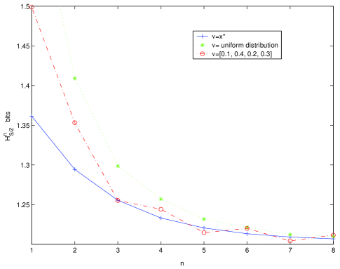
Figure 1: The convergence of the proposed algorithm to the entropy rate (left) and estimation entropy of the example hidden Markov process for various $\nu$.

VI Conclusion

HMP is a process described by its relation to a Markov state process which has stochastic transition to the next state independent of the current realization of the process. In this paper we showed that HMP can be better described and more rigorously analyzed by iterated function systems whose state transitions are deterministically related to the process. In both descriptions the state is hidden and the process at any time is stochastically related to the state at that time.

In this paper we also introduced the concept of estimation entropy for a pair of joint processes which has practical applications. The entropy rate for a process, like HMP, which is correlated to another process can be viewed as the self estimation entropy. Both entropy rate and estimation entropy for the hidden Markov process can be analyzed using the iterated function system description of the process. This analysis results in integral expressions for these dynamical entropies. The integral expressions are based on an attractive and invariant measure of the Markov operator induced by the iterated function system. These integrals can be evaluated numerically as the limit of special numerical sequences.

VII Acknowledgment

The author would like to thank Wojciech Slomczynski for bringing to attention the underpinning theories of this paper from his eminent monograph [6]. The special application of estimation entropy to scheduling problem [12] is a joint work with Bill Moran and Sofia Suvorova.

References

- [1] D.Blackwell, ”The entropy of functions of finite-state Markov chains”, Trans. First Prague Conf. Inf. Th., Statistical Decision Functions, Random Processes, page 13-20, 1957.
- [2] T.M.Cover and J.A.Thomas. ”Elements of Information Theory”, Wiley, New York, 1991.
- [3] T. Holiday, P. Glynn, and A. Goldsmith,” Capacity of finite state Markov channels with general inputs”, Int. Symp. Inf. Th., Japan, July 2003.
- [4] P.Jacquet, G.Seroussi, and W. Szpankowski,”On the entropy rate of a hidden Markov process. Int. Symp. Inf. Th., p.10, Chicago, IL, July 2004.
- [5] E. Ordentlich and T. Weissman” New Bounds on the Entropy Rate of Hidden Markov Processes”, San Antonio IT Workshop, October 2004.
- [6] W. Slomczynski. ”Dynamical Entropy, Markov Operators and Iterated Function Systems”, Wydawnictwo Uniwersytetu Jagiellonskiego, ISBN 83-233-1769-0, Krakow, 2003.
- [7] Y. Ephraim and N. Merhav, ”Hidden Markov Processes,” IEEE Trans. Inform. Theory, vol. IT-48 No.6 , pp. 1518-1569, June 2002.
- [8] L.R. Rabiner, ”A tutorial on hidden Markov models and selected applications in speech recognition”, Proceedings of the IEEE, vol 77, No 2, February 1989, pp. 257-286.
- [9] R.D. Smallwood and E.J. Sondik, ”Optimal control of partially observed Markov processes over a finite horizon,” Operation Research, vol.21, pp. 1071-1088, 1973.
- [10] A. Goldsmith and P Varaiya, “ Capacity, Mutual Information, and Coding for Finite-State Markov Channels,” IEEE Trans. Inform. Theory, vol. IT-42 No.3 , pp. 868–886, May 1996.
- [11] C. E. Shannon, “A mathematical theory of communication,” Bell Syst. Tech. J., vol, 27, pp. 379–423 and 623–656, 1948.
- [12] —, ”Minimum entropy scheduling for hidden Markov procesess,” Raytheon Systems Company internal report, Integrated Sensing Processor Phase II. March 2006.
- [13] M. Rezaeian, “The entropy rate of the hidden Markov process,” submitted to IEEE Trans. Inform. Theory, May 2005.
- [14] M. Rezaeian, “Symmetric characterization of finite state Markov channels,” IEEE Int. Symp. Inform. Theory, July 2006, Seattle, USA.