Uniform Random Sampling of Traces in Very Large Models

Abstract

This paper presents some first results on how to perform uniform random walks (where every trace has the same probability to occur) in very large models. The models considered here are described in a succinct way as a set of communicating reactive modules. The method relies upon techniques for counting and drawing uniformly at random words in regular languages. Each module is considered as an automaton defining such a language. It is shown how it is possible to combine local uniform drawings of traces, and to obtain some global uniform random sampling, without construction of the global model.

1 Introduction

Model based testing has received a lot of attention for years and is now a well established discipline (see for instance [27, 8]). Most approaches have focused on the deterministic derivation from a finite model of some so-called checking sequence, or of some complete/exhaustive set of test sequences, that ensure conformance of the implementation under test ($IUT$) with respect to the model. However, in very large models, such approaches are not practicable and some selection strategy must be applied to obtain tests of reasonable size. A popular selection criterion is transition coverage. Other selection methods rely upon the statement of some test purpose.

With the emergence of model checking, several sophisticated techniques for the representation and the treatment of models and formulas have been proposed and used for developing powerful verification tools for large models. Among them, one can cite: symbolic model checking, partial-order reduction methods, reactive modules, symmetry reduction, hash compaction and bounded model checking.

In this area, several authors have recently suggested the use of random walks in the state space of very large models in order to get good approximate checks in cases where exhaustive check is too expensive [31, 18, 16, 30]. This is in the line of testing methods developed earlier in the area of communication protocols [33, 28, 26, 9].

A random walk [1] in the state space of a model is a sequence of states $s_{0}$, $s_{1}$, $\ldots$ , $s_{n}$ such that $s_{i}$ is a state that is chosen uniformly at random among the successors of the state $s_{i-1}$, for i = 1, $\ldots$, n. It is easy to implement and only requires local knowledge of the model. In [33] West reported experiments where random walk methods had good and stable error detection power. In [28], Mihail and Papadimitriou identified some class of models that can be efficiently tested by random walk exploration: the random walk converges to the uniform distribution over the state space in polynomial time with respect to the size of the model. These were first evidence of the interest of such approaches for dealing with special classes of large models.

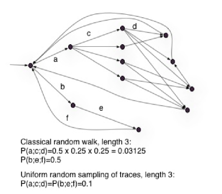
Figure 1: The case of irregular topology

However, as noted by Sivaraj and Gopalakrishnan in [31], random walk methods have some drawbacks. In case of irregular topology of the underlying transition graph, uniform choice of the next state is far from being optimal from a coverage point of view (see Figure 1). Moreover, for the same reason, it is generally not possible to get any estimation of the test coverage obtained after one or several random walks: it would require some complex global analysis of the topology of the model. One way to overcome these problems has been proposed by Gouraud et al. for program testing in [15, 11]. It relies upon techniques for counting and drawing uniformly at random combinatorial structures. Two major approaches have been developed for dealing with these problems: The Markov Chain Monte-Carlo approach (see e.g. the survey by Jerrum and Sinclair [22]) and the so-called recursive method, as described by Flajolet et al. in [14] and implemented in [32]. Although the former is more general in its applications, we chose to work with the latter because it is particularly efficient for generating the kind of random walks we deal with. The idea in [15, 11] is to give up the uniform choice of the next state and to bias this choice according to the number of elements (traces, or states, or transitions) reachable via each successor. Considering the number of traces makes it possible to ensure a uniform probability on traces. Considering elements, such as states or transitions, makes it possible to maximise the minimum probability to reach such an element.

For addressing very large models, it seems interesting to study how to combine this improved version of random walk with the representation techniques developed for struggling against combinatorial state explosions. In this paper we present some first results on how to uniformly sample traces in models described as a set of interacting transition systems, using the so-called “reactive modules” notation. This language, defined by Alur and Henzinger in [3] is used as input of the Mocha model checkers and its variants [2, 4].

In the probabilistic model checking community, it is the input language of the PRISM [29, 24] and APMC [5] model checkers. It is similar to communicating extended state machines, where transitions can be labelled by probabilities. We propose some way, inspired from [11], for uniformly random sampling traces in systems described by reactive modules, without constructing the global model. This method opens interesting perspectives for random model based testing, for model checking, and for simulation methods.

The paper is organised in two parts.

In Section 2, we first describe in 2.1 the reactive modules notation; then, in 2.2, we show how to implement classical random walk in systems described by reactive modules; in 2.3 we give an approximation of the detection power of such methods.

In Section 3 we address the computation of probabilities for improving random walk by uniformly drawing traces in models given as a set of such modules: 3.1 and 3.2 recall some results on automata and on counting and drawing uniformly at random words of a given length, in regular languages; we generalise these techniques to shuffles of such languages; 3.3 and 3.4 deal with uniform generation of traces for systems described by reactive modules, without, and then with, synchronisation.

2 Random walks in “reactive modules”

Our approach is based on a rather classical kind of model in testing, namely transition systems where transitions are labelled by atomic actions of a given language $Act$.

Definition 1

An action-labelled transition system
($ALTS$) is a structure $\mathcal{M}=(S,T,s_{0},Act)$ where $S$ is a set of states, $s_{0}$ the initial state, $T\subseteq S\times Act\times S$ a transition relation and $Act$ a set of actions.

In this paper we consider finite $ALTS$. Note that, with this definition, $ALTS$ may be non deterministic: the transition relation may associate several target states to a given state and a given action.

2.1 Reactive Modules

In this paper, we use the Reactive Modules language [3] for describing $ALTS$. This language is used in the probabilistic model checking community for modeling programs and protocols as transition systems. Two model checkers are using a subset of it as input language: PRISM [24, 29] and APMC [5].

In this language, transition systems are represented by modules that can interact together. Each module is composed of local variables and guarded commands. The global state of the system is given by the local states (i.e. the values of the local variables) of the modules. More precisely, at any moment the global state of the system is represented by a vector containing the values of all the variables of the system. A guarded command is a description of an atomic transition. It is written as

[sync] guard -> act1 + ... + actk ;

where guard is a propositional formula over the variables of the system and where each action (act1,…,actk) defines a new assignment of some local variables. The choice of the action to be activated is done non deterministically among those with a valid guard.

Basically, to compute an execution of the whole system, the algorithm is the following (when there is no synchronization):

1. Choose non deterministically one of the modules.

2. Check all the guards of the module, keep a list of the valid guards.

3. If there is no valid guards, no action can be executed, then the execution is stopped (to avoid livelock situation).

4. Choose non deterministically among the valid guards, execute non deterministically one of the corresponding actions.

5. Modify the local state, thus inducing a modification of the global state.

6. Go to step 1.

Moreover, one can see that there is a specific field in the guarded command: [sync]. This field is used to synchronize modules. By putting a synchronization between guards of different modules, we force the actions associated to the guards to be done together (this is a way to describe succinctly a complex behaviour). Basically, we have to maintain, together with the valid guards, the corresponding synchronisations. At the step 2 of the computation, a guard $g$ synchronised by $s$ in a module $m$ is considered valid if and only if the guard is true and if there exists, in each module, at least one guard which is true and synchronised by $s$. If $g$ is picked at the step 4, then in each module one of the actions corresponding to one (choosen non deterministically) of the synchronised valid guard is executed together with the one of actions of $g$.

In the following, we give an example of a simple Reactive Modules system composed of three modules. All the modules act together via synchronization. The figure 2 summarizes the example.

module timer

t : [0..1] init 0;

[tic] t=0 -> t’=1;
[tac] t=1 -> t’=0;

endmodule

module on_tic

state1 : [0..1000] init 0;

[tic] state1<1000 -> state1’=(state1+2);
[tic] state1>=1000 -> state1’=0;

endmodule

module on_tac

state2 : [1..1001] init 1;

[tac] state2<1001 -> state2’=(state2+2);
[tac] state2>=1001 -> state2’=1;

endmodule

We now explain quickly the short example. To compute executions of the model, one has to first pick one of the modules, for instance module on_tic. Then the algorithm checks the valid guards. At the beginning, the variable $state1$ is lower than 1000, so only the first guard is valid. We have to activate the first guard, but one can see that there is a synchronization on it: tic. So we have to made each module acting with the two others via a guard synchronised with tic. It means that the only valid execution is to activate the first guard of the timer and the module on_tic (there are no guards synchronised with tic in the third module). So the system starts from the initial state $(0,0,1)$. It goes from global states of the form $(0,state1,state2)$ to $(1,state1+2,state2)$, and from global states of the form $(1,state1,state2)$ to $(0,state1,state2+2)$. After a while, $state1$ (resp. $state2$) is set to $0$ (resp. $1$) and the system restart from the initial state $(0,0,1)$.

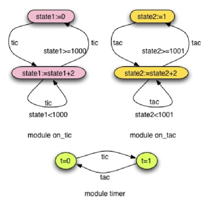
Figure 2: Scheme of the example

More informations about Reactive Modules can be found in the paper of Alur and Henzinger [3], that gives a full account of the semantics, and some correspondence between modules and transition systems.

The Reactive Modules notation, makes it possible to describe huge transitions systems via synchronised product ([6]). In practice, this notation allows to manipulate large systems without being subject to the exponential blowup of the state space (for instance systems with more than $10^{30}$ states, see [18]).

Most of the very large models come from the product of several times the same module. This is the case with classical distributed algorithms ([17]), real systems/protocols ([12, 10, 21]).

2.2 Classical random walks

An execution path, or a trace in an $ALTS$, is a finite or infinite sequence $\sigma=(s_{i},a_{i},s_{i+1})$ of transitions satisfying: for all $i\geq 0$, there exists $a_{i}\in Act$ such that $(s_{i},a_{i},s_{i+1})\in T$.

To perform a random walk in a $ALTS$ $\mathcal{M}$, it is sufficient to have a succinct representation of it, that we call $diagram_{\mathcal{M}}$, that allows to generate algorithmically, for any state $s$, the set of successors of $s$. An example of such a diagram is a set of reactive modules defining a large model $\mathcal{M}$ (as seen above). But OBDD or other representations of LTS satisfy this requirement.

The size of such a diagram can be substantially lower than the size of the corresponding $ALTS$. Typically, for Reactive Modules, the size of $diagram_{\mathcal{M}}$ is poly-logarithmic in the size of $\mathcal{M}$.

The following function Random Walk uses such a succinct representation to generate a random path of length $k$ and to check if this path leads to the detection of some conformance error. We make the simplifying assumption that there is a reliable verdict that detects an error when a fault is reached during the execution of the random walk by the implementation under test (IUT).

Random Walk
Input: $diagram_{\cal M},k$ Output: samples a path $\pi$ of length $k$ and check conformance on $\pi$ 1. Generate a random path $\pi=(s_{0},\dots,s_{k})$ such that for $i=0,\dots,k-1$, we choose uniformly $s_{i+1}$ among the successors of $s_{i}$. 2. Submit $\pi$ to the IUT. If $\pi$ detects some conformance error then return $1$ else $0$

A drawback of this approach is that we don’t know the probability distribution that it induces on the paths of the model. However, it is possible to approximate the error detection probability using approximation techniques for counting problems [23].

2.3 Randomised approximation scheme

Many enumeration and counting problems are known to be strongly intractable. For example, counting the number of elementary paths between two given nodes in the graph of a transition system is $\sharp P$-complete. We recall that $\sharp P$ is the complexity class of functions associated with counting the numbers of solutions of $NP$ decision problems. A classical method to break this complexity barrier is to approximate counting problems.

We show that we can approximate the error detection probability with a simple randomised algorithm. A probability problem is defined by giving as input a succinct representation of a transition system, a property $x$ and as output the probability measure $\mu(x)$ of the measurable set of execution paths satisfying this property. We adapt the notion of randomised approximation scheme [23] to probability problems.

Definition 2

A randomised approximation scheme for a probability problem [18] is a randomised algorithm $\mathcal{A}$ that takes an input $x$ and a real number $\varepsilon>0$ and produces a value $A(x,\varepsilon,\delta)$ such that for any $x$, $\varepsilon>0$, and $\delta>0$:

$Pr\big{(}|A(x,\varepsilon,\delta)-\mu(x)|<\varepsilon\big{)}~{}\geq~{}1-\delta$.

If the running time of $\mathcal{A}$ is polynomial in $|x|$, $\frac{1}{\varepsilon}$ and $\log(\frac{1}{\delta})$, $\mathcal{A}$ is said to be fully polynomial.

Let $Paths_{k}(s_{0})$ be the set of execution paths of origin $s_{0}$ and of depth $k$. We generate random paths in the associated probabilistic space and compute a random variable $A$ which approximates the error detection probability on the paths of depth $k$, $Prob_{k}[error]$. Consider now the random sampling algorithm $\mathcal{GAA}$ designed for the approximate computation of $Prob_{k}[error]$:

Generic approximation algorithm ${\cal GAA}$
Input: $diagram_{\cal M},k,\varepsilon,\delta$ Output: approximation of $Prob_{k}[error]$ $N:=\ln(\frac{2}{\delta})/2\varepsilon^{2}$ $A:=0$ For $i=1$ to $N$ do $A:=A+\textbf{Random Walk}(diagram_{\cal M},k)$ Return $A/N$

Our approximation will be correct with confidence $(1-\delta)$ after a number $N$ of samples polynomial in $\frac{1}{\varepsilon}$ and $\log\frac{1}{\delta}$. This result is obtained by using Chernoff-Hoeffding bounds [20] on the tail of the distribution of a sum of independent random variables.

Theorem 1

(see [25]). The generic approximation algorithm ${\cal GAA}$ is a fully polynomial randomised approximation scheme for computing $p=Prob_{k}[error]$ whenever $p\in]0,1[$.

The property of existence of conformance error detection is monotone: if it is true for a finite path $\sigma$, then it is also true for every infinite extension of this path. Let $Prob[error]$ be the error detection probability in the probabilistic space associated to the set $Paths(s_{0})$ of infinite execution paths of origin $s_{0}$. Then the sequence $(Prob_{k}[error])_{k}$ converges to the limit $Prob[error]$.

We can obtain a randomized approximation of $Prob[error]$ by increasing $k$.

Corollary 1

The fixed point algorithm defined by iterating the approximation algorithm ${\cal GAA}$ is a randomised approximation scheme for the probability problem $p=Prob[\psi]$ whenever $p\in]0,1[$.

The main interest of this randomised approximation scheme is that it allows some quantification of the error detection power of a random walk without construction and analysis of the global system.

3 Improving random walk coverage

In this section we study how to improve random walk by changing the random choice of the successors in such a way that traces are uniformly distributed. After some preliminaries, we first address the case of systems described by a set of concurrent, non synchronised reactive modules, and then we consider the case where there is some synchronisation. In both cases, we analyse the (intractable) complexity of explicitly building the product [6] of the models corresponding to the modules. Then we propose a much more efficient alternative, based on the representation of the modules, hence without explicitely constructing the whole system.

3.1 From reactive modules to automata

We briefly recall that a finite state automaton $A$ is denoted as a 5-tuple $A=\langle X,Q,q^{0},F,\Delta\rangle$ where $X$ is the alphabet, $Q$ is the finite set of states, $q^{0}$ is the initial state, $F$ is the set of final states and $\Delta:Q\times X\rightarrow Q$ is the state transition relation. A finite state automaton $A$ defines a regular language $L$ on the alphabet $X$.

Let $M_{1},M_{2},\ldots M_{r}$ be a set of reactive modules, each one standing for an ALTS. Each of the $M_{i}$’s can be represented in a straightforward way by a finite-state automaton $A_{i}=\langle X_{i},Q_{i},q^{0}_{i},F_{i},\Delta_{i}\rangle$ where

• each state of $Q_{i}$ corresponds to a state of $M_{i}$,

• any two different transitions are labelled by two different letters of $X_{i}$ (hence the cardinality of $X_{i}$ equals the numbers of transitions in $A_{i}$),

• all states are final states (hence $F_{i}=Q_{i}$).

• the $X_{i}$’s are pairwise disjoint.

Consequently, each of the $A_{i}$’s defines a regular language $L_{i}$ where each word is in one-to-one correspondence with a trace in the reactive module.

3.2 Combinatorial and algorithmic preliminaries

3.2.1 Automata and word counting

Let $L$ be a regular language and let $\ell(n)$ be the number of words of $L$ of length $n$. According to a well known result (see e.g. [13, Theorem 8.1]), there exist an integer $N_{1}$, a finite set of complex numbers $\omega_{1},\omega_{2},\ldots,\omega_{k}$ and a finite set of polynomials $R_{1}(n)$, $R_{2}(n)$, $\ldots$, $R_{k}(n)$ such that

$$n\geq N_{1}\ \rightarrow\ \ell(n)=\sum_{j=1}^{k}R_{j}(n)\omega_{j}^{n}.$$ (1)

The number $N_{1}$, as well as the $\omega_{j}$’s and the $R_{j}$’s, can be computed from an automaton of $L$, with an algorithm of polynomial complexity according to the size of the automaton. Technical details are given in Appendix 1.

If the automaton of $L$ statisfies certain conditions (see below), then there is an unique $i$ such that $|\omega_{i}|>|\omega_{j}|$ for any $j\neq i$, and $R_{i}(n)$ has degree zero, that is $R_{i}(n)=C$ for any $n$, where $C$ is a constant. Thus, if we define $\omega=\omega_{i}$, the following formula holds, asymptotically:

$$\ell(n)\sim C\omega^{n}.$$ (2)

This gives a very good estimation of $\ell(n)$ even for rather small $n$ since, according to Formulas (2) and (1), $C\omega^{n}/\ell(n)$ converges to $1$ at an exponential rate.

A simple sufficient condition for Formula (2) to hold is: the automaton is aperiodic and strongly connected. An automaton is aperiodic if, for any sufficiently large $n$, $l(n)\neq 0$. Now, as stated in Section 3.1, all the states of any automaton which represents a reactive module are final states. Thus any automaton which represents a reactive module is aperiodic. Concerning strong connectivity, it is satisfied as soon as there is a reset. Moreover, it is a sufficient yet not mandatory condition. For instance, for satisfying Formula (2), in fact it suffices to have some unique biggest strongly-connected component in the automaton. Hence, most “natural” automata are such that this formula is satisfied. Note that in the sequel we use Formula (2) for the automata corresponding to the component modules.

3.2.2 Automata and word shuffling

The shuffle of two words $w,w^{\prime}\in X^{*}$, denoted $w\,\rotatebox{-90.0}{$\exists$}\,w^{\prime}$ is the set $w\,\rotatebox{-90.0}{$\exists$}\,w^{\prime}\!=\{w_{1}w^{\prime}_{1}...w_{m}w^{\prime}_{m}|w_{i},w^{\prime}_{i}\in X^{*},w\!=\!w_{1}...w_{m},w^{\prime}\!=\!w^{\prime}_{1}...w^{\prime}_{m}\}$. For example, $ab\,\rotatebox{-90.0}{$\exists$}\,cde\,=\,\{abcde$, $acbde$, $acdbe$, $acdeb$, $cabde$, $cadbe$, $cadeb$, $cdabe$, $cdaeb$, $cdeab\}$. The shuffle operation is associative and commutative. It naturally generalises for languages: the shuffle of two languages $L_{1}$ and $L_{2}$ is the set

$$L_{1}\rotatebox{-90.0}{$\exists$}L_{2}=\bigcup_{\begin{array}[]{l}{\scriptstyle w_{1}\in L_{1},}\\ {\scriptstyle w_{2}\in L_{2}}\end{array}}w_{1}\,\rotatebox{-90.0}{$\exists$}\,w_{2}$$

This easily generalises to any finite number $r$ of languages. And the following property holds: the shuffle of a set of regular languages is a regular language. Indeed, let $r>0$ and let $L_{1},L_{2},\ldots,L_{r}$ be $r$ regular languages. Let $A_{i}=\langle X_{i},Q_{i},q_{i}^{0},F_{i},\Delta_{i}\rangle$ be an automaton of $L_{i}$, for any $1\leq i\leq r$. Then the following finite state automaton recognises $L$: $A=\langle X,Q,q_{0},F,\Delta\rangle$, where

• $X=X_{1}\cup X_{2}\cup\ldots\cup X_{r}$;

• $Q=Q_{1}\times Q_{2}\times\ldots\times Q_{r}$;

• $q_{0}=(q^{0}_{1},q^{0}_{2},\ldots,q^{0}_{r})$;

• $F=F_{1}\times F_{2}\times\ldots\times F_{r}$;

• $\Delta((q_{1},\ldots,q_{i},\ldots,q_{r}),x))=$

  $$\begin{array}[]{ll}(\Delta_{1}(q_{1},x),\ldots,q_{i},\ldots,q_{r})&\mbox{\rm if}\ x\in X_{1}\\ \ldots\\ (q_{1},\ldots,\Delta_{i}(q_{i},x),\ldots,q_{r})&\mbox{\rm if}\ x\in X_{i}\\ \ldots\\ (q_{1},\ldots,q_{i},\ldots,\Delta_{r}(q_{r},x))&\mbox{\rm if}\ x\in X_{r}\\ \end{array}$$

We call this automaton a shuffling automaton of $L_{1},L_{2},\ldots,L_{r}$.

Now let $\ell_{i}(k)$ be the number of words of length $k$ belonging to the language $L_{i}$. If the $X_{i}$’s are pairwise disjoint, then the number of words of length $n$ belonging to $L$ is:

$$\ell(n)=\!\!\!\!\!\!\sum_{k_{1}+\cdots+k_{r}=n}{n\choose k_{1},k_{2},\ldots,k_{r}}\ell_{1}(k_{1})\ell_{2}(k_{2})\ldots\ell_{r}(k_{r})$$

Now, suppose that, as in the previous section, all the $L_{i}$’s are such that

$$\ell_{i}(k)\sim C_{i}\omega_{i}^{k}$$ (3)

where $C_{i}$ and $\omega_{i}$ are two constants. Then

$$\begin{array}[]{lll}\ell(n)&\sim&C_{1}C_{2}\ldots C_{r}\!\!\!\!\!\!\!\!\displaystyle\sum_{k_{1}+\cdots+k_{r}=n}\!\!{n\choose k_{1},\ldots,k_{r}}\omega_{1}^{k_{1}}\ldots\omega_{r}^{k_{r}}\\ &=&C_{1}C_{2}\ldots C_{r}(\omega_{1}+\omega_{2}+\ldots+\omega_{r})^{n}\\ \end{array}$$ (4)

3.2.3 Uniform random generation of words in a regular language

First discussed by Hickey and Cohen[19], the method for generating words of regular languages has been improved and widely generalized by Flajolet and al [14]. The principle of the generation process is simple: Starting from state $q_{0}$, one draws a word step by step; at each step, the process consists in choosing a successor of the current state and going to it.

The problem is to proceed in such a way that only (and all) words of length $n$ can be generated, and that they are equiprobably distributed. This is done by choosing successors with suitable probabilities. Given any state $s$ of the automaton, let $g_{m}(s)$ denote the number of words of length $m$ which connect $s$ to any final state $f\in F$. Suppose that, at any step of the generation, we are on state $s$ which has $k$ successors denoted $s_{1},s_{2},\ldots,s_{k}$. In addition, suppose that $m>0$ transition remain to be done in order to get a word of length $n$. Then the condition for uniformity is that the probability of choosing state $s_{i}$ $(1\leq i\leq k)$ equals $g_{m-1}(s_{i})/g_{m}(s)$. In other words, the probability to go to any successor of $s$ must be proportional to the number of words of suitable length from this successor to any $f$.

So there is a need to compute the numbers $g_{i}(s)$ for any $0\leq i\leq n$ and any state $s$ of the automaton. This can be done by using the following recurrence relations:

$$\begin{array}[]{ccll}g_{0}(s)&=&1&\mbox{\rm if}\ s\in F\\ &=&0&\mbox{\rm otherwise}\\ g_{i}(s)&=&\sum_{s\rightarrow s^{\prime}}{g_{i-1}(s^{\prime})}&\mbox{\rm for}\ i>0\end{array}$$ (5)

where $s\rightarrow s^{\prime}$ means that there exists an letter $x\in X$ such as $(s,x,s^{\prime})\in\Delta$.

Now the generation scheme is as follows:

• Preprocessing stage: Compute a table of the $g_{i}(s)$’s for all $0\leq i\leq n$ and all states.

• Generation stage: Draw the word according to the scheme seen above.

Note that the preprocessing stage must be done only once, whatever the number of words to be generated. Easy computations show that the memory space requirement is $n\times|Q|$ integer numbers, where $|Q|$ stands for the number of states in the automaton. The number of arithmetic operations needed for the preprocessing stage, as well as for the generation stage, is linear in $n$.

3.3 Generating traces of a system of modules without synchronisation.

Here we focus on the problem of uniformly (that is equiprobably) generating traces of a given length $n$ in a system of $r$ reactive modules. In a first step, we consider that there is no synchronisation between the $r$ reactive modules $M_{i}$.

Each one is represented by a finite state automaton $A_{i}=\langle X_{i},Q_{i},q^{0}_{i},F_{i},\Delta_{i}\rangle$. As stated in Section 3.1, each of the $A_{i}$’s defines a regular language $L_{i}$ whose words correspond to the traces within the corresponding module. Since there is no synchronisation in the system, clearly there is a one-to-one correspondence between the set of traces of the system and the words of $L\,=\,L_{1}\,\rotatebox{-90.0}{$\exists$}\,L_{2}\rotatebox{-90.0}{$\exists$}\,\ldots\rotatebox{-90.0}{$\exists$}\,L_{r}$. Thus the problem reduces to uniformly generating words of length $n$ in $L$. We present two different approaches for this problem and we discuss their complexity issues.

3.3.1 Brute force method

This first approach consists in constructing the shuffling automaton that has been defined in Section 3.2.2. Then the classical algorithms for randomly generating words of a regular language can be processed, as described in Section 3.2.3.

Let $C_{1}=\sum_{0\leq i\leq r}\mbox{\rm Card}(X_{i})$ and $C_{2}=\prod_{0\leq i\leq r}\mbox{\rm Card}(Q_{i})$. The worst-case complexities of the two main steps of the algorithm are the following.

1. Constructing the automaton: This step is performed only once, whatever the number of traces to be generated. Its worst-case complexity is $C_{1}C_{2}$ in time and space requirements.

2. Generating traces: Using classical algorithms, generating one word requires $nC_{1}$ time requirement, after a preprocessing stage having worst-case complexity $nC_{1}C_{2}$ in time and space. This preprocessing stage is performed once, whatever the number of traces to be generated.

Hence the worst case complexity for generating $m$ traces of length $n$ is $O(nC_{1}C_{2}+mnC_{1})$ in time and $O(nC_{1}C_{2})$ in space. This is linear in $n$, in $m$, in the total size of the alphabets. Since $C_{2}=\prod_{0\leq i\leq r}\mbox{\rm Card}(Q_{i})$, the complexity is exponential according to the number of modules. Thus the algorithm will be efficient only for a small number of modules.

3.3.2 “On line” shuffling method

Here we describe an alternative method which avoids constructing the above automaton. We recall that $\ell_{i}(k)$ is the number of words of length $k$ belonging to the language $L_{i}$, and $\ell(k)$ is the number of words of length $k$ belonging to the language $L$. The method consists first in choosing at random, with a suitable probability, the length $n_{i}$ of each word $w_{i}$ of $L_{i}$ which will contribute to the word $w$ of $L$ to be generated. Then each $w_{i}$ is generated independently. Finally, the shuffle operation is processed. We detail the method just below.

1. Choose at random a $r$-uple $(n_{1},\ldots,n_{r})$ with probability $\Pr(n_{1},\ldots,n_{r})$ such that

   $$\Pr(n_{1},\ldots,n_{r})\ =\ \frac{{n\choose n_{1},\ldots,n_{r}}\ell_{1}(n_{1})\ldots\ell_{r}(n_{r})}{\ell(n)}$$ (6)

2. For each $0\leq i\leq r$, draw uniformly a random word $w_{i}$ of length $n_{i}$ in $L_{i}$, using the classical algorithm for generating words of a regular language.

3. Shuffle the $r$ words. This can be done with the following algorithm:

Shuffling $r$ words
Input: $r$ words $w_{1},\ldots,w_{r}$, of length $n_{1},\ldots,n_{r}$ Output: word $w$ of length $n=\sum_{i}n_{i}$ and drawn uniformly among the set of shuffles of $w_{1},\ldots,w_{r}$. $w\leftarrow\varepsilon$ $n\leftarrow\sum_{i}n_{i}$ while $n>0$ do choose an integer $i$ between $1$ and $r$ with probability $\frac{n_{i}}{n}$ add the first letter of $w_{i}$ at the end of $w$ remove the first letter of $w_{i}$ $n_{i}\leftarrow n_{i}-1$ $n\leftarrow n-1$

The word $w$ has been generated equiprobably among all the words of $L$ of length $n$. Regarding complexity issues, clearly the complexity of step 3 is linear in $n$. The complexity of step 2 is linear in $n$, in the maximum of ${\rm Card}(X_{i})$ and in the maximum of ${\rm Card}(Q_{i})$, in time as well as in space requirements. The main contribution to the total worst-case time complexity is the computation of the suitable probabilities by Formula (6). The space requirement is $O(1)$ but the number of terms in $\ell(n)$ is exponential in $n$. However, if the $L_{i}$’s satisfy the hypothesis of Formula (3), then, by Formula (4):

$$\Pr(n_{1},\ldots,n_{r})\ \sim\ \frac{{n\choose n_{1},\ldots,n_{r}}\omega_{1}^{n_{1}}\omega_{2}^{n_{2}}\ldots\omega_{r}^{n_{r}}}{(\omega_{1}+\omega_{2}+\ldots+\omega_{r})^{n}}\,.$$ (7)

There is an easy algorithm for choosing $n_{1},\ldots,n_{r}$ with this probability without computing it: take the set of integers $\{1,\ldots,r\}$ and draw a random sequence by picking independently $n$ numbers in this set in such a way that the probability to choose $i$ is $\Pr(i)=\frac{\omega_{i}}{\omega_{1}+\omega_{2}+\ldots+\omega_{r}}$. Then take $n_{i}$ as the number of occurrences of $i$ in this sequence.

Well, one could argue that Formula (7) only provides an asymptotic approximation of $\Pr(n_{1},\ldots,n_{r})$ as $n$ tends to infinity. However, as noticed in Section 3.2, the rate of convergence is exponential, so Formula (7) is precise enough even for rather small $n$. And for really small $n$ (at least when $n<N_{1}$ in Formula (1)), $\Pr(n_{1},\ldots,n_{r})$ can be computed exactly by Formulas (5) and (6).

In conclusion, for any large enough $n$, the algorithm generates traces of length $n$ almost uniformly at random. Its overall complexity is linear according to $n$, to the maximum of ${\rm Card}(X_{i})$ and to the maximum of ${\rm Card}(Q_{i})$, in time as well as in space requirements.

3.4 Generating traces in presence of synchronisation.

Now we suppose that each module contains exactly one synchronised transition, denoted $\alpha$. Thus, in the global system all modules must take $\alpha$ at the same time.

Let $A_{1},\ldots,A_{r}$ be $r$ automata, with alphabets $X_{1},\ldots,X_{r}$, all containing a common synchronisation symbol $\alpha$, such that

$$\forall i,j\in 1\ldots r,i\neq j,X_{i}\cap X_{j}=\{\alpha\}.$$

Let $S_{1},\ldots,S_{r}$ be the respective languages recognised by $A_{1},\ldots,A_{r}$. Here, any trace can be represented by a word belonging to the language $S$ defined as follows: $S$ is the set of words $w\,\in\,X_{1}\cup\ldots\cup X_{r}$ such that

$$w=w_{0}\alpha w_{1}\alpha\ldots w_{m-1}\alpha w_{m}$$

where the projection of $w$ onto any $X_{i}$ belongs to $S_{i}$. The number $m$ is the number of synchronisations during the process: each of the projections contains exactly $m$ letters $\alpha$ (and, equivalently, there is no $\alpha$ in any of the $w_{i}$.)

3.4.1 Again the brute force approach.

Here the approach consists in constructing the synchronised product of $A_{1},A_{2},\ldots,A_{r}$, as follows. Let $X_{i,\alpha}=X_{i}\setminus\{\alpha\}$. The synchronised product [6] of $A_{1},A_{2},\ldots,A_{r}$ with $\{\alpha\}$ as synchronisation set is the finite automaton $A=<X,Q,q_{0},F,\delta>$, where

• $X=X_{1}\cup X_{2}\cup\ldots\cup X_{r}$;

• $Q=Q_{1}\times Q_{2}\times\ldots\times Q_{r}$;

• $q_{0}=(q^{0}_{1},q^{0}_{2},\ldots,q^{0}_{r})$;

• $F=F_{1}\times F_{2}\times\ldots\times F_{r}$;

• $\delta$ is as follows:

  $$\begin{array}[]{l}\Delta((q_{1},\ldots,q_{i},\ldots,q_{r}),x))=\\ \hskip 28.45274pt(\Delta_{1}(q_{1},x),\ldots,q_{i},\ldots,q_{r})\ \ \mbox{\rm if}\ x\in X_{1,\alpha},\\ \hskip 28.45274pt\ldots\\ \hskip 28.45274pt(q_{1},\ldots,\Delta_{i}(q_{i},x),\ldots,q_{r})\ \ \mbox{\rm if}\ x\in X_{i,\alpha},\\ \hskip 28.45274pt\ldots\\ \hskip 28.45274pt(q_{1},\ldots,q_{i},\ldots,\Delta_{r}(q_{r},x))\ \ \mbox{\rm if}\ x\in X_{r,\alpha}.\\ \\ \Delta((q_{1},\ldots,q_{i},\ldots,q_{r}),\alpha))=\\ \hskip 28.45274pt\delta_{1}(q_{1},\alpha),\ldots,\delta_{i}(q_{i},\alpha),\ldots,\delta_{r}(q_{r},\alpha))\end{array}$$

This automaton accepts the language $S$ of synchronised traces. Once it has been built, the generation process is exactly as in Section 3.3.1, with the same time and space requirements.

3.4.2 “On line” generation of synchronised traces

Here we sketch an algorithm for almost uniformly generating random synchronised traces of length $n$, avoiding the construction of the synchronised product. The approach is similar to the one we described in Section 3.3.2, although we must be more careful because of the synchronisations. Given that each automaton $A_{i}$ contains a unique transition labeled by $\alpha$ (the synchronised transition), let $q_{i,1}$ and $q_{i,2}$ be the states just before and juste after this transition, respectively. Now let us define, for each $S_{i}$, the four following languages:

• The beginning language: $B_{i}$ is the set of words corresponding to the paths which start at the initial state of $A_{i}$, which do not cross the $\alpha$ transition, and which stop at $q_{i,1}$.

• The central language: $C_{i}$ is the set of words corresponding to the paths which start at $q_{i,2}$, which do not cross the $\alpha$ transition, and which stop at $q_{i,1}$.

• The ending language: $E_{i}$ is the set of words corresponding to the paths which start at $q_{i,2}$, which do not cross the $\alpha$ transition, and which stop anywhere.

• The non-synchronised language: $T_{i}$ is the set of words which start at the initial state of $A_{i}$, which never cross the $\alpha$ transition, and which stop anywhere.

For any $i$, the language $S_{i}$ can be defined according to $B_{i}$, $C_{i}$, $E_{i}$ and $T_{i}$:

$$S_{i}=B_{i}.(\alpha.C_{i})^{*}.\alpha.E_{i}\ \cup\ T_{i}\,.$$

Thus, if we define $B=\rotatebox{-90.0}{$\exists$}_{i=1}^{r}B_{i}$ (resp. $C=\rotatebox{-90.0}{$\exists$}_{i=1}^{r}C_{i}$, $E=\rotatebox{-90.0}{$\exists$}_{i=1}^{r}E_{i}$, and $T=\rotatebox{-90.0}{$\exists$}_{i=1}^{r}T_{i}$), we have:

$$S=B.(\alpha.C)^{*}.\alpha.E\ \cup\ T\,.$$ (8)

Now let $s(n)$ (resp. $s_{i}(n)$, $b(n)$, $b_{i}(n)$, $c(n)$, $c_{i}(n)$, $e(n)$, $e_{i}(n)$, $t(n)$, $t_{i}(n)$) be the number of words of length $n$ in $S$ (resp. $S_{i}$, $B$, $B_{i}$, $C$, $C_{i}$, $E$, $E_{i}$, $T$, $T_{i}$). Additionally, let $s(n,m)$ be the number of words of $S$ of length $n$ which contain $\alpha$ exactly $m$ times. Let $w$ be one of these words. If $m>0$, then $w$ writes $w=w_{0}.\alpha.w_{1}.\alpha.\ldots.\alpha.w_{m}$ where $w_{0}\in B$, $w_{i}\in C$ for any $1\leq i<m$, and $w_{m}\in E$. Finally, let $s(n,m,i_{0},i_{m})$ be the number of such words such that the length of $w_{0}$ equals $i_{0}$ and the length of $w_{m}$ equals $i_{m}$. Then we have

$$s(n) = \!\!\sum_{i=0}^{n}s(n,i)\,,$$ (9)

where

$$s(n,m) = \left\{\begin{array}[]{lr}t(n)&\mbox{\rm if $m=0$},\\ {\displaystyle\sum_{i_{0}+i_{m}=0}^{n-m}s(n,m,i_{0},i_{m})}&\mbox{\rm otherwise},\end{array}\right.$$ (12)

and, for $m>0$,

$$s(n,m,i_{0},i_{m})=b(i_{0})e(i_{m})\!\!\!\!\!\!\!\!\!\!\!\!\!\!\sum_{\begin{array}[]{l}{\scriptstyle i_{1}+\ldots+i_{m-1}=}\\ {\scriptstyle n-m-i_{0}-i_{m}}\end{array}}\!\!\!\!\!\!\!\!\!\!\!\!\!\!\!c(i_{1})c(i_{2})\ldots c(i_{m-1})\,.$$ (15)

Now suppose that all the the $B_{i}$’s, the $C_{i}$’s, the $E_{i}$’s and the $T_{i}$’s satisfy Formula (2), that is:

$$b_{i}(k) \sim C_{b,i}\omega_{b,i}^{k}\,,$$

$$c_{i}(k) \sim C_{c,i}\omega_{c,i}^{k}\,,$$

$$e_{i}(k) \sim C_{e,i}\omega_{e,i}^{k}\,,$$

$$t_{i}(k) \sim C_{t,i}\omega_{t,i}^{k}\,.$$

Then, similarly to Formula (4), we have:

$$b(k) \sim C_{b,1}\ldots C_{b,r}(\omega_{b,1}+\ldots+\omega_{b,r})^{k}\,,$$ (16)

$$c(k) \sim C_{c,1}\ldots C_{c,r}(\omega_{c,1}+\ldots+\omega_{c,r})^{k}\,,$$ (17)

$$e(k) \sim C_{e,1}\ldots C_{e,r}(\omega_{e,1}+\ldots+\omega_{e,r})^{k}\,,$$ (18)

$$t(k) \sim C_{t,1}\ldots C_{t,r}(\omega_{t,1}+\ldots+\omega_{t,r})^{k}\,.$$ (19)

Consequently, for $m>0$,

$$\begin{array}[]{l}s(n,m,i_{0},i_{m})\ \sim\\ \ \ \ \ \ \ (C_{b,1}\ldots C_{b,r})(C_{c,1}\ldots C_{c,r})^{m-1}(C_{e,1}\ldots C_{e,r})\\ \ \ \ \ \ \ \ \ \ \ \ \ (\omega_{b,1}+\ldots+\omega_{b,r})^{i_{0}}\\ \ \ \ \ \ \ \ \ \ \ \ \ \ \ (\omega_{c,1}+\ldots+\omega_{c,r})^{n-m-i_{0}-i_{m}}\\ \ \ \ \ \ \ \ \ \ \ \ \ \ \ \ \ (\omega_{e,1}+\ldots+\omega_{e,r})^{i_{m}}\,.\end{array}$$ (20)

Note that computing $s(n,m,i_{0},i_{m})$ requires $O(nr)$ arithmetic operations.

Now we can sketch the algorithm for generating a trace of length $n$.

1. Using Formula (20), compute $s(n,m,i_{0},i_{m})$ for all $m$ such that $1\leq m\leq n$ and for all pairs $(i_{0},i_{m})$ such that $0\leq i_{0}+i_{m}\leq n-m$. This requires $O(n^{3}\times rn)=O(rn^{4})$ arithmetic operations. Then compute $s(n,m)$ for all $m$ such that $1\leq m\leq n$, using Formula (12) and, additionally, Formula (19) when $m=0$. Finally compute $s(n)$ by Formula (9). It is worth noticing that this preliminary stage has to be done only once, whatever the number of traces of length $n$ to be generated. Its overall arithmetic complexity is $O(rn^{4})$.

2. Choose $m$, the number of synchronisations, with probability

   $$\Pr(m)={\frac{s(n,m)}{s(n)}}.$$

   Computing these probabilities requires $O(n)$ arithmetic operations in the worst case.

3. If $m=0$, then generate uniformly at random a word of length $n$ in $T$, with the same algorithm as in Section 3.3.2.

4. If $m>0$, then:

   1. Choose the length of $w_{0}$ and the length of $w_{m}$ by picking at random a pair $(i_{0},i_{m})$ with probability

      $$\Pr(i_{0},i_{m})={\frac{s(n,m,i_{0},i_{m})}{\sum_{k_{0}+k_{m}=0}^{n-m}s(n,m,k_{0},k_{m})}}\,.$$

      Computing these probabilities requires $O(n^{2})$ arithmetic operations in the worst case.

   2. Choose the lengths of $w_{1},w_{2},\ldots,w_{m-1}$ by picking at random a $(m-1)$-uple $(i_{1},i_{2},\ldots i_{m-1})$ with probability

      $$\Pr(i_{1},\ldots i_{m-1}) = {\frac{c(i_{1})c(i_{2})\ldots c(i_{m-1})}{\sum_{P}c(k_{1})c(k_{2})\ldots c(k_{m-1})}}\,.$$

      where $P$ stands for:

      $$k_{1}+k_{2}+\cdots+k_{m-1}=n-m-i_{0}-i_{m}.$$

      Using Formula (17), this reduces to

      $$\Pr(i_{1},\ldots i_{m-1}) \sim {\frac{1}{{n-2-i_{0}-i_{m}\choose m-2}}}$$ (21)

      and, similarly to Section 3.3.2, there is a simple algorithm for picking $(i_{1},i_{2},\ldots i_{m-1})$ at random with this probability. This algorithm is linear according to $n$ and $m$. The algorithm and the proof of Formula (21) are given in Appendix 2.

   3. Now we have got the whole sequence $(i_{0},i_{1},...,i_{m})$ with a suitable probability. It remains to generate the words $w_{0}\in B$, $w_{1},w_{2},\ldots,w_{m-1}\in C$ and $w_{m}\in E$, each $w_{k}$ having length $i_{k}$. Each of these words is simply a shuffle of the $r$ languages $(B_{i})_{i=1\ldots r}$ if $k=0$, $(C_{i})_{i=1\ldots r}$ if $1\leq k<m$, $(E_{i})_{i=1\ldots r}$ if $k=m$. For each of the $w_{k}$’s, the shuffling algorithm given in Section 3.3.2 can be used.

As remarked above, the first step of the algorithm, in $O(rn^{4})$ operations, has to be done only once. After that, the overall complexity of generating any random trace of length $n$ is quadratic according to $n$. And, as in Section 3.3.2, it is linear according to the maximum of ${\rm Card}(X_{i})$ and to the maximum of ${\rm Card}(Q_{i})$, in time as well as in space requirements. Thus we have defined an efficient way for approximating the uniform coverage in presence of one synchonisation for any sufficiently large $n$. The case where there are several synchronisations labelled by different symbols is more complex but we think it can be addressed with similar techniques and simplifications. This is the subject of some ongoing work.

4 conclusion and perspectives

One of the main interest of classical random walk is that it can be performed on large models with a local knowledge only. However, it presents some drawbacks, mainly related to the difficulty to estimate, without analysing the global topology, the test coverage for a given number of random walk of some given lengths. In Section 2, we have shown how it is possible to approximate it via a randomised approximation scheme.

In the rest of the paper we have described how to perform globally uniform random walks in very large models described as sets of concurrent, smaller, models. By globally uniform random walk, we mean that the choice of the successor at every step is biased in such a way that all traces of the global model have equal probability to be traversed.

A brute force approach is to count the number of paths of the desired length starting from each successor and to adjust its probability accordingly. This is feasible via techniques for counting and drawing uniformly random combinatorial structures. However, the complexity of this approach is linear in the number of states of the considered model. This makes it feasible for moderately-sized models only.

Then, we have shown how to use local uniform drawings to build globally uniform random walks, with a complexity that is linear in the size of the biggest component model. We use an estimation of the number of words, but as soon as the length of the random walks is sufficient, it is a very good approximation as seen in 3.2 (formulas (1) and (2)).

This method can be used for random testing, model checking, or simulation of protocols that involve many distributed entities, as it is often the case in practice. It ensures a balanced coverage of all behaviours, even if the topology of the underlying model is irregular.

This work is a first step only. First, we plan a campaign of experiments of the method and of some variants of it. For instance, instead of uniform coverage of traces, it is possible to consider uniform coverage of states, or of transitions as it is done in [11] for testing C programs.

Moreover, results on counting and generating combinatorial structures are not limited to words of regular languages. They open numerous perspectives in the area of random testing. A possibility that is worth to explore is the test of non deterministic systems via uniform generation of tree-like behaviours, i.e. some notion of adaptive random walk inspired from the classical notion of adaptive checking sequences [27]. It would be also interesting to study how the approach presented here for descriptions by reactive modules could be transposed to other succinct representations of large models such as OBDD, symmetry reduction, etc.

Acknowledgement. We thank Radu Grosu for interesting discussions that have motivated this work.

Appendix 1: Counting words of rational languages

Let $L$ be a language on an alphabet $X$, and, for $n\geq 0$, let $\ell(n)$ be the number of words of $L$ of length $n$. The generating series of $L$ is defined as :

$$f(z)=\sum_{n\geq 0}\ell(n)z^{n}\,.$$

This is a formal power series of one variable $z$ where the coefficient of $z^{n}$ equals the number of words of length $n$ in $L$. According to well-known results (see e.g. [7]), if $L$ is a regular language, then its generating series can be expressed as a rational function

$$f(z)={\frac{N(z)}{D(z)}}$$

where $N$ and $D$ are two polynomials with integer coefficients. This function is a solution of a system of $m$ linear equations, where $m$ is the number of states of a deterministic automaton which recognises $L$.

The number of words of size $n$ mainly depends on the poles of $f(z)$, that is on the roots of its denominator $D(z)$ (see e.g. [13, Theorem 8.1]). Precisely, let $\alpha_{1},\alpha_{2},\ldots,\alpha_{k}$ the poles of $f(z)$ and let $\omega_{i}=1/\alpha_{i}$ for any $i$. Then there exist an integer $N_{1}$, and $k$ polynomials $R_{1}(n)$, $R_{2}(n)$, $\ldots$, $R_{k}(n)$ such that

$$n\geq N_{1}\ \rightarrow\ \ell(n)=\sum_{j=1}^{k}R_{j}(n)\omega_{j}^{n}.$$ (22)

where the degree of any $R_{j}$ equals the multiplicity of its corresponding pole $\alpha_{j}$, minus $1$.

As a corollary of the Perron-Frobenius Theorem [13, Theorem 8.5 and Corollary 8.1], if the automaton of $L$ statisfies some conditions (see below), then its generating series has an unique dominant pole, that is there exists $i$ such that $|\alpha_{i}|<|\alpha_{j}|$ for any $j\neq i$, and this pole has multiplicity $1$. Hence $R_{j}(n)$ has degree zero, say $R_{j}(n)=C$ where $C$ is a constant. Thus we have, asymptotically,

$$\ell(n)\sim C\omega_{i}^{n}.$$ (23)

A sufficient condition for the above formula to hold is: the automaton is strongly connected and aperiodic. However, as noticed in Section 3.2.1, there are a number of weaker conditions which imply it.

Appendix 2: Proof of Formula (21) and related algorithm

We have

$$\Pr(i_{1},\ldots i_{m-1}) = {\frac{c(i_{1})c(i_{2})\ldots c(i_{m-1})}{\sum_{P}c(k_{1})c(k_{2})\ldots c(k_{m-1})}}\,$$

where $P$ stands for:

$$k_{1}+k_{2}+\cdots+k_{m-1}=n-m-i_{0}-i_{m}.$$

By Formula (17) this leads to

$$\Pr(i_{1},\ldots i_{m-1}) \sim {\frac{(\omega_{c,1}+\ldots+\omega_{c,r})^{n-m-i_{0}-i_{m}}}{\sum_{P}{(\omega_{c,1}+\ldots+\omega_{c,r})^{n-m-i_{0}-i_{m}}}}}$$

$$= {\frac{1}{\sum_{P}1}}.$$

The denominator equals the number of distinct ways to choose $(k_{1},k_{2},\ldots,k_{m-1})$ in such a way that they sum to $n-m-i_{0}-i_{m}$. This means that the sequence $(i_{1},i_{2},\ldots i_{m-1})$ is to be picked uniformly among all sequences such that $k_{1}+k_{2}+\cdots+k_{m-1}=n-m-i_{0}-i_{m}$.

Let $Q=n-m-i_{0}-i_{m}$ and $q=m-1$. The number of ways to choose $q$ numbers greater or equal to zero that sum to $Q$ equals $Q+q-1\choose q-1$, for any positive integers $Q$ and $q$. Hence

$$\Pr(i_{1},\ldots i_{m-1}) \sim {\frac{1}{{n-2-i_{0}-i_{m}\choose m-2}}}\,.$$

This proves Formula (21).

Additionally, there is an easy algorithm to generate uniformly at random $q$ numbers $i_{1}$, $i_{2}$, …, $i_{q}$ $\geq 0$ that sum to $Q$: pick uniformly at random $q-1$ numbers $j_{1},j_{2},\ldots,j_{q-1}$ between $1$ and $Q+q$, then set $i_{1}=j_{1}-1$, $i_{2}=j_{2}-j_{1}-1$, $\ldots$, $i_{q-1}=j_{q-1}-j_{q-2}-1$, $i_{q}=Q-j_{q-1}$. Clearly, this simple algorithm is linear according to $Q$ and $q$, hence to $n$ and $m$.

References

- [1] D. Aldous, An introduction to covering problems for random walks on graphs, J. Theoret Probab. 4 (1991), 197-211.
- [2] R. Alur, L. de Alfaro, Radu Grosu, T. A. Henzinger, M. Kang, C. M. Kirsch, R. Majumdar, F.Y.C. Mang, B-Y. Wang, jMocha: A model-checking tool that exploits design structure. In Proceedings of the 23rd Annual International Conference on Software Engineering (ICSE), IEEE Computer Society Press, 2001, pp. 835-836.
- [3] R. Alur and T. A. Henzinger. Reactive modules. Formal Methods in System Design, vol. 15, pages 7-48, 1999.
- [4] R. Alur, T. A. Henzinger, F.Y.C. Mang, S. Qadeer, S. K. Rajamani, and S. Tasiran. Mocha: Modularity in model checking. In Proceedings of the Tenth International Conference on Computer-Aided Verification (CAV), Lecture Notes in Computer Science 1427, Springer-Verlag, 1998, pp. 521-525.
- [5] APMC Website. http://apmc.berbiqui.org
- [6] A. Arnold, Finite Transition Systems, Prentice-Hall, 1994.
- [7] J. Berstel and C. Reutenauer, Rational series and their languages, Springer-Verlag, 1987.
- [8] E. Brinksma and J. Tretmans. Testing Transition Systems, an annotated bibliography. volume 2067 of LNCS, pages 187-195, 2001.
- [9] A. Cavalli and D. Lee and C. Rinderknecht and F. Zaidi, HIT-OR-JUMP: an Algorithm for Embedded Testing with Applications to IN Services, in Proc. FORTE/PSTV, 1999.
- [10] A. Demaille, T. Herault and S. Peyronnet. Probabilistic verification of sensor networks. In Proc. of the RIVF 2006 conference, IEEE region X, 2006.
- [11] A. Denise, M.-C. Gaudel et S.-D. Gouraud. A Generic Method for Statistical Testing, In Fifteenth IEEE International Symposium on Software Reliability Engineering (ISSRE), pages 25-34, november 2004.
- [12] M. Duflot, L. Fribourg, T. Herault, R. Lassaigne, F. Magniette, S. Messika, S. Peyronnet and C. Picaronny. Probabilistic model checking of the CSMA/CD protocol using PRISM and APMC. In Proc. 4th Int. Workshop on Automated Verification of Critical Systems (AVoCS 2004), London, UK, Electronic Notes in Theor. Comp. Sci., 2004.
- [13] Ph. Flajolet and R. Sedgewick. Analytic combinatorics: functional equations, rational, and algebraic functions, INRIA Research Report RR4103 January 2001, 98 pages. Part of the book project “Analytic Combinatorics”. http://algo.inria.fr/flajolet/Publications/books.html.
- [14] Ph. Flajolet and P. Zimmermann and B. Van Cutsem. A Calculus for the Random Generation of Labelled Combinatorial Structures, Theoretical Computer Science, vol. 132, 1994, pages 1-35.
- [15] S.-D. Gouraud, A. Denise, M.-C. Gaudel et B. Marre. A New Way of Automating Statistical Testing Methods, In Sixteenth IEEE International Conference on Automated Software Engineering (ASE), IEEE Computer Society Press, pages 5-12, november 2001.
- [16] R. Grosu and S. A. Smolka. Monte Carlo Model Checking. In Proc. of Tools and Algorithms for Construction and Analysis of Systems (TACAS 2005), volume 3440 of LNCS, pages 271–286. Springer, 2005.
- [17] G. Guirado, T. Hérault, R. Lassaigne and S. Peyronnet. Distribution, approximation and probabilistic model checking. 4th Parallel and Distributed Methods in Verification (PDMC 05). Electronic Notes in Theor. Comp. Sci., 2005.
- [18] T. Hérault, R. Lassaigne, F. Magniette and S. Peyronnet. Approximate Probabilistic Model Checking. In Proceedings of Fifth International VMCAI’04, LNCS, 2937:73–84, 2004.
- [19] T. Hickey and J. Cohen. Uniform Random Generation of Strings in a Context-Free Language, SIAM. J. Comput, vol. 12(4), pages 645-655, 1983
- [20] W. Hoeffding. Probability inequalities for sums of bounded random variables. Journal of the American Statistical Association, 58:13-30, 1963.
- [21] P. R. James and M. Endler and M.-C. Gaudel. Development of an Atomic Broadcast Protocol using LOTOS, Software Practice and Experience, vol. 29(8), pages 699-719, 1999.
- [22] M. Jerrum and A. Sinclair. The Markov chain Monte Carlo method: an approach to approximate counting and integration. Approximation Algorithms for NP-hard Problems, D.S.Hochbaum ed., PWS Publishing, Boston, 1996.
- [23] R.M. Karp, M. Luby and N. Madras. Monte-Carlo algorithms for enumeration and reliability problems. Journal of Algorithms, 10:429–448, 1989.
- [24] M. Kwiatkowska, G. Norman and D. Parker. Probabilistic Symbolic Model Checking with PRISM: A Hybrid Approach. In Proc. TACAS’02, volume 2280 of LNCS, pages 52-66, Springer-Verlag. April 2002.
- [25] R. Lassaigne and S. Peyronnet. Probabilistic verification and approximation. In Proc. of the 12th Workshop on Logic, Language, Information and Computation (Wollic 05). Electr. Notes Theor. Comput. Sci. 143: 101-114 (2006).
- [26] D. Lee and K. K. Sabnani and D. M. Kristol and S. Paul, Conformance Testing of Protocols Specified as Communicating Finite State Machines - a Guided Random Walk Based Approach. IEEE Trans. on Communications, vol. 44-5, pages 631- 640, 1996.
- [27] D. Lee and M. Yannakakis. Principles and methods of Testing Finite State Machines a survey. The Proceedings of IEEE, 84(8), pages 1089-1123, 1996.
- [28] M. Mihail and C. H. Papadimitriou. On the random walk method for protocol testing. In Proc. Computer-Aided Verification (CAV 1994), volume 818 of LNCS, pages 132–141, 1994.
- [29] PRISM Website. http://cs.bham.ac.uk/~dxp/prism
- [30] R. Pelánek, T. Hanïl, I. Aerná, L. Brim, Enhancing random walk state space exploration, 10th international workshop on Formal methods for industrial critical systems, Lisbon, 2005
- [31] H. Sivaraj and G. Gopalakrishnan. Random walk based heuristic algorithms for distributed memory model checking. In Proc. of Parallel and Distributed Model Checking (PDMC’03), volume 89 of ENTCS, 2003.
- [32] N. M. Thiéry. Mupad-combinat algebraic combinatorics package for MUPAD. http://mupad-combinat.sourceforge.net/.
- [33] C. H. West. Protocol Validation in Complex Systems, ACM SIGCOMM Computer Communication Review, vol. 19, no. 4, pages 303-312, 1989.