Inference and Evaluation of the Multinomial Mixture Model
for Text Clustering

Abstract

In this article, we investigate the use of a probabilistic model for unsupervised clustering in text collections. Unsupervised clustering has become a basic module for many intelligent text processing applications, such as information retrieval, text classification or information extraction.

Recent proposals have been made of probabilistic clustering models, which build “soft” theme-document associations. These models allow to compute, for each document, a probability vector whose values can be interpreted as the strength of the association between documents and clusters. As such, these vectors can also serve to project texts into a lower-dimensional “semantic” space. These models however pose non-trivial estimation problems, which are aggravated by the very high dimensionality of the parameter space.

The model considered in this contribution consists of a mixture of multinomial distributions over the word counts, each component corresponding to a different theme. We present and contrast various estimation procedures, which apply both in supervised and unsupervised contexts. In supervised learning, this work suggests a criterion for evaluating the posterior odds of new documents which is more statistically sound than the “naive Bayes” approach. In an unsupervised context, we propose measures to set up a systematic evaluation framework and start with examining the Expectation-Maximization (EM) algorithm as the basic tool for inference. We discuss the importance of initialization and the influence of other features such as the smoothing strategy or the size of the vocabulary, thereby illustrating the difficulties incurred by the high dimensionality of the parameter space. We also propose a heuristic algorithm based on iterative EM with vocabulary reduction to solve this problem. Using the fact that the latent variables can be analytically integrated out, we finally show that Gibbs sampling algorithm is tractable and compares favorably to the basic expectation maximization approach.

Keywords: Multinomial Mixture Model, Expectation-Maximization, Gibbs Sampling, Text Clustering

Résumé

Dans cet article, nous présentons une étude détaillée d’un modèle probabiliste simple, le mélange de multinomiales, dans un contexte de classification non-supervisée de collections de textes.

La construction de groupes de documents thématiquement homogènes est une des technologies de base de la fouille de texte, et trouve de multiples applications, aussi bien en recherche documentaire qu’en catégorisation de documents, ou encore pour le suivi de thèmes et la construction de résumés. Diverses propositions récentes ont été faites de modèles probabilistes permettant de construire de tels regroupements. Les modèles de classification probabiliste ont l’avantage de pouvoir également être vus comme des outils permettant de construire des représentations numériques synthétiques des informations contenues dans le document. Ces modèles posent toutefois des problèmes d’estimation difficiles, qui sont dûs en particulier à la très grande dimensionalité du vocabulaire.

Notre contribution à cette famille de travaux est double: nous présentons d’une part plusieurs algorithmes d’inférence, certains originaux, pour l’estimation du modèle de mélange de multinomiales; nous présentons également une étude systématique des performances de ces algorithmes, fournissant ainsi de nouveaux outils méthodologiques pour mesurer les performances des outils de classification non supervisée.

1 Introduction

The wide availability of huge collections of text documents (news corpora, e-mails, web pages, scientific articles…) has fostered the need for efficient text mining tools. Information retrieval, text filtering and classification, and information extraction technologies are rapidly becoming key components of modern information processing systems, helping end-users to select, visualize and shape their informational environment.

Information retrieval technologies seek to rank documents according to their relevance with respect to users queries, or more generally to users informational needs. Filtering and routing technologies have the potential to automatically dispatch documents to the appropriate reader, to arrange incoming documents in the proper folder or directory, possibly rejecting undesirable entries. Information extraction technologies, including automatic summarization techniques, have the additional potential to reduce the burden of a full reading of texts or messages. Most of these applications take advantage of (unsupervised) clustering techniques of documents or of document fragments: the unsupervised structuring of documents collections can for instance facilitate its indexing or search; clustering a set of documents in response to a user query can greatly ease its visualization; considering sub-classes induced in a non-supervised fashion can also improve text classification (Vinot and Yvon, 2003), etc. Tools for building thematically coherent sets of documents are thus emerging as a basic technological block of an increasing number of text processing applications.

Text clustering tools are easily conceived if one adopts, as is commonly done, a bag-of-word representation of documents: under this view, each text is represented as a high-dimensional vector which merely stores the counts of each word in the document, or a transform thereof. Once documents are turned into such kind of numerical representation, a large number of clustering techniques become available (Jain et al., 1999) which allow to group documents based on “semantic” or “thematic” similarity. For text clustering tasks, a number of proposal have recently been made which aim at identifying probabilistic (“soft”) theme-document associations (see, eg., Hofmann, 2001; Blei et al., 2002; Buntine and Jakulin, 2004). These probabilistic clustering techniques compute, for each document, a probability vector whose values can be interpreted as the strength of the association between documents and clusters. As such, these vectors can also serve to project texts into a lower-dimensional space, whose dimension is the number of clusters. These probabilistic approaches are certainly appealing, as the projections they build have a clear, probabilistic interpretation; this is in sharp contrast with alternative projection techniques for text documents, such as Latent Semantic Analysis (LSA) (Deerwester et al., 1990) or non-negative matrix factorization (NMF) techniques (Vinokourov, 2002; Shahnaz et al., 2006).

In this paper, we focus on a simpler probabilistic model, in which the corpus is represented by a mixture of multinomial distributions, each component corresponding to a different “theme” (Nigam et al., 2000). This model is the unsupervised counterpart of the popular “Naive Bayes” model for text classification (see, eg., Lewis, 1998; McCallum and Nigam, 1998). Our main objective is to analyze the estimation procedures that can be used to infer the model parameters, and to understand precisely the behavior of these estimation procedures when faced with high-dimensional parameter spaces. This situation is typical of the bag-of-word model of text documents but may certainly occur in other contexts (bioinformatics, image processing…). Our contribution is thus twofold:

• we present a comprehensive review of the model and of the estimation procedures that are associated with this model, and introduce novel variants thereof, which seem to yield better estimates for high-dimensional models, and report a detailed experimental analysis of their performance.

• these analyses are supported by a methodological contribution on the delicate, and often overlooked, issue of performance evaluation of clustering algorithms (see, eg., Halkidi et al., 2001). Our proposal here is to focus on a “pure” clustering tasks, where the number of themes (the number of dimensions in the “semantic” space) is limited, which allows in our case a direct comparison with a reference (manual) clustering.

This article is organized as follows. We firstly introduce the model and notations used throughout the paper. Dirichlet priors are set on the parameters and we may use the Expectation-Maximization (EM) algorithm to obtain Maximum A Posteriori (MAP) estimates of the parameters. An alternative inference strategy uses simulation techniques (Monte-Carlo Markov Chains) and consists in identifying conditional distributions from which to generate samples. We show, in Section 2.3, that it is possible to marginalize analytically all continuous parameters (thematic probabilities and theme-specific word probabilities). This result generalizes an observation that was used, in the context of the Latent Dirichlet Allocation (LDA) model by (Griffiths and Steyvers, 2002). We first examine what the consequences of this derivation are for supervised classification tasks. We then describe our evaluation framework and highlight, in a first round of experiments, the importance of the initialization step in the EM algorithm. Looking for ways to overstep the limitations of EM by incremental learning, we present an algorithm based on a progressive inclusion of the vocabulary. We eventually discuss the application of Gibbs sampling to this model, reporting experiments which support the claim that, in our context, the sampling based approach is more robust than EM alternatives.

2 Basics

In this section, we present our model of the count vectors. Since we assume that the distribution of the words in the document depends on the value of a latent variable associated with each text, the theme, we use a multinomial mixture model with Dirichlet priors on the parameters.

We show how this model is related to the naive Bayes classifier and then explain that some conditional densities follow another distribution, called “Dirichlet-Multinomial” and how this fact proves useful for both classification and unsupervised learning.

2.1 Multinomial Mixture Model

We denote by ${n_{D}}$, ${n_{W}}$ and ${n_{T}}$, respectively, the number of documents, the size of the vocabulary and the number of themes, that is, the number of components in the mixture model. Since we use a bag-of-words representation of documents, the corpus is fully determined by the count matrix $C=(C_{wd})_{w=1\dots{n_{W}},d=1\dots{n_{D}}}$; the notation $C_{d}$ is used to refer to the word count vector of a specific document $d$. The multinomial mixture model is such that:

$$\operatorname{P}(C_{d}|\alpha,\beta)=\sum_{t=1}^{{n_{T}}}\alpha_{t}\,\frac{l_{d}!}{\prod_{w=1}^{{n_{W}}}C_{wd}!}\prod_{w=1}^{{n_{W}}}\beta_{wt}^{C_{wd}}$$ (1)

Note that the document length itself (denoted by $l_{d}$) is taken as an exogenous variable and its distribution is not accounted for in the model. The notations $\alpha=(\alpha_{1},\alpha_{2},\ldots,\alpha_{{n_{T}}})$ and $\beta_{t}=(\beta_{1t},\beta_{2t},\ldots,\beta_{{{n_{W}}}t})$ (for $t=1,\ldots,{n_{T}}$) are used to refer to the model parameters, respectively, the mixture weights and the collection of theme-specific word probabilities.

Adopting a Bayesian approach, we set independent noninformative Dirichlet priors on $\alpha$ (with hyperparameter $\lambda_{\alpha}>0$) and on the columns $\beta_{t}$ (with hyperparameter $\lambda_{\beta}>0$). The choice of the Dirichlet distribution in this context is natural because it is the conjugated distribution associated to the multinomial, a property which will be instrumental in Section 2.3.

Therefore we get the following probabilistic generative mechanism for the whole corpus $C=(C_{1}\ldots{}C_{{n_{D}}})$:

1. sample $\alpha$ from a Dirichlet distribution with probabilities $\lambda_{\alpha},\ldots,\lambda_{\alpha}$

2. for every theme $t=1,\ldots,{n_{T}}$, sample $\beta_{t}$ from a Dirichlet distribution with probabilities $\lambda_{\beta},\ldots,\lambda_{\beta}$

3. for every document $d=1,\ldots,{n_{D}}$

   1. sample a theme $T_{d}$ in $\{1,\dots,{n_{T}}\}$ with probabilities $\alpha=(\alpha_{1},\alpha_{2},\ldots,\alpha_{{n_{T}}})$

   2. sample $l_{d}$ words from a multinomial distribution with theme-specific probability vector $\beta_{T_{d}}$.

As all documents are assumed to be independent, the corpus likelihood is given by

$$\operatorname{P}(C|\alpha,\beta)=\prod_{d=1}^{n_{D}}\operatorname{P}(C_{d}|\alpha,\beta)$$

Now, as the prior distributions are Dirichlet, the posterior distribution is proportional to (disregarding terms that do not depend on $\alpha$ or $\beta$):

$$p(\alpha,\beta|C) \propto \operatorname{P}(C|\alpha,\beta)p(\alpha)p(\beta)$$ (2)

$$\propto \left(\prod_{d=1}^{n_{D}}\sum_{t=1}^{{n_{T}}}\alpha_{t}\prod_{w=1}^{{n_{W}}}\beta_{wt}^{C_{wd}}\right)\prod_{t=1}^{n_{T}}\alpha_{t}^{\lambda_{\alpha}-1}\prod_{t=1}^{n_{T}}\prod_{w=1}^{n_{W}}\beta_{wt}^{\lambda_{\beta}-1}$$

Maximizing this expression is in general intractable.

We first consider the simpler case of supervised inference in which the themes $T=(T_{1},\dots,T_{n_{D}})$ associated with the documents are observed. In this situation, inference is based on $p(\alpha,\beta|C,T)$ rather than $p(\alpha,\beta|C)$. In Section 2.2, we briefly recall that maximizing $p(\alpha,\beta|C,T)$ with respect to $\alpha$ and $\beta$ yields the so-called naive Bayes classifier (with Laplacian smoothing). In section 2.3, we turn to the so-called fully Bayesian inference which consists in integrating with respect to the posterior distribution $p(\alpha,\beta|C,T)$. This second approach yields an alternative classification rule for unlabeled documents which is connected to the Dirichlet-Multinomial (or Polya) distribution. Both of these approaches have counterparts in the context of unsupervised inference which will be developed in Sections 4.2. and 4.5, respectively.

2.2 Naive Bayes Classifier

When $T$ is observed, the log-posterior distribution of the parameters given both the documents $C$ and their themes $T$ has the simple form:

$$\log p(\alpha,\beta|C,T)=\sum_{t=1}^{{n_{T}}}\left((S_{t}+\lambda_{\alpha}-1)\log\alpha_{t}+\sum_{w=1}^{{n_{W}}}(K_{wt}+\lambda_{\beta}-1)\log\beta_{wt}\right)$$ (3)

up to terms that do not depend on the parameters, where $S_{t}$ is the number of training documents in theme $t$ and $K_{wt}$ is the number of occurrences of the word $w$ in theme $t$.

Taking into account the constraints $\sum_{t=1}^{n_{T}}\alpha_{t}=1$ and $\sum_{w=1}^{n_{W}}\beta_{wt}=1$ (for $t\in\{1,\ldots,{n_{T}}\}$), the maximum a posteriori estimates have the familiar form:

$$\hat{\alpha}_{t}=\frac{S_{t}+\lambda_{\alpha}-1}{{n_{D}}+{n_{T}}(\lambda_{\alpha}-1)}\qquad\hat{\beta}_{wt}=\frac{K_{wt}+\lambda_{\beta}-1}{K_{t}+{n_{W}}(\lambda_{\beta}-1)}$$

were $K_{t}=\sum_{w=1}^{n_{W}}K_{wt}$ is the total number of occurrences in theme $t$.

In the following, we will denote quantities that pertain to a test corpus distinct from the training corpus $C$ using the $\star$ superscript. Thus $C^{\star}$ is the test corpus, $C^{\star}_{d}$ a particular document in the test corpus, $l_{d}^{\star}$ its length, etc. The Bayes decision rule for classifying an unlabeled test document, say $C^{\star}_{d}$, then consists in selecting the theme $t$ which maximizes

$$\operatorname{P}(T^{\star}_{d}=t|C^{\star}_{d},\hat{\alpha},\hat{\beta}) =\hat{\alpha_{t}}\prod_{w=1}^{n_{W}}\hat{\beta}_{wt}^{C_{wd}^{\star}}$$

$$\propto(S_{t}+\lambda_{\alpha}-1)\frac{\prod_{w=1}^{n_{W}}(K_{wt}+\lambda_{\beta}-1)^{C_{wd}^{\star}}}{(K_{t}+{n_{W}}(\lambda_{\beta}-1))^{l_{d}^{\star}}}$$ (4)

The above formula corresponds to the so-called naive Bayes classifier, using Laplacian smoothing for word and theme probability estimates (Lewis, 1998; McCallum and Nigam, 1998).

2.3 Fully Bayesian Classifier

An interesting feature of this model is that it is also possible to integrate out the parameters $\alpha$ and $\beta$ under their posterior distribution allowing to evaluate the Bayesian predictive distribution

$$\operatorname{P}(T^{\star}_{d}=t|C^{\star}_{d},C,T)=\int\operatorname{P}(T^{\star}_{d}=t|C^{\star}_{d},\alpha,\beta)p(\alpha,\beta|C,T)d\alpha d\beta$$ (5)

From a Bayesian perspective, this predictive distribution is preferable, for classifying the document $C^{\star}_{d}$, to the naive Bayes rule given in (4). Tractability of the above integral stems from the fact that $p(\alpha,\beta|C,T)$ is a product of Dirichlet distributions – see (3). Hence $\operatorname{P}(C^{\star}_{d}|T^{\star}_{d}=t)$ follows a so called Dirichlet-Multinomial distribution (Mosimann, 1962; Minka, 2003).

To see this, consider the joint distribution of the observations $C$, the latent variables $T$ and the parameters $\alpha$ and $\beta$:

$$\operatorname{P}(C,T,\alpha,\beta)\propto\prod_{t=1}^{{n_{T}}}\left(\alpha_{t}^{S_{t}+\lambda_{\alpha}-1}\prod_{w=1}^{{n_{W}}}\beta_{wt}^{K_{wt}+\lambda_{\beta}-1}\right)$$

As the above quantity, viewed as a function of $\alpha$ and $\beta_{1},\dots,\beta_{n_{T}}$, is a product of unnormalized Dirichlet distributions, it is possible to integrate out $\alpha$ and $\beta$ analytically. The result of the integration involves the normalization constants of the Dirichlet distributions, yielding:

$$\operatorname{P}(T|C) \propto \frac{\prod_{t=1}^{n_{T}}\Gamma(S_{t}+\lambda_{\alpha})}{\Gamma\left[\sum_{t=1}^{n_{T}}\left(S_{t}+\lambda_{\alpha}\right)\right]}\prod_{t=1}^{n_{T}}\frac{\prod_{w=1}^{n_{W}}\Gamma(K_{wt}+\lambda_{\beta})}{\Gamma\left[\sum_{w=1}^{n_{W}}(K_{wt}+\lambda_{\beta})\right]}$$ (6)

$$\propto \prod_{t=1}^{n_{T}}\left(\Gamma(S_{t}+\lambda_{\alpha})\frac{\prod_{w=1}^{n_{W}}\Gamma(K_{wt}+\lambda_{\beta})}{\Gamma\left[\sum_{w=1}^{n_{W}}(K_{wt}+\lambda_{\beta})\right]}\right)$$

Now, if we single out the document of index $d$ assuming that the document $C_{d}$ itself has been observed but that the theme $T_{d}$ is unknown, elementary manipulations yield:

$$\operatorname{P}(T_{d}=t|C_{d},C_{-d},T_{-d})\propto\left(S_{t}-1+\lambda_{\alpha}\right)\frac{\prod_{w=1}^{n_{W}}\Gamma(K_{wt}+\lambda_{\beta})}{\prod_{w=1}^{n_{W}}\Gamma(K_{wt}^{-d}+\lambda_{\beta})}\frac{\Gamma\left[\sum_{w=1}^{{n_{W}}}(K_{wt}^{-d}+\lambda_{\beta})\right]}{\Gamma\left[\sum_{w=1}^{n_{W}}(K_{wt}+\lambda_{\beta})\right]}$$ (7)

where $T_{-d}$ is the vector of theme indicators for all documents but $d$, $C_{-d}$ denotes the corpus deprived from document $d$, and $K_{wt}^{-d}$ is the quantity $K_{wt}^{-d}=\sum_{\{d^{\prime}\neq{}d:T_{d}=t\}}C_{wd}$. With suitable notation change, this is exactly the predictive distribution as defined in (5).

Note that, in contrast to the case of the joint posterior probabilities $\operatorname{P}(T|C)$ given in (6), the normalization constant in (7) is indeed computable as it only involves summation over the ${n_{T}}$ themes. As another practical implementation detail, note that the calculation of (7) can be performed efficiently as the special function $\Gamma$ (or rather its logarithm) is only ever evaluated at points of the form $n+\lambda_{\beta}$ or $n+{n_{W}}\lambda_{\beta}$, where $n$ is an integer, and can thus be tabulated beforehand.

This formula can readily be used as an alternative decision rule in a supervised classification setting. We compare this approach with the use of the naive Bayes classifier in Section 3 below. Equation (7) is also useful in the context of unsupervised clustering where it provides the basis for simulation-based inference procedures to be examined in Section 4.5.

3 Supervised Inference

From a Bayesian perspective, the discriminative rule (7) is more principled than the “naive Bayes” strategy (4) usually adopted in supervised text clustering. In this section, we experimentally compare these two approaches.

In (7), $C_{-d}$ is the set of documents whose label is known and $C_{d}$ is a particular unlabeled document. To allow for easier comparison with the naive Bayes classification rule in (4), we rather denote by $C$ the training corpus, $T$ the associated labels and $C^{\star}_{d}$ the test (unlabeled) document. With these notations, (7) becomes

$$\operatorname{P}(T_{d}^{\star}=t|C_{d}^{\star},C,T)\propto\left(S_{t}+\lambda_{\alpha}\right)\frac{\prod_{w=1}^{n_{W}}\Gamma(K_{wt}+C^{\star}_{wd}+\lambda_{\beta})}{\prod_{w=1}^{n_{W}}\Gamma(K_{wt}+\lambda_{\beta})}\frac{\Gamma\left[\sum_{w=1}^{{n_{W}}}(K_{wt}+\lambda_{\beta})\right]}{\Gamma\left[\sum_{w=1}^{n_{W}}(K_{wt}+C^{\star}_{wd}+\lambda_{\beta})\right]}$$ (8)

Comparing with (4) we get, after simplification of the Gamma functions,

$$\left\{\begin{array}[]{ll}(S_{t}+\lambda_{\alpha}-1)\frac{\prod_{w=1}^{n_{W}}(K_{wt}+\lambda_{\beta}-1)^{C_{wd}^{\star}}}{(K_{t}+{n_{W}}(\lambda_{\beta}-1))^{l_{d}^{\star}}}&\mbox{naive Bayes};\\ (S_{t}+\lambda_{\alpha})\frac{\prod_{w=1}^{{n_{W}}}\prod_{i=0}^{C_{wd}^{\star}-1}(K_{wt}+\lambda_{\beta}+i)}{\prod_{i=0}^{l_{d}^{\star}-1}(K_{t}+{n_{W}}\lambda_{\beta}+i)}&\mbox{fully Bayesian approach}.\end{array}\right.$$

If we ignore the offset difference on the hyperparameters (due to the non coincidence of the mode and the expectation of the multinomial distribution), note that the two formulas are approximately equivalent if:

• All counts are $0$ or $1$, hence, $\prod_{i=0}^{C_{wd}^{\star}-1}(K_{wt}+\lambda_{\beta}+i)$ simplifies to $(K_{wt}+\lambda_{\beta})^{C_{wd}^{\star}}$.

• The length $l^{\star}_{d}$ of the document is negligible with respect to $K_{t}+{n_{W}}\lambda_{\beta}$, therefore, $\prod_{i=0}^{l_{d}-1}(K_{t}+{n_{W}}\lambda_{\beta}+i)\approx(K_{t}+{n_{W}}\lambda_{\beta})^{l_{d}^{\star}}$.

To assess the actual difference in performance, we selected 5,000 texts from the 2000 Reuters Corpus (Reuters, 2000), from five well-defined categories (arts, sports, health, disasters, employment). In a pre-processing step, we discard non alphabetic characters such as punctuation, figures, dates and symbols. For the time being, all words found in the training data are taken into account. Words that only occur in the test corpus are simply ignored. All experiments are performed using ten-fold cross-validation (with 10 random splits of the corpus). To obtain comparable results, we set:

$$\left\{\begin{array}[]{ll}\lambda_{\alpha}-1=1\mbox{ and }\lambda_{\beta}-1=\lambda&\mbox{in the Naive Bayes case}\\ \lambda_{\alpha}=1\mbox{ and }\lambda_{\beta}=\lambda&\mbox{in the other case}\end{array}\right.,$$

and change the value of $\lambda$. Figure 1 reports the evolution of the error rate for both classification rules as a function of $\lambda$.

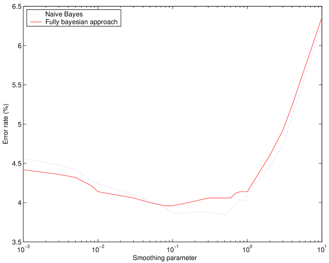
Figure 1: Error rate as a function of $\lambda$.

Both approaches yield very comparable results. Naive Bayes seems to outperform the fully Bayesian approach for larger values of the smoothing parameter while the converse is true for smaller values. However, the performance is very similar, since the largest difference between the scores of both approaches is around $0.2\%$, corresponding to one text only in our test corpus composed by 500 documents for each fold.

We also tested on other common text classification benchmarks such as 20-Newsgroups (Lang, 1995) and Spam Assassin (Mason, 2002), and tried to change the number of documents or size of vocabulary and the difference never gets statistically significant. Given that the naive Bayes classifier is known to perform worse than state-of-the-art classification methods (Yang and Liu, 1999; Sebastiani, 2002), the fully Bayesian classifier does not seem to be promising for supervised text classification tasks. This is not surprising as the conditions (i) and (ii) discussed above are nearly satisfied in this context.

We now turn to the unsupervised clustering case, where the fully Bayesian perspective will prove more useful.

4 Unsupervised Inference

When document labels are unknown, the multinomial mixture model may be used to create a probabilistic clustering rule. In this context, the performance of the method is more difficult to assess. We therefore start this section with a discussion of our evaluation protocol (Section 4.1). For estimating the parameters of the model, we first consider the most widespread approach, which is based on the use of the Expectation-Maximization (EM) algorithm. It turns out that in the context of large scale text processing applications, this basic approach is plagued by an acute sensitivity to initialization conditions. We then consider alternative estimation procedures, based either on heuristic considerations aimed at reducing the variability of the EM estimates (Section 4.4) or on the use of various forms of Markov chain Monte Carlo simulations (Section 4.5) and show that these techniques can yield less variable estimates.

4.1 Experimental Framework

We will use the same fraction of the Reuters corpus as in Section 3. As will be discussed below, initialization of the EM algorithm does play a very important role in obtaining meaningful document clusters. To evaluate the performance of the model, one option is to look at the value of the log-likelihood at the end of the learning procedure. However, this quantity is only available on the training data and does not tell us anything about the generalization abilities of the model. A more meaningful measure, commonly used in text applications, is the perplexity. Its expression on the test data is:

$$\widehat{\mathcal{P}}^{\star}=\exp[-\frac{1}{l^{\star}}\sum_{d=1}^{n^{\star}_{D}}\log(\sum_{t=1}^{{n_{T}}}\alpha_{t}\prod_{w=1}^{{n_{W}}}\beta_{wt}^{C_{wd}^{\star}})]\,.$$

It quantifies the ability of the model to predict new documents. The normalization by the total number of word occurrences $l^{\star}$ in the test corpus $C^{\star}$ is conventional and used to allow comparison with simpler probabilistic models, such as the unigram model, which ignores the document level. For the sake of coherence, we will also compute perplexity, rather than log-likelihood, on the training data: their variations are in fact equivalent as they are identical up to the normalization constant and the exponential function.

A second indicator, also computable on the training and test data, is obtained by comparing the cooccurrences of documents between “equivalent” clusters in two clusterings. To do so, we must have a way to establish the best mapping between clusters in two different clusterings. Provided that the two clusterings have the same size, this can be done with the so-called Hungarian method (Kuhn, 1955; Frank, 2004), an algorithm for computing the best weighted matching in a bi-partite graph. The complexity of this algorithm is cubic in the number of clusters involved. Once a one-to-one mapping between clusters is established, the score we consider is the ratio of documents for which the two clusterings “agree”, that is, which lie into clusters that are mapped by the Hungarian method. (Lange et al., 2004) describes in more detail how this method can be used to evaluate clustering algorithms.

A limitation of the evaluation with the Hungarian method is that it is not suited to compare two soft clusterings with different number of classes and especially the cases where one class in clustering $A$ is split into two classes in clustering $B$. There exist other information-based measures built, such as the Relative Information Gain, that do not suffer from this limitation but present other drawbacks, such as undesirable behaviors for distributions close to equiprobability. We do not consider those here, as cooccurrence scores obtained with the Hungarian method are easier to interpret (see Rigouste et al., 2005a, for results on the same database quantified in terms of mutual information).

4.2 Expectation-Maximization algorithm

In an unsupervised setting, the maximum a posteriori estimates are obtained by maximizing the posterior distribution given in (2). The resulting maximization program is unfortunately not tractable. It is however possible to devise an iterative estimation procedure, based on the Expectation-Maximization (EM) algorithm. Denoting respectively by $\alpha^{\prime}$ and $\beta^{\prime}$ the current estimates of the parameters and by $T_{d}$ the latent (unobservable) theme of document $d$, it is straightforward to check that each iteration of the EM algorithm updates the parameters according to:

$$\operatorname{P}(T_{d}=t|C;\alpha^{\prime},\beta^{\prime})=\frac{\alpha_{t}^{\prime}\prod_{w=1}^{{n_{W}}}\beta_{wt}^{\prime C_{wd}}}{\sum_{t^{\prime}=1}^{{n_{T}}}\alpha_{t^{\prime}}^{\prime}\prod_{w=1}^{{n_{W}}}\beta_{wt^{\prime}}^{\prime C_{wd}}}$$ (9)

$$\alpha_{t}\propto\lambda_{\alpha}-1+\sum_{d=1}^{{n_{D}}}\operatorname{P}(T_{d}=t|C;\alpha^{\prime},\beta^{\prime})$$ (10)

$$\beta_{wt}\propto\lambda_{\beta}-1+\sum_{d=1}^{{n_{D}}}C_{wd}\operatorname{P}(T_{d}=t|C;\alpha^{\prime},\beta^{\prime})$$ (11)

where the normalization factors are determined by the constraints:

$$\left\{\begin{array}[]{ll}\sum_{t=1}^{{n_{T}}}\alpha_{t}=1&\\ \sum_{w=1}^{{n_{W}}}\beta_{wt}=1&\mbox{for $t$ in $\{1,\dots,{n_{T}}\}$}.\end{array}\right.$$

In the remainder of this section, we present the results of a series of experiments based on the use of the EM algorithm. We first discuss issues related to the initialization strategy, before empirically studying the influence of the smoothing parameters. The main findings of these experiments is that the EM estimates are very unstable and vary greatly depending on the initial conditions: this outlines a limitation of the EM algorithm, i.e. its difficulty to cope with the very high number of local maxima in high dimensional spaces. In comparison, the influence of the smoothing parameter is moderate, and its tuning should not be considered a major issue.

4.2.1 Initialization

It is important to realize that the EM algorithm allows to go back and forth between the values of the parameters $\alpha$ and $\beta$ and the values of the posterior probabilities $\operatorname{P}(T_{d}=t|C;\alpha,\beta)$ using formulas (9), (10) and (11). Therefore, the EM algorithm can be initialized either from the E-step, providing initial values for the parameters, or from the M-step, providing initial values for the posterior probabilities (that is, roughly speaking, an initial soft clustering). There are various reasons to prefer the second solution:

• Initializing $\beta$ requires to come up with a reasonable value for a very large number of parameters. A random initialization scheme is out of the question, as it almost always yields very unrealistic values in the parameter space; an alternative would be to consider small deviations from the unigram word frequencies: it is however unclear how large these deviations should be.

• Initializing on posterior probabilities can be done without any knowledge of the model: for instance, it can be performed without knowing the vocabulary size. Section 4.4 will show why this is a desirable property.

Consequently, in the rest of this article, we will only consider initialization schemes that are based on the posterior theme probabilities associated with each document. A good option is to make sure that, initially, all clusters significantly overlap. Our “Dirichlet” initialization consists in sampling, independently for each document, an initial (fictitious) configuration of posterior probabilities from an exchangeable Dirichlet distribution. In practice, we used the uniform distribution over the ${n_{T}}$-dimensional probability simplex (Dirichlet with parameter 1). As the EM iterations tend to amplify even the smaller discrepancies between the components, the variability of the final estimates was not significantly reduced when initializing from exchangeable Dirichlet distributions with lower variance (ie., higher parameter value).

To get an idea about the best achievable performance, we also used the Reuters categories as initialization. We establish a one-to-one mapping between the mixture components and the Reuters categories, setting for each document the initial posterior probability in (9) to 1 for the corresponding theme. Figure 2 displays the corresponding perplexity on the training and test sets as a function of the number of iterations. Results are averaged over 10 folds and 30 initializations per fold and are represented with box-and-whisker curves: the boxes being drawn between the lower and upper quartiles, the whiskers extending down and up to $\pm 1.5$ times the interquartile range (the outliers, a couple of runs out of the 300, have been removed).

The variations are quite similar on both (training and test) datasets. The main difference is that test perplexity scores are worse than training perplexity scores. This classical phenomenon is an instance of overfitting. Due to the way the indexing vocabulary is selected (discarding words that do not occur in the training data), this effect is not observed for the unigram model.

The most striking observation is that the gap between both initialization strategies is huge. With the Dirichlet initialization, we are able to predict the word distribution more accurately than with the unigram model but much worse than with the somewhat ideal initialization. This gap is also patent for the cooccurrence scores with a final ratio of 0.95 for the “Reuters categories” initialization and an average around 0.6 for the Dirichlet initialization on test data.

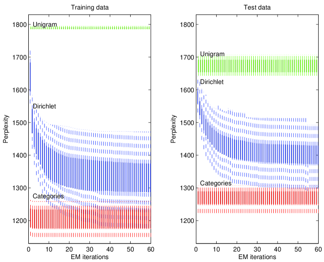
Figure 2: Evolution of Perplexity on training and test data over the EM iterations.

Given that the Dirichlet initialization involves random sampling, it is worth checking how the performance change from one run to another. We report in Figure 3 the values of training perplexity and test cooccurrence scores for various runs on the first fold. As can be seen more clearly on this figure, the variability from one initialization to another is very high for both measures: for instance, the cooccurrence score varies from about $0.4$ to more than $0.7$. This variability is a symptom of the inability of the EM algorithm to avoid being trapped in one of the abundant local maxima which exist in the high-dimensional parameter space.

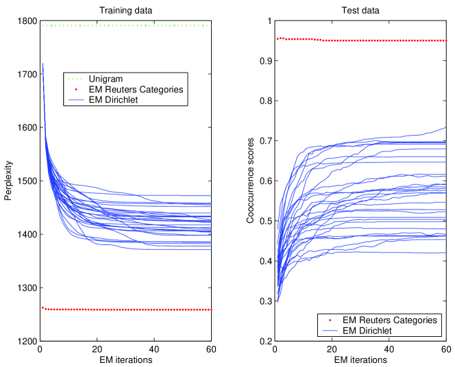
Figure 3: Evolution of Perplexity and Cooccurrence scores over the EM iterations for different Dirichlet initializations for the first fold.

4.2.2 Influence of the smoothing parameter

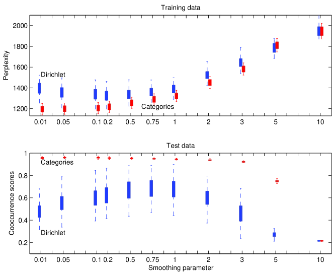
Figure 4: Evolution of training perplexity and test cooccurrence scores over the smoothing parameter $\lambda_{\beta}-1$.

Figure 4 depicts the influence of the smoothing parameter $\lambda_{\beta}-1$ in terms of perplexity and cooccurrence scores. We do not consider here the influence of $\lambda_{\alpha}-1$, which is, in our context, always negligible with respect to the sum over documents of the themes posterior probabilities. For the Reuters categories initialization, there is almost no difference in perplexity scores for small values of $\lambda_{\beta}-1$ (i.e. when $\lambda_{\beta}-1\leq 0.2$). The performance degrades steadily for larger values, showing that some information is lost, probably in the set of rare words (since smoothing primarily concerns parameters corresponding to very few occurrences). Similarly, for the Dirichlet initialization, the variations in perplexity are moderate for smoothing values in the range $0.01$ to $1$, yet there is a more distinguishable optimum, around $0.2$. Using some prior information about the fact that word probabilities should not get too small helps to fit the distribution of new data, even for words that are rarely (or even never) seen in association with a given theme.

These observations are confirmed by the observation of the test cooccurrence scores. First, except when using very large ($5$ or more) values of the smoothing parameters, which yields a serious drop in performance, the categorization accuracy is rather insensitive to the smoothing parameter for the Reuters categories initialization. Of more practical interest however is the behavior for the Dirichlet initialization: the variations in performance are again moderate, with however a higher optimum value around $0.75$. A possible explanation of this observation that more smoothing improves categorization capabilities (even if it slightly degrades distribution fit) is that the model is so coarse and the data so sparse that only quite frequent words are helpful in categorizing; the other words are essentially misleading, unless properly initialized. This suggests that removing rare words from the vocabulary could improve the classification accuracy.

All in all, changing the values of $\lambda_{\alpha}-1$ and $\lambda_{\beta}-1$ does not make the most important differences in the results, as long as they remain within reasonable bounds. Thus, in the rest of this article, we set them respectively to $0$ and $0.1$.

4.3 EM and deterministic clustering

A somewhat unexpected property of the multinomial mixture model is that a huge fraction of posterior probabilities (that a document belongs to a given theme) is in fact very close to $0$ or $1$. Indeed, when starting from the Reuters categories, the proportion of texts classified in only one given theme (that is, with probability one, up to machine precision) is almost 100%. As we start from the opposite point of “extreme fuzziness”, this effect is not as strong with the Dirichlet initialization. Nevertheless, after the fifth iteration, more than 90% of the documents are categorized with almost absolute certainty. This suggests that in the context of large-dimensional textual databases, the multinomial mixture model in fact behaves like a deterministic clustering algorithm.

This intuition has been experimentally confirmed as follows, implementing a “hard” (deterministic) clustering version of the EM algorithm, in which the E-step uses deterministic rather than probabilistic theme assignments. This algorithm can be seen as an instance of a $K$-means algorithm, where the similarity between a text $d\in\{1,\ldots,n_{D}\}$ and theme (or cluster) $t\in\{1,\ldots,{n_{T}}\}$ is computed as:

$$\operatorname{dist}(d,t)=-\sum_{w=1}^{{n_{W}}}C_{wd}\log(\beta_{wt})+\log\alpha_{t}$$

Up to a constant term, which only depends on the document, the first term is the Bregman divergence (Banerjee et al., 2005) between a theme specific distribution and the document, viewed as an empirical probability distribution over words. This measure is computed for every document and every theme, and each document is assigned to the closest theme. The reestimation of the parameters $\beta_{wt}$ is still performed according to (11), where the posterior “probabilities” are either $0$ or $1$. The weight $\alpha_{t}$ simply becomes the proportion of documents in theme $t$ and $\beta_{wt}$ the ratio of the number of occurrences of $w$ in theme $t$ over the total number of occurrences in documents in theme $t$.

$$\alpha_{t} = \frac{\#\{d:T_{d}=t\}}{n_{D}}$$

$$\beta_{wt} = \frac{\sum_{\{d:T_{d}=t\}}C_{wd}}{\sum_{w=1}^{n_{W}}\sum_{\{d:T_{d}=t\}}C_{wd}}$$

This algorithm was applied to the same dataset, with the same initialization procedures as above. At the end of each iteration, we compute the cooccurrence score between the probabilistic clustering produced by EM and the hard clustering produced by this version of K-means.

• With the Reuters Categories initialization, the cooccurrence score between both clusterings is $1$ after one iteration.

• With the Dirichlet initialization, the score between the soft and hard clustering quickly converges to $1$ and is greater than $0.99$ after five iterations.

In both cases, the outputs of the probabilistic and hard methods become indiscernible after very few iterations. We believe that this behavior of EM can be partly explained by the large dimensionality of the space of documents. This assumption has been verified with experiments on artificially simulated datasets, which are not reported here for reason of space.

4.4 Improving EM via dimensionality reduction

In this section, we push further our intuition that removing rare words should improve the performance of the EM algorithm and should alleviate the variability phenomenons observed in the previous section. After studying the effect of dimensionality reduction, we propose a novel strategy based on iterative inference.

4.4.1 Adjusting the Vocabulary Size

Having decided to ignore part of the vocabulary, the next question is whether we should rather discard the rare words or the frequent words. In this section, we experimentally assess these strategies, by removing consecutively tens, hundreds and thousands of terms from the indexing vocabulary. The words that are discarded are simply removed from the count matrix. Results presented in Figure 5 suggest that the performance of the model with the Dirichlet initialization can be substantially improved by keeping a limited number of frequent words (900 out of 40,000).

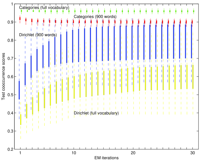
Figure 5: Evolution of test cooccurrence scores over the EM iterations with a vocabulary of size 900.

When varying the size of the vocabulary, perplexity measurements are meaningless, as the reduction of dimensionality has an impact on perplexity which is hard to distinguish from the variations due to a possible better fit of the model. The test cooccurrence score, on the other hand, is meaningful even when with varying vocabulary sizes. Figure 6 plots the test cooccurrence scores at the end of the 30th EM iteration as a function of the vocabulary size. For the sake of readability, the scale of the x-axis is not regular but rather focuses on the interesting parts: the interval between $100$ and $3,000$ words, which corresponds to keeping only the frequent words, and the region above $40,000$ (out of a complete vocabulary of $43,320$ forms), which corresponds to keeping only the rare words. This choice is motivated by the well-known fact that most of the occurrences (and therefore most of the information) are due to the most frequent words: for instance, the $3,320$ most frequent words account for about $75\%$ of the total number of occurrences.

The upper graph in Figure 6 shows that removing rare words always hurts when using the Reuters categories initialization. In contrast, with the Dirichlet initialization, considering a reduced vocabulary (between $300$ and $3,000$ words) clearly improves the performance. The somewhat optimal size of the vocabulary, as far as this specific measure is concerned, seems to be around $1,000$. Also importantly, the performance seems much more stable when using reduced versions of the vocabulary, an effect we did not manage to achieve by adjusting the smoothing parameter. We will come back to this in the next section. It suffices to say here that the best score obtained with the Dirichlet initialization is still far behind the performance attained with the Reuters categories initialization. This agrees with our previous observation that even the rarest word are informative, when properly initialized.

Less surprisingly, on the lower portion of the graph, one can see that removing the frequent words almost always hurts the performance. It is only in the case of the Reuters categories initialization that the removal of the $100$ most frequent words actually yields a slight improvement of performance. Then the score steadily decreases with the removal of frequent words. The score is almost $0.2$ (random agreement) with $20,000$ rare words, which is not surprising, as, in this case, the vocabulary mainly contains words occurring only once (so-called hapax legomena) in the corpus, reducing texts to at most a dozen of terms.

Figure 6: Evolution of test cooccurrence scores over the size of vocabulary with two different strategies: discarding most rare words or discarding most frequent words.

To sum-up, there are two important lessons to draw from these experiments:

• Reducing the dimensionality (vocabulary size) while the number of examples (size of the corpus) remains the same helps the inference procedure;

• Using a reduced vocabulary allows to significantly reduce the variability of the parameter estimates.

We now consider ways to use these remarks to improve our estimation procedure.

4.4.2 Iterative estimation procedures

In this section, we look for ways to reduce the variability of the clustering: our main goal here being that an end-user should get sufficiently reliable results without having to run the program several times and/or to worry about evaluation measures.

Incremental vocabulary

The first idea is to take advantage of our previous observations that reducing the dimension of the problem seems to make the EM algorithm less dependent on initial conditions. This suggests to obtain robust posterior probabilities using a reduced vocabulary, and to use them for initializing new rounds of EM iterations, with a larger vocabulary. Proceeding this way allows us to circumvent the problem of initializing the $\beta$ parameters corresponding to rare words, as we start from the other step of the algorithm (the M-step). When the vocabulary size is increased, the probabilities associated with new words are implicitly initialized on their average count in the corpus, weighted by the current posterior probabilities.This iterative procedure has the net effect of decomposing the inference process into several steps, each being sufficiently stable to yield estimates having both a small variance and good generalization performance.

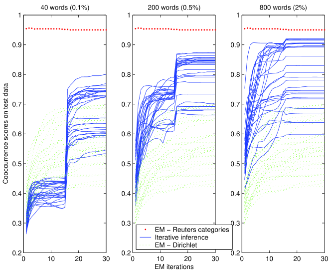
Figure 7: Evolution of cooccurrence scores on test data with different vocabulary sizes. The first 15 iterations are conducted on reduced vocabularies (the size of which is reported on top the figures), while the last 15 are use the complete vocabulary.

Figure 7 displays the results of the following set of experiments: we perform 15 EM iterations with a reduced vocabulary, save the values of posterior probabilities at the end of the 15th iteration, and use these values to initialize another round of 15 EM iterations, using the full vocabulary. Our earlier results obtained using the full vocabulary are also reported for comparison. The influence of the initial vocabulary size is important: as it is increased, the maximal score gets somewhat better but the results are more variable.

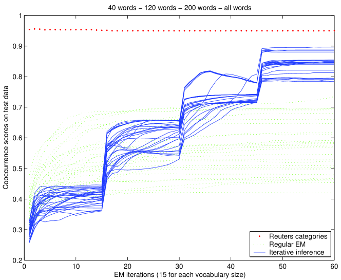
Figure 8: Evolution of cooccurrence scores over the different steps of an iterative algorithm (30 runs on the same fold).

These results can be improved by making the estimation process more gradual, thus reducing the variability of our estimates. Such experiments are reported in Figure 8 where we use four different steps. Proceeding this way, both the maximal and minimal scores lie within an acceptable range of performance. It is clear from these experiments that the choice of the successive sizes of vocabulary is particularly difficult, being a tight compromise between quality and stability. It remains to be seen how to devise a principled approach for finding such appropriate vocabulary increments.

Multiple restarts

Another usual approach in optimization problems where the large number of local optima yields unstable results is to perform multiple restarts and pick up the best run according to some criterion. From this point of view, a sensible strategy is to choose the vocabulary size yielding the best maximum performance (for instance, Figure 7 suggests that starting with $800$ words is a reasonable choice), run several trials and select the parameter set yielding the best cooccurrence score on the test data. For lack of this information (as would be the case in a real-life study, where no reference clustering is available), a legitimate question to ask is whether the training perplexity could be used instead as a reliable indicator of the quality of parameter settings. The answer is positive, as is shown in Figure 9.

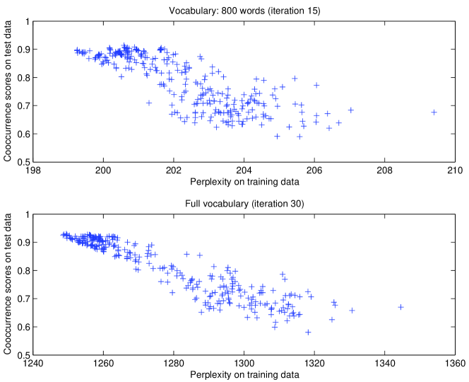
Figure 9: Correlation between training perplexity and test cooccurrence scores.

This figure reports results of the following experiments: after 15 EM iterations using a reduced vocabulary of $800$ words, we consider the complete vocabulary for another 15 additional EM iterations. Training set perplexity is computed at the end of iteration 15 and at the end of iteration 30. These measurements are repeated 30 times for each of the 10 folds. The test cooccurrence scores (somewhat representing the quality of clustering) are plotted as a function of this training perplexity in Figure 9. There is a clear inverse correlation, especially in the area of the best runs (low perplexity values–large cooccurrence scores) we are interested in. Selecting the run with lowest perplexity yields acceptable performance in both cases and the correlation is even stronger on the full vocabulary (it is therefore worth performing 15 more iterations with all the words).

In summary, we have presented in this section two inference strategies which significantly improve over a basic implementation of the EM algorithm:

• split the vocabulary in several bins (at least 4) based on frequency; run EM on the smallest set and iteratively add words and rerun EM.

• discard rare words, run several rounds of EM iterations, keep the run yielding the best training perplexity.

(Rigouste et al., 2005b) reports experiments which show that these strategies can be combined, yielding improved estimates of the parameters.

4.5 Gibbs sampling algorithm

In this section, we experiment with an alternative inference method, Gibbs sampling. The first subsection presents the results obtained with the most “naive” Gibbs sampling algorithm, which is then compared with a Rao-Blackwellized version relying on the integrated formula introduced in (7).

4.5.1 Sampling from the EM formulas

To apply Gibbs sampling, we first need to identify sets of variables whose values may be sampled from their joint conditional distribution given the other variables. In our case, the most straightforward way to achieve this is to use the EM update equations (9), (10), (11). Hence, we may repeatedly:

• sample a theme indicator in $\{1,\dots,{n_{T}}\}$ for each document from a multinomial distribution whose parameter is given by the posterior probability that the document belongs to each of the themes;

• sample values for $\alpha,\beta$ which, conditionally upon the theme indicators, follow Dirichlet distributions;

• compute new posterior probabilities according to (9).

Figure 10 displays the evolution of the training perplexity and the test cooccurrence score for 200 runs of the Gibbs sampler (ran for 10,000 iterations on one fold), compared to the regular EM algorithm and the iterative inference method described in Section 4.4. The performance varies greatly from one run to another and, occasionally, large changes occur during a particular run. This behavior suggests that, in this context, the Gibbs sampler does not really attain its objective and gets trapped, like the EM algorithm, in local modes. Hence, one does not really sample from the actual posterior distribution but rather from the posterior restricted to a “small” subset of the space of latent variables and parameters. Results in terms of perplexity and cooccurrence scores are in the same ballpark as those obtained with the EM algorithm, several levels below the ones obtained with the ad-hoc inference method of Section 4.4.2.

Figure 10: Evolution of perplexity and cooccurrence scores over the EM–Gibbs Sampling iterations.

4.5.2 Rao-Blackwellized Gibbs Sampling

There is actually no need to simulate the parameters $\alpha$ and $\beta$, as they can be integrated out when considering the conditional distribution of a single theme given in (7). We then obtain an estimate of the distribution of the themes $T$ of all documents by applying the Gibbs sampling algorithm to simulate, in turn, every latent theme $T_{d}$, conditioned on the theme assignment of all other documents. This strategy, which aims at reducing the number of dimensions of the sampling space, is known as Rao-Blackwellized sampling, and often produces good results (Robert and Casella, 1999). Note that if the document $d$ is one word long, this approach is identical to the Gibbs sampling algorithm described in (Griffiths and Steyvers, 2002) for the LDA model (using the identity $\Gamma(a+1)=a\Gamma(a)$).

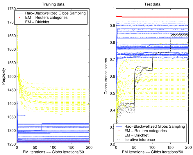
Figure 11: Evolution of the different measures for Rao-Blackwellized Gibbs Sampling

Figure 11 displays the training perplexity and the test cooccurrence scores for 30 independent random initializations of the Gibbs sampler, compared to the same references as in the previous section. We plot results obtained on 200 samples, each corresponding to 10,000 complete cycles on one fold. The Gibbs sampler outperforms the basic EM algorithm for almost all runs. Its performance is in the same range as the iterative method, albeit much more variable (the cooccurrence score lies in the range 70% to 95%). The sampler trajectories also suggest that the Gibbs sampler is not really irreducible in this context and only explores local modes.

This alternative implementation of the Gibbs sampling procedure is obviously much better than our first, arguably more naive, attempt: not only does it yield consistently better performance, but it is also much faster. Thanks to the tabulation of the Gamma function, the deterministic computations needed for both versions of the sampler are comparable. But the Gibbs sampler based on the EM formulas requires generating ${n_{T}}+1$ Dirichlet samples (with respective dimensions ${n_{W}}$ and ${n_{T}}$) for a rough total of approximately ${n_{W}}{n_{T}}$ Gamma distributed variables for the M-step, and ${n_{D}}$ samples from ${n_{T}}$-dimensional discrete distributions for the E-step. In comparison, the Rao-Blackwellized Gibbs sampling only requires ${n_{D}}$ ${n_{T}}$-dimensional samples from discrete distributions. The difference is significant: our C-coded implementation of the latter algorithm runs 20 times faster than the vanilla Gibbs sampler.

5 Conclusion

In this article, we have presented several methods for estimating the parameters of the multinomial mixture model for text clustering. A systematic evaluation framework based on various measures allowed us to understand the discrepancy between the performance typically obtained with a single run of the EM algorithm and the best scores we could possibly attain when initializing on a somewhat ideal clustering.

Based on the intuition that the high dimensionality incurred by a “bag-of-word” representation of texts is directly responsible for this undesirable behavior of the EM algorithm, we have analyzed the benefits of reducing the size of the vocabulary and suggested a heuristic inference method which yields a significant improvement in comparison to the basic application of the EM algorithm.

We have also investigated the use of Gibbs sampling, and proposed two different approaches. The Rao-Blackwellized version, which takes advantage of analytic marginalization formulas clearly outperforms the other, more straightforward, implementation. Performance obtained with Gibbs sampling are close to the ones obtained with the iterative inference method, albeit more dependent on initial conditions.

Altogether, these results clearly highlight the too often overlooked fact that the inference of probabilistic models in high-dimensional spaces, as is typically required for text mining applications, is prone to an extreme variability of estimators.

This work is currently extended in several directions. Further investigations of the multinomial mixture model are certainly required, notably aiming at (i) analyzing its behavior when used with very large numbers (several hundreds) number of themes, as in (Blei et al., 2002); (ii) investigating model selection procedures to see how they can help discover the proper number of themes; (iii) reducing the overall complexity of the training: both the EM-based and the Gibbs sampling algorithm require to iterate over each document, an unrealistic requirement for very large databases.

Another promising line of research is to consider alternative models: the multinomial mixture model can be improved in multiple ways: (i) its modeling of the count matrix is unsatisfactory, especially as it does not take in account typical effects of word occurrence distributions (Church and Gale, 1995; Katz, 1996): this suggests to consider alternative, albeit more complex models of the counts; (ii) the one document-one theme assumption is also restrictive, pleading for alternative models such as LDA (Blei et al., 2002) or GAP (Canny, 2004): preliminary experiments with the former model however suggest that it might be faced with the same type of variability issues as the multinomial mixture model (Rigouste et al., 2006).

References

- Banerjee et al. [2005] A. Banerjee, S. Merugu, I. S. Dhillon, and J. Ghosh. Clustering with Bregman divergences. Journal of Machine Learning Research, 6:1705–1749, 2005.
- Blei et al. [2002] D. M. Blei, A. Y. Ng, and M. I. Jordan. Latent Dirichlet allocation. In T. G. Dietterich, S. Becker, and Z. Ghahramani, editors, Advances in Neural Information Processing Systems (NIPS), volume 14, pages 601–608, Cambridge, MA, 2002. MIT Press.
- Buntine and Jakulin [2004] W. Buntine and A. Jakulin. Applying discrete PCA in data analysis. In M. Chickering and J. Halpern, editors, Proceedings of the 20th Conference on Uncertainty in Artificial Intelligence (UAI’04), pages 59–66. AUAI Press, 2004.
- Canny [2004] J. F. Canny. GAP: A factor model for discrete data. In Proceedings of the ACM Conference on Information Retrieval (SIGIR), Sheffield, England, 2004.
- Church and Gale [1995] K. W. Church and W. A. Gale. Poisson mixtures. Journal of Natural Language Engineering, 1(2):163–190, 1995.
- Deerwester et al. [1990] S. C. Deerwester, S. T. Dumais, T. K. Landauer, G. W. Furnas, and R. A. Harshman. Indexing by latent semantic analysis. Journal of the American Society of Information Science, 41(6):391–407, 1990.
- Frank [2004] A. Frank. On Kuhn’s Hungarian method - a tribute from Hungary. Technical Report TR-2004-14, Egerváry Research Group, Budapest, 2004. URL http://www.cs.elte.hu/egres/www/tr-04-14.html.
- Griffiths and Steyvers [2002] T. L. Griffiths and M. Steyvers. A probabilistic approach to semantic representation. In Proceedings of the 24th Annual Conference of the Cognitive Science Society, 2002.
- Halkidi et al. [2001] M. Halkidi, Y. Batistakis, and M. Vazirgiannis. On clustering validation techniques. Intelligent Information Systems Journal, 12(2–3):107–145, 2001.
- Hofmann [2001] T. Hofmann. Unsupervised learning by probabilistic latent semantic analysis. Machine Learning Journal, 42(1):177–196, 2001.
- Jain et al. [1999] A. K. Jain, M. N. Murphy, and P. Flynn. Data clustering: a review. ACM Computing surveys, 31(3):264–323, 1999.
- Katz [1996] S. M. Katz. Distribution of content words and phrases in text and language modelling. Journal of Natural Language Engineering, 2(1):15–59, 1996.
- Kuhn [1955] H. Kuhn. The Hungarian method for the assignment problem. Naval Research Logistic Quarterly, 2:83–97, 1955.
- Lang [1995] K. Lang. NewsWeeder: Learning to filter netnews. In Proceedings of the 12th ICML International Conference on Machine Learning, pages 331–339, 1995.
- Lange et al. [2004] T. Lange, V. Roth, M. L. Braun, and J. M. Buhmann. Stability-based validation of clustering solutions. Neural Computation, 16(6):1299–1323, 2004.
- Lewis [1998] D. D. Lewis. Naive (Bayes) at forty: The independence assumption in Information Retrieval. In C. Nédellec and C. Rouveirol, editors, Proceedings of ECML-98, 10th European Conference on Machine Learning, pages 4–15, Chemnitz, DE, 1998. Springer Verlag, Heidelberg, DE.
- Mason [2002] J. Mason. SpamAssassin corpus, 2002. URL http://spamassassin.apache.org/publiccorpus/.
- McCallum and Nigam [1998] A. McCallum and K. Nigam. A comparison of event models for Naive Bayes text classification. In AAAI-98 Workshop on Learning for Text Categorization, 1998.
- Minka [2003] T. P. Minka. Estimating a Dirichlet distribution. Technical report, Carnegie Mellon University, 2003. URL http://www.stat.cmu.edu/~minka/papers/dirichlet/.
- Mosimann [1962] J. E. Mosimann. On the compound multinommial distribution, the multivariate -distribution, and correlations among proportions. Biometrika, 49(1–2):65–82, 1962.
- Nigam et al. [2000] K. Nigam, A. K. McCallum, S. Thrun, and T. M. Mitchell. Text classification from labeled and unlabeled documents using EM. Machine Learning, 39(2/3):103–134, 2000.
- Reuters [2000] Reuters. Reuters corpus, 2000. URL http://about.reuters.com/researchandstandards/corpus/.
- Rigouste et al. [2005a] L. Rigouste, O. Cappé, and F. Yvon. Evaluation of a probabilistic method for unsupervised text clustering. In Proceedings of the International Symposium on Applied Stochastic Models and Data Analysis (ASMDA), Brest, France, 2005a.
- Rigouste et al. [2005b] L. Rigouste, O. Cappé, and F. Yvon. Inference for probabilistic unsupervised text clustering. In Proceedings of the IEEE Workshop on Statistical Signal Processing (SSP’05), Bordeaux, France, 2005b.
- Rigouste et al. [2006] L. Rigouste, O. Cappé, and F. Yvon. Quelques observations sur le modèle LDA. In J.-M. Viprey, editor, Actes des IXe JADT, pages 819–830, Besançon, 2006.
- Robert and Casella [1999] C. P. Robert and G. Casella. Monte Carlo Statistical Methods. Springer, 1999.
- Sebastiani [2002] F. Sebastiani. Machine learning in automated text categorization. ACM Computing Surveys, 34(1):1–47, 2002.
- Shahnaz et al. [2006] F. Shahnaz, M. W. Berry, V. P. Pauca, and R. J. Plemmons. Document clustering using nonnegative matrix factorization. Information Processing and Management, 42(2):373–386, 2006.
- Vinokourov [2002] A. Vinokourov. Why nonnegative matrix factorization works well for text information retrieval. URL http://citeseer.ist.psu.edu/458322.html. Preprint, 2002.
- Vinot and Yvon [2003] R. Vinot and F. Yvon. Improving Rocchio with weakly supervised clustering. In Proceedings of the European Conference on Machine Learning (ECML), pages 456–467, Cavtat-Drubrovnick, Croatie, 2003.
- Yang and Liu [1999] Y. Yang and X. Liu. A re-examination of text categorization methods. In 22nd Annual International SIGIR, pages 42–49, 1999.