On the Efficiency of Strategies for Subdividing Polynomial Triangular Surface Patches

Abstract. In this paper, we investigate the efficiency of various strategies for subdividing polynomial triangular surface patches. We give a simple algorithm performing a regular subdivision in four calls to the standard de Casteljau algorithm (in its subdivision version). A naive version uses twelve calls. We also show that any method for obtaining a regular subdivision using the standard de Casteljau algorithm requires at least $4$ calls. Thus, our method is optimal. We give another subdivision algorithm using only three calls to the de Casteljau algorithm. Instead of being regular, the subdivision pattern is diamond-like. Finally, we present a “spider-like” subdivision scheme producing six subtriangles in four calls to the de Casteljau algorithm.

1 Introduction

In this paper, we investigate the efficiency of various strategies for subdividing polynomial triangular surface patches. Subdivision methods based on a version of the de Casteljau algorithm splitting a control net into control subnets (see Farin [5]) were investigated by Goldman [11], Boehm and Farin [2], Böhm [4], and Seidel [16] (see also Boehm, Farin, and Kahman [3], and Filip [8]). However, except for Böhm [4], these papers are not particularly concerned with minimizing the number of calls to the standard de Casteljau algorithm. Furthermore, some of these papers (notably Goldman [11]) use a version of the de Casteljau algorithm computing a $5$-dimensional simplex of polar values, which is more expensive than the standard $3$-dimensional version. In this paper, we give a simple algorithm performing a regular subdivision in four calls to the standard de Casteljau algorithm (in its subdivision version). A naive version uses twelve calls. We also show that any method for obtaining a regular subdivision using the standard de Casteljau algorithm requires at least $4$ calls. Thus, our method is optimal. We give another subdivision algorithm using only three calls to the de Casteljau algorithm. Instead of being regular, the subdivision pattern is diamond-like. Finally, we present a “spider-like” subdivision scheme producing six subtriangles in four calls to the de Casteljau algorithm. Some familiarity with affine spaces and affine maps is assumed. Details can be found in Farin [7], Berger [1], or Gallier [9].

2 The Polar Form Approach to Polynomial Triangular Surface Patches

The deep reason why polynomial triangular surface patches can be effectively handled in terms of control points is that multivariate polynomials arise from multiaffine symmetric maps (see Ramshaw [14], Farin [7, 6], Hoschek and Lasser [12], or Gallier [9]). Denoting the affine plane $\mathbb{R}^{2}$ as ${\cal P}$, traditionally, a polynomial surface in $\mathbb{R}^{n}$ is a function $F\colon{\cal P}\rightarrow\mathbb{R}^{n}$, defined such that

$$\openup 3.0pt\halign to=0.0pt{\hfil$\displaystyle{#}$&$\displaystyle{{}#}$\hfil&\llap{$#$}\cr x_{1} &= F_{1}(u,v),\cr\ldots&= \ldots\cr x_{n} &= F_{n}(u,v),\cr}$$

for all $u,v\in\mathbb{R}$, where $F_{1}(U,V),\ldots,F_{m}(U,V)$ are polynomials in $\mathbb{R}[U,V]$. Given a natural number $m$, if each polynomial $F_{i}(U,V)$ has total degree $\leq m$, we say that $F$ is a polynomial surface of total degree $m$. The trace of the surface $F$ is the set $F({\cal P})$.

Now, given a polynomial surface $F$ of total degree $m$ in some affine space ${\cal E}$ (typically $\mathbb{R}^{3}$), there is unique symmetric and multiaffine map $f\colon{\cal P}^{m}\rightarrow{\cal E}$ such that

$$F(u,v)=f(\underbrace{(u,v),\ldots,(u,v)}_{m}),$$

for all $(u,v)\in{\cal P}$. The symmetric and multiaffine map $f$ associated with $F$ is called the polar form of $F$.

The above result is not hard to prove. Using linearity, it is enough to deal with a single monomial. Given a monomial $U^{h}V^{k}$, with $h+k=d\leq m$, it is easily shown that the symmetric multiaffine $f$ form corresponding to $U^{h}V^{k}$ is given

$$f((u_{1},v_{1}),\ldots,(u_{m},v_{m}))=\frac{h!k!(m-(h+k))!}{m!}\>\sum_{\scriptstyle I\cup J\subseteq\{1,\ldots,m\}\atop{\scriptstyle I\cap J=\emptyset\atop\scriptstyle\mathrm{card}{(I)}=h,\,\mathrm{card}{(J)}=k}}\biggl{(}\prod_{i\in I}u_{i}\biggr{)}\biggl{(}\prod_{j\in J}v_{j}\biggr{)}.$$

Recall that a map $f\colon\mathbb{R}^{d}\rightarrow\mathbb{R}^{n}$ is affine if

$$f((1-\lambda)a+\lambda b)=(1-\lambda)f(a)+\lambda f(b),$$

for all $a,b\in\mathbb{R}^{d}$, and all $\lambda\in\mathbb{R}$. A map $f\colon\underbrace{\mathbb{R}^{d}\times\cdots\times\mathbb{R}^{d}}_{m}\rightarrow\mathbb{R}^{n}$ is multiaffine if it is affine in each of its arguments. A map $f\colon\underbrace{\mathbb{R}^{d}\times\cdots\times\mathbb{R}^{d}}_{m}\rightarrow\mathbb{R}^{n}$ is symmetric if it does not depend on the order of its arguments, i.e., $f(a_{\pi(1)},\ldots,a_{\pi(m)})=f(a_{1},\ldots,a_{m})$, for all $a_{1},\ldots,a_{m}$, and all permutations $\pi$.

As an example, consider the following surface known as Enneper’s surface:

$$\openup 3.0pt\halign to=0.0pt{\hfil$\displaystyle{#}$&$\displaystyle{{}#}$\hfil&\llap{$#$}\cr F_{1}(U, V) &= U - \frac{U^{3}}{3} + UV^{2}\cr F_{2}(U, V) &= V - \frac{V^{3}}{3} + U^{2}V\cr F_{3}(U, V) &= U^{2} - V^{2}.\cr}$$

We get the polar forms

$$\openup 3.0pt\halign to=0.0pt{\hfil$\displaystyle{#}$&$\displaystyle{{}#}$\hfil&\llap{$#$}\cr f_{1}((U_{1}, V_{1}), (U_{2}, V_{2}), (U_{3}, V_{3})) &= \frac{U_{1} + U_{2} + U_{3}}{3} - \frac{U_{1}U_{2}U_{3}}{3}\cr&\qquad+ \frac{U_{1}V_{2}V_{3} + U_{2}V_{1}V_{3} + U_{3}V_{1}V_{2}}{3}\cr f_{2}((U_{1}, V_{1}), (U_{2}, V_{2}), (U_{3}, V_{3})) &= \frac{V_{1} + V_{2} + V_{3}}{3} - \frac{V_{1}V_{2}V_{3}}{3}\cr&\qquad+ \frac{U_{1}U_{2}V_{3} + U_{1}U_{3}V_{2} + U_{2}U_{3}V_{1}}{3}\cr f_{3}((U_{1}, V_{1}), (U_{2}, V_{2}), (U_{3}, V_{3})) &= \frac{U_{1}U_{2} + U_{1}U_{3} + U_{2}U_{3}}{3} - \frac{V_{1}V_{2} + V_{1}V_{3} + V_{2}V_{3}}{3}.\cr}$$

Furthermore, it turns out that any symmetric multiaffine map $f\colon{\cal P}^{m}\rightarrow{\cal E}$ is uniquely determined by a family of $\frac{(m+1)(m+2)}{2}$ points (where ${\cal E}$ is any affine space, say $\mathbb{R}^{n}$). Let

$$\Delta_{m}=\{(i,\,j,\,k)\in\mathbb{N}^{3}\ |\ i+j+k=m\}.$$

The following lemma is easily shown (see Ramshaw [14] or Gallier [9]).

Lemma 2.1

Given an affine frame $\Delta rst$ in the plane ${\cal P}$, given a family $(b_{i,\,j,\,k})_{(i,j,k)\in\Delta_{m}}$ of $\frac{(m+1)(m+2)}{2}$ points in ${\cal E}$, there is a unique surface $F\colon{\cal P}\rightarrow{\cal E}$ of total degree $m$, defined by a symmetric $m$-affine polar form $f\colon{\cal P}^{m}\rightarrow{\cal E}$, such that

$$f(\underbrace{r,\ldots,r}_{i},\underbrace{s,\ldots,s}_{j},\underbrace{t,\ldots,t}_{k})=b_{i,\,j,\,k}$$

for all $(i,j,k)\in\Delta_{m}$. Furthermore, $f$ is given by the expression

$$f(a_{1},\ldots,a_{m})=\sum_{\scriptstyle I\cup J\cup K=\{1,\ldots,m\}\atop\scriptstyle I,J,K\ disjoint}\biggl{(}\prod_{i\in I}\lambda_{i}\biggr{)}\biggl{(}\prod_{j\in J}\mu_{j}\biggr{)}\biggl{(}\prod_{k\in K}\nu_{k}\biggr{)}\>f(\underbrace{r,\ldots,r}_{\mathrm{card}{(I)}},\underbrace{s,\ldots,s}_{\mathrm{card}{(J)}},\underbrace{t,\ldots,t}_{\mathrm{card}{(K)}}),$$

where $a_{i}=\lambda_{i}r+\mu_{i}s+\nu_{i}t$, with $\lambda_{i}+\mu_{i}+\nu_{i}=1$, and $1\leq i\leq m$.

For example, with respect to the standard frame $\Delta rst=((1,0,0),(0,1,0),(0,0,1))$, we obtain the following $10$ control points for the Enneper surface:

$$\matrix{&&&{\displaystyle f(r,r,r)\atop\displaystyle(\frac{2}{3},0,1)}&&&\cr&&{\displaystyle f(r,r,t)\atop\displaystyle(\frac{2}{3},0,\frac{1}{3})}&&{\displaystyle f(r,r,s)\atop\displaystyle(\frac{2}{3},\frac{2}{3},\frac{1}{3})}&&\cr&{\displaystyle f(r,t,t)\atop\displaystyle(\frac{1}{3},0,0)}&&{\displaystyle f(r,s,t)\atop\displaystyle(\frac{1}{3},\frac{1}{3},0)}&&{\displaystyle f(r,s,s)\atop\displaystyle(\frac{2}{3},\frac{2}{3},-\frac{1}{3})}&\cr{\displaystyle f(t,t,t)\atop\displaystyle(0,0,0)}&&{\displaystyle f(s,t,t)\atop\displaystyle(0,\frac{1}{3},0)}&&{\displaystyle f(s,s,t)\atop\displaystyle(0,\frac{2}{3},-\frac{1}{3})}&&{\displaystyle f(s,s,s)\atop\displaystyle(0,\frac{2}{3},-1)}\cr}$$

A family ${\cal N}=(b_{i,\,j,\,k})_{(i,j,k)\in\Delta_{m}}$ of $\frac{(m+1)(m+2)}{2}$ points in ${\cal E}$ is called a (triangular) control net, or Bézier net. Note that the points in

$$\Delta_{m}=\{(i,\,j,\,k)\in\mathbb{N}^{3}\ |\ i+j+k=m\},$$

can be thought of as a triangular grid of points in ${\cal P}$. For example, when $m=5$, we have the following grid of $21$ points:

$$\matrix{&&&&&500&&&&&\cr&&&&401&&410&&&&\cr&&&302&&311&&320&&&\cr&&203&&212&&221&&230&&\cr&104&&113&&122&&131&&140&\cr 005&&014&&023&&032&&041&&050\cr}$$

We intentionally let $i$ be the row index, starting from the left lower corner, and $j$ be the column index, also starting from the left lower corner. The control net ${\cal N}=(b_{i,\,j,\,k})_{(i,j,k)\in\Delta_{m}}$ can be viewed as an image of the triangular grid $\Delta_{m}$ in the affine space ${\cal E}$. It follows from Lemma 2.1 that there is a bijection between polynomial surfaces of degree $m$ and control nets ${\cal N}=(b_{i,\,j,\,k})_{(i,j,k)\in\Delta_{m}}$. It should also be noted that there are efficient methods for computing control nets from parametric definitions, but this will be published elsewhere.

In the next section, we review a beautiful algorithm to compute a point $F(a)$ on a surface patch using affine interpolation steps, the de Casteljau algorithm.

3 The de Casteljau Algorithm for Triangular Patches

In this section, we explain in detail how the de Casteljau algorithm can be used to subdivide a triangular patch into three subpatches. For more details, see Farin [7, 6], Hoschek and Lasser [12], Risler [15], or Gallier [9]. In the next section, we will use versions of this algorithm to obtain a triangulation of a surface patch using recursive subdivision.

Given an affine frame $\Delta rst$, given a triangular control net ${\cal N}=(b_{i,\,j,\,k})_{(i,j,k)\in\Delta_{m}}$, recall that in terms of the polar form $f\colon{\cal P}^{m}\rightarrow{\cal E}$ of the polynomial surface $F\colon{\cal P}\rightarrow{\cal E}$ defined by ${\cal N}$, for every $(i,j,k)\in\Delta_{m}$, we have

$$b_{i,\,j,\,k}=f(\underbrace{r,\ldots,r}_{i},\underbrace{s,\ldots,s}_{j},\underbrace{t,\ldots,t}_{k}).$$

Given $a=\lambda r+\mu s+\nu t$ in ${\cal P}$, where $\lambda+\mu+\nu=1$, in order to compute $F(a)=f(a,\ldots,a)$, the computation builds a sort of tetrahedron consisting of $m+1$ layers. The base layer consists of the original control points in ${\cal N}$, which are also denoted as $(b^{0}_{i,\,j,\,k})_{(i,j,k)\in\Delta_{m}}$. The other layers are computed in $m$ stages, where at stage $l$, $1\leq l\leq m$, the points $(b^{l}_{i,\,j,\,k})_{(i,j,k)\in\Delta_{m-l}}$ are computed such that

$$b^{l}_{i,\,j,\,k}=\lambda b^{l-1}_{i+1,\,j,\,k}+\mu b^{l-1}_{i,\,j+1,\,k}+\nu b^{l-1}_{i,\,j,\,k+1}.$$

During the last stage, the single point $b^{m}_{0,\,0,\,0}$ is computed. An easy induction shows that

$$b^{l}_{i,\,j,\,k}=f(\underbrace{a,\ldots,a}_{l},\underbrace{r,\ldots,r}_{i},\underbrace{s,\ldots,s}_{j},\underbrace{t,\ldots,t}_{k}),$$

where $(i,j,k)\in\Delta_{m-l}$, and thus, $F(a)=b^{m}_{0,\,0,\,0}$.

Assuming that $a$ is not on one of the edges of $\Delta rst$, the crux of the subdivision method is that the three other faces of the tetrahedron of polar values $b^{l}_{i,\,j,\,k}$ besides the face corresponding to the original control net, yield three control nets

$${\cal N}{ast}=(b^{l}_{0,\,j,\,k})_{(l,j,k)\in\in\Delta_{m}},$$

corresponding to the base triangle $\Delta ast$,

$${\cal N}{rat}=(b^{l}_{i,\,0,\,k})_{(i,l,k)\in\in\Delta_{m}},$$

corresponding to the base triangle $\Delta rat$, and

$${\cal N}{rsa}=(b^{l}_{i,\,j,\,0})_{(i,j,l)\in\in\Delta_{m}},$$

corresponding to the base triangle $\Delta rsa$. If $a$ belongs to one of the edges, say $rs$, then the triangle $\Delta rsa$ is flat, i.e. $\Delta rsa$ is not an afine frame, and the net ${\cal N}{rsa}$ does not define the surface, but instead a curve. However, in such cases, the degenerate net ${\cal N}{rsa}$ is not needed anyway.

From an implementation point of view, we found it convenient to assume that a triangular net ${\cal N}=(b_{i,\,j,\,k})_{(i,j,k)\in\Delta_{m}}$ is represented as the list consisting of the concatenation of the $m+1$ rows

$$b_{i,\,0,\,m-i},\>b_{i,\,1,\,m-i-1},\>\ldots,\>b_{i,\,m-i,\,0},$$

i.e.,

$$f(\underbrace{r,\ldots,r}_{i},\>\underbrace{t,\ldots,t}_{m-i}),\>f(\underbrace{r,\ldots,r}_{i},\>s,\>\underbrace{t,\ldots,t}_{m-i-1}),\>\ldots,\>f(\underbrace{r,\ldots,r}_{i},\>\underbrace{s,\ldots,s}_{m-i-1},\>t),\>f(\underbrace{r,\ldots,r}_{i},\>\underbrace{s,\ldots,s}_{m-i}),$$

where $0\leq i\leq m$. As a triangle, the net ${\cal N}$ is listed (from top-down) as

$$\openup 3.0pt\halign{\hbox to\displaywidth{$\displaystyle#$}\cr 0.0pt{$\displaystyle\hfill f(\underbrace{t,\ldots,t}_{m})\quad f(\underbrace{t,\ldots,t}_{m-1},\,s)\quad\ldots\quad f(t,\>\underbrace{s,\ldots,s}_{m-1})\quad f(\underbrace{s,\ldots,s}_{m})\hfill\cr 0.0pt{$\displaystyle\hfill\ldots\qquad\qquad\qquad\qquad\ldots\hfill\cr 0.0pt{$\displaystyle\hfill\ldots\hfill\cr 0.0pt{$\displaystyle\hfill f(\underbrace{r,\ldots,r}_{m-1},\,t)\quad f(\underbrace{r,\ldots,r}_{m-1},\>s)\hfill\cr 0.0pt{$\displaystyle\hfill f(\underbrace{r,\ldots,r}_{m})\hfill\cr}}}}}}$$

The main advantage of this representation is that we can view the net ${\cal N}$ as a two-dimensional array net, such that $\hbox{\it net\/}[i,j]=b_{i,\,j,\,k}$ (with $i+j+k=m$). In fact, only a triangular portion of this array is filled. This way of representing control nets fits well with the convention that the affine frame $\Delta rst$ is represented as follows:

Figure 1: An affine frame

Instead of simply computing $F(a)=b^{m}_{0,\,0,\,0}$, the de Casteljau algorithm can be easily adapted to output the three nets ${\cal N}{ast}$, ${\cal N}{rat}$, and ${\cal N}{rsa}$. The function sdecas3 does that. We also found it convenient to write three distinct functions subdecas3ra, subdecas3sa, and subdecas3ta, computing the control nets with respect to the affine frames $\Delta ast$, $\Delta art$, and $\Delta ars$. An implementation in Mathematica can be found in Gallier [9].

4 Regular Subdivision Of Triangular Patches

If we want to render a triangular surface patch $F$ defined over the affine frame $\Delta rst$, it seems natural to subdivide $\Delta rst$ into the three subtriangles $\Delta ars$, $\Delta ast$, and $\Delta art$, where $a=(1/3,1/3,1/3)$ is the center of gravity of the triangle $\Delta rst$, getting new control nets ${\cal N}ars$, ${\cal N}ast$ and ${\cal N}art$ using the functions described earlier, and repeat this process recursively. However, this process does not yield a good triangulation of the surface patch, because no progress is made on the edges $rs$, $st$, and $tr$, and thus, such a triangulation does not converge to the surface patch. Thus, in order to compute triangulations that converge to the surface patch, we need to subdivide the triangle $\Delta rst$ in such a way that the edges of the affine frame are subdivided. There are many ways of performing such subdivisions, and we will propose a method which has the advantage of yielding a very regular triangulation, and of being very efficient. In fact, we give an optimal method for subdividing an affine frame using four calls to the standard de Casteljau algorithm in its subdivision version. A naive method would require twelve calls.

Goldman [11] proposed several subdivision algorithms, including one for splitting a triangular patch into four triangular subpatches, but his methods use a generalized version of the de Casteljau algorithm computing a $5$-simplex of polar values. These methods are illustrated graphically in Boehm and Farin [2]. It should be noted that Boehm and Farin do mention that it is possible to compute the control net w.r.t. a new affine frame from the control net w.r.t. an original affine frame in three calls to the standard de Casteljau algorithm. However, they do not explain how to split a triangular patch into four subpatches using four calls to the standard de Casteljau algorithm.

Goldman’s subdivision methods can be justified in a very simple way as shown by Seidel [16]. Given a surface $F$ of total degree $m$ defined by a triangular control net ${\cal N}=(b_{i,\,j,\,k})_{(i,j,k)\in\Delta_{m}}$, w.r.t. the affine frame $\Delta rst$, for any $n$ points $p_{i}=u_{i}r+v_{i}s+w_{i}t$ (where $u_{i}+v_{i}+w_{i}=1$), the following $(n+2)$-simplex of points $b_{i,j,k}^{l_{1},\ldots,l_{n}}$ where $i+j+k+l_{1}+\ldots+l_{n}=m$ is defined inductively as follows:

$$\openup 3.0pt\halign to=0.0pt{\hfil$\displaystyle{#}$&$\displaystyle{{}#}$\hfil&\llap{$#$}\cr b_{i, j, k}^{0,\ldots,0} &= b_{i, j, k},\cr b_{i, j, k}^{l_{1},\ldots,l_{h+1},\ldots,l_{n}} &= u_{h}\,b_{i+1, j, k}^{l_{1},\ldots,l_{h},\ldots,l_{n}} + v_{h}\,b_{i, j+1, k}^{l_{1},\ldots,l_{h},\ldots,l_{n}} + w_{h}\,b_{i, j, k+1}^{l_{1},\ldots,l_{h},\ldots,l_{n}},\cr}$$

where $1\leq h\leq n$.

If $f$ is the polar form of $F$, it is easily shown that

$$b_{i,j,k}^{l_{1},\ldots,l_{n}}=f(\underbrace{r,\ldots,r}_{i},\underbrace{s,\ldots,s}_{j},\underbrace{t,\ldots,t}_{k},\underbrace{p_{1},\ldots,p_{1}}_{l_{1}},\ldots,\underbrace{p_{n},\ldots,p_{n}}_{l_{n}}).$$

For $n=0$, $F(p)=b^{n}_{0,0,0}$, as in the standard de Casteljau algorithm. For $n=3$, $(b^{l_{1},l_{2},l_{3}}_{0,\,0,\,0})_{(l_{1},l_{2},l_{2})\in\Delta_{m}}$ is a control net of $F$ w.r.t. $\Delta p_{1}p_{2}p_{3}$.

In particular, if $p_{1},p_{2},p_{3}$ are chosen on the edges of $\Delta rst$, the subnets for the four subpatches are obtained. Goldman observes that some of the nets involved in the computation are trivial, but still, a $5$-simplex of polar values is computed.

It was brought to our attention by Gerald Farin (and it is mentioned in Remark 2 of Seidel’s paper [16], page 580) that Helmut Prautzsch showed in his dissertation (in German) [13] that regular subdivision into four subtriangles can be achieved in four calls to the standard de Casteljau algorithm. Prautzsch’s method is briefly described in Böhm [4], page 348 (figure) and page 349 (in fact, with a typo, one of the barycentric coordinates listed as $\left(\frac{1}{2},\frac{1}{2},1\right)$ should be $\left(\frac{1}{2},\frac{1}{2},0\right)$). The order in which the four patches are obtained is slightly different from ours. Since Prautzsch’s algorithm has not been discussed more extensively in the literature, we feel justified in presenting our method.

The subdivision strategy that we will follow is to divide the affine frame $\Delta rst$ into four subtriangles $\Delta abt$, $\Delta bac$, $\Delta crb$, and $\Delta sca$, where $a=(0,1/2,1/2)$, $b=(1/2,0,1/2)$, and $c=(1/2,1/2,0),$ are the middle points of the sides $st$, $rt$ and $rs$ respectively, as shown in the diagram below:

Figure 2: Subdividing an affine frame $\Delta rst$

First, we show that any method using the standard version of the de Casteljau algorithm for subdividing a triangular patch into $4$ subpatches forming a regular pattern as above requires $4$ calls. The crux of the argument is that a call to the de Casteljau algorithm in its subdivision version produces three subpatches containing only one new corner. We want to produce the four subpatches $abt$, $crb$, $sca$, and $abc$. After one subdivision step, we have three patches each involving exactly one of $a,b,c$. After two subdivision steps, we have six subspatches only two of which involve exactly two of $a,b,c$, since we can only subdivide a single patch, and since this patch only has one of $a,b,c$. Thus, at least three steps are needed to produce four subpatches involving at least two of $a,b,c$. If we produced the patch $abc$ during the third subdivision step, we would have three patches involving exactly two of $a,b,c$, but the subdivision step that produced $abc$ also produces two patches sharing the same vertex from $(r,s,t)$. However, $abt$, $crb$, and $sca$ do not share a vertex from $(r,s,t)$. If $abc$ was not produced during the third step, at least four steps are needed. Therefore, in all cases, at least four steps are needed to produce the required four subpatches.

We now present our algorithm. The first step is to compute the control net for the affine frame $\Delta bat$. This can be done using two steps. In the first step, split the triangle $\Delta rst$ into the two triangles $\Delta art$ and $\Delta ars$, where $a=(0,1/2,1/2)$ is the middle of $st$. Using the function sdecas3 (with $a=(0,1/2,1/2)$), the nets ${\cal N}art$, ${\cal N}ast$, and ${\cal N}ars$ are obtained, and we throw away ${\cal N}ast$ (which is degenerate anyway). Then, we split $\Delta art$ into the two triangles $\Delta bat$ and $\Delta bar$. For this, we need the barycentric coordinates of $b$ with respect to the triangle $\Delta art$, which turns out $(0,1/2,1/2)$. Using the function sdecas3, the nets ${\cal N}bat$, ${\cal N}brt$, and ${\cal N}bar$ are obtained, and we throw away ${\cal N}brt$.

Figure 3: Computing the nets ${\cal N}bat$, ${\cal N}bar$ and ${\cal N}ars$ from ${\cal N}rst$

We will now compute the net ${\cal N}cas$ from the net ${\cal N}ars$. For this, we need the barycentric coordinates of $c$ with respect to the triangle $\Delta ars$, which turns out to be $(0,1/2,1/2)$. Using the function subdecas3sa, the net ${\cal N}cas$ is obtained.

Figure 4: Computing the net ${\cal N}cas$ from ${\cal N}ars$

We can now compute the nets ${\cal N}cbr$ and ${\cal N}cba$ from the net ${\cal N}bar$. For this, we need the barycentric coordinates of $c$ with respect to the affine frame $\Delta bar$ which turns out to be $(-1,1,1)$. Using the function sdecas3, the snet ${\cal N}cbr$, ${\cal N}car$, and ${\cal N}cba$ are obtained, and we throw away ${\cal N}car$.

Figure 5: Computing the nets ${\cal N}cbr$ and ${\cal N}cba$ from ${\cal N}bar$

Finally, we apply ${\tt transposej\/}$ to the net ${\cal N}bat$ to get the net ${\cal N}abt$, ${\tt transposek\/}$ to ${\cal N}cba$ to get the net ${\cal N}bac$, ${\tt transposej\/}$ followed by ${\tt transposek\/}$ to the net ${\cal N}cbr$ to get the net ${\cal N}crb$, and ${\tt transposek\/}$ twice to ${\cal N}cas$ to get the net ${\cal N}sca$,

Figure 6: Subdividing $\Delta rst$ into $\Delta abt$, $\Delta bac$, $\Delta crb$, and $\Delta sca$

Thus, using four calls to the de Casteljau algorithm, we obtained the nets ${\cal N}abt$, ${\cal N}bac$, ${\cal N}crb$, and ${\cal N}sca$.

Remarks:

1. For debugging purposes, we assigned different colors to the patches corresponding to ${\cal N}abt$, ${\cal N}bac$, ${\cal N}crb$, and ${\cal N}sca$, and we found that they formed a particularly nice pattern under this ordering of the vertices of the triangles. In fact, ${\cal N}abt$ is blue, ${\cal N}bac$ is red, ${\cal N}crb$ is green, and ${\cal N}sca$ is yellow.

2. In the last step of our algorithm, the subdivision step is performed with respect to a point of barycentric coordinates $(-1,1,1)$. One might worry that such a step involving a nonconvex combination is a source of numerical instability. We tested our algorithm on many different examples, and so far, without running into any problem. We also believe that such a nonconvex step is unavoidable if the standard de Casteljau algorithm (building a simplex of polar values of dimension $3$) is used, but we are unable to prove this.

The subdivision algorithm just presented has been implemented in Mathematica, see Gallier [9]. The subdivision method is illustrated by the following example of a cubic patch specified by the control net

 net = {{0, 0, 0}, {2, 0, 2}, {4, 0, 2}, {6, 0, 0},
       {1, 2, 2}, {3, 2, 5}, {5, 2, 2},
       {2, 4, 2}, {4, 4, 2},  {3, 6, 0}};

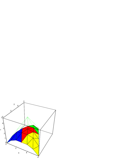
Figure 7: Subdivision, $1$ iteration

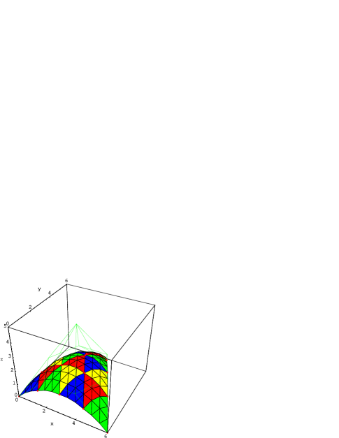
Figure 8: Subdivision, $2$ iterations

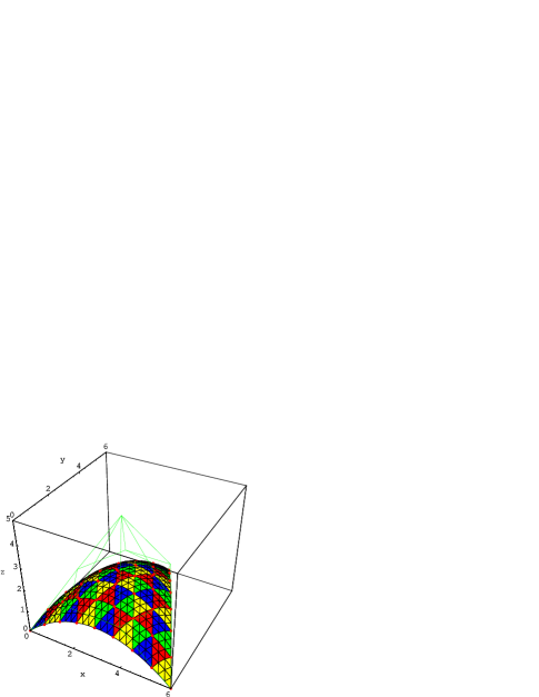
Figure 9: Subdivision, $3$ iterations

After only three subdivision steps, the triangulation approximates the surface patch very well.

As another example of the use of the above functions, we can display a portion of a well known surface known as the “monkey saddle”, defined by the equations

$$x=u,\quad y=v,\quad z=u^{3}-3uv^{2}.$$

Note that $z$ is the real part of the complex number $(u+iv)^{3}$. It is easily shown that the monkey saddle is specified by the following triangular control net monknet over the standard affine frame $\Delta rst$, where $r=(1,0,0)$, $s=(0,1,0)$, and $t=(0,0,1)$.

monknet = {{0, 0, 0}, {0, 1/3, 0}, {0, 2/3, 0}, {0, 1, 0},
          {1/3, 0, 0}, {1/3, 1/3, 0},  {1/3, 2/3, -1},
          {2/3, 0, 0}, {2/3, 1/3, 0},  {1, 0, 1}};

We actually display the patch over the rectangle $[-1,1]\times[-1,1]$. This can be done by splitting the square into two triangles, and computing control nets with respect to these triangles. This is easy to do, and it is explained for example in Gallier [9]. Subdividing both nets $3$ times, we get the following picture.

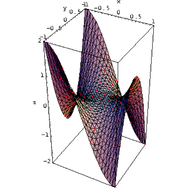
Figure 10: A monkey saddle, triangular subdivision

5 A Diamond-Shape Strategy For Subdivision

The strategy of the previous section was to split the affine frame $\Delta rts$ into four congruent subtriangles. We were able to do this using four calls to the de Casteljau algorithm and we showed that it is not possible to do it in fewer calls.

However, it is possible to split the affine frame into four subtriangles using only three calls to the de Casteljau algorithm. The method consists in splitting the triangle $\Delta rst$ into the four subtriangles $\Delta bat$, $\Delta bar$, $\Delta cas$, and $\Delta car$:

Figure 11: Diamond-style subdivision of an affine frame $\Delta rst$

This can be done by first computing the nets ${\cal N}art$ and ${\cal N}ars$, which can be done in one call to sdecas3 (dropping ${\cal N}ast$). Next, we split $\Delta art$ into the two triangles $\Delta bat$ and $\Delta bar$. For this, we need the barycentric coordinates of $b$ with respect to the triangle $\Delta art$, which turns out $(0,1/2,1/2)$. Using the function sdecas3, the nets ${\cal N}bat$, ${\cal N}brt$, and ${\cal N}bar$ are obtained, and we throw away ${\cal N}brt$. Finally, we split $\Delta ars$ into the two triangles $\Delta cas$ and $\Delta car$. For this, we need the barycentric coordinates of $c$ with respect to the triangle $\Delta ars$, which turns out $(0,1/2,1/2)$. Using the function sdecas3, the nets ${\cal N}cas$, ${\cal N}crs$, and ${\cal N}car$ are obtained, and we throw away ${\cal N}crs$.

An implementation of the method is given in Gallier [9].

The result of subdividing two of three times reveals some diamond-shape subdividion patterns. For example, after three iterations, the dome surface is subdivided as follows:

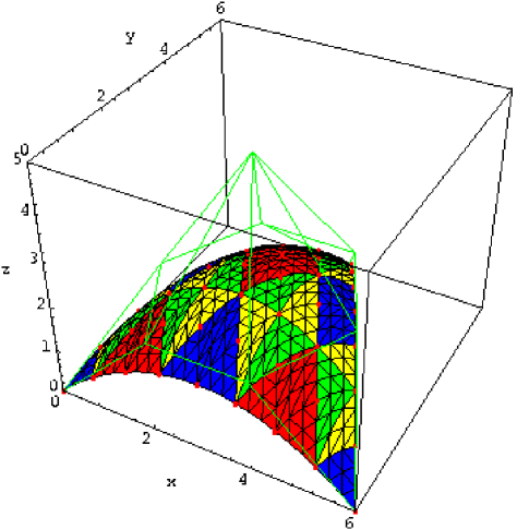
Figure 12: Diamond-style subdivision, $3$ iterations

6 A Spider-Web Strategy For Subdivision

Is is also possible to split the affine frame into six subtriangles using only four calls to the de Casteljau algorithm.

Figure 13: spider-web subdivision of an affine frame $\Delta rst$

The triangle $\Delta rst$ is subdivided into the triangles $\Delta bgt$, $\Delta bgr$, $\Delta agt$, $\Delta ags$, $\Delta cgs$, and $\Delta cgr$, as shown above, where $g$ is the center of gravity. This can be done by first computing the nets ${\cal N}grt$, ${\cal N}gst$, and ${\cal N}grs$, which can be done in one call to sdecas3. We split $\Delta grt$ into the two triangles $\Delta bgt$ and $\Delta bgr$ using sdecas3 (throwing away $\Delta brt$). We split $\Delta gst$ into the two triangles $\Delta agt$ and $\Delta ags$ using sdecas3 (throwing away $\Delta ast$). Finally, we split $\Delta grs$ into the two triangles $\Delta cgs$ and $\Delta cgs$ using sdecas3 (throwing away $\Delta crs$).

The result of subdividing recursively yields spider-web like patterns. For example, after three iterations, the dome surface is subdivided as follows:

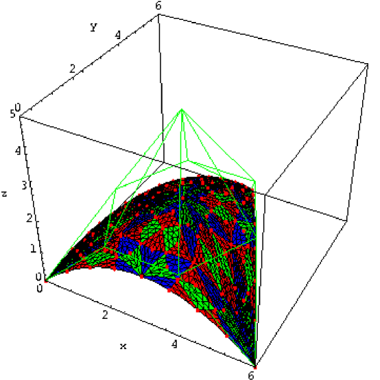
Figure 14: Spider-web style subdivision, $3$ iterations

7 Conclusion

We have presented various strategies for subdividing polynomial triangular surface patches. We gave an algorithm performing a regular subdivision in four calls to the standard de Casteljau algorithm, and we showed that this method for obtaining a regular subdivision is optimal. We gave another subdivision algorithm using only three calls to the de Casteljau algorithm. Instead of being regular, the subdivision pattern is diamond-like. Finally, we presented a “spider-web” pattern subdivision scheme producing six subtriangles in four calls to the de Casteljau algorithm. These methods immediately apply to rational surface patches (Gallier [10]).

An amusing effect is obtained from the regular subdivision scheme if we omit the central triangle $\Delta bac$. We obtain a “fractalized” representation of the surface patch, in the sense that a Sierpinski gasket pattern is laid onto the patch! It would be interesting to investigate other subdivision strategies and the patterns that they induce, especially if the triangles are colored in various recursive manners.

References

• [1] Marcel Berger. Géométrie 1. Nathan, 1990. English edition: Geometry 1, Universitext, Springer Verlag.
• [2] W. Boehm and G. Farin. Letter to the editor. Computer Aided Design, 15(5):260–261, 1983. Concerning subdivison of Bézier triangles.
• [3] W. Boehm, G. Farin, and J. Kahman. A survey of curve and surface methods in CAGD. Computer Aided Geometric Design, 1:1–60, 1984.
• [4] Wolfgang Böhm. Subdividing multivariate splines. Computer Aided Design, 15:345–352, 1983.
• [5] G. Farin. Triangular Bernstein-Bézier patches. Computer Aided Geometric Design, 3:83–127, 1986.
• [6] Gerald Farin. NURB Curves and Surfaces, from Projective Geometry to practical use. AK Peters, first edition, 1995.
• [7] Gerald Farin. Curves and Surfaces for CAGD. Academic Press, fourth edition, 1998.
• [8] D.J. Filip. Adapative subdivision algorithms for a set of Bézier triangles. Computer Aided Design, 18:74–78, 1986.
• [9] Jean H. Gallier. Curves and Surfaces In Geometric Modeling: Theory And Algorithms. Morgan Kaufmann, first edition, 1999.
• [10] Jean H. Gallier. Simple methods for drawing rational surfaces as four or six Bézier patches. Technical report, University of Pennsylvania, Levine Hall, 3330 Walnut, Philadelphia, PA 19104, 2006.
• [11] R. N. Goldman. Subdivision algorithms for Bézier triangles. Computer Aided Design, 15:159–166, 1983.
• [12] J. Hoschek and D. Lasser. Computer Aided Geometric Design. AK Peters, first edition, 1993.
• [13] Helmut Prautzsch. Unterteilungsalgorithmen für multivariate splines. PhD thesis, TU Braunschweig, Braunschweig, Germany, 1984. Dissertation.
• [14] Lyle Ramshaw. Blossoming: A connect-the-dots approach to splines. Technical report, Digital SRC, Palo Alto, CA 94301, 1987. Report No. 19.
• [15] J.-J. Risler. Mathematical Methods for CAD. Masson, first edition, 1992.
• [16] H.P. Seidel. A general subdivision theorem for Bézier triangles. In Tom Lyche and Larry Schumaker, editors, Mathematical Methods in Computer Aided Geometric Design, pages 573–581. Academic Press, Boston, Mass, 1989.