Belief Calculus

Abstract

In Dempster-Shafer belief theory, general beliefs are expressed as belief mass distribution functions over frames of discernment. In Subjective Logic beliefs are expressed as belief mass distribution functions over binary frames of discernment. Belief representations in Subjective Logic, which are called opinions, also contain a base rate parameter which express the a priori belief in the absence of evidence. Philosophically, beliefs are quantitative representations of evidence as perceived by humans or by other intelligent agents. The basic operators of classical probability calculus, such as addition and multiplication, can be applied to opinions, thereby making belief calculus practical. Through the equivalence between opinions and Beta probability density functions, this also provides a calculus for Beta probability density functions. This article explains the basic elements of belief calculus.

1 Introduction

Belief theory has its origin in a model for upper and lower probabilities proposed by Dempster in 1960. Shafer later proposed a model for expressing beliefs [7]. The main idea behind belief theory is to abandon the additivity principle of probability theory, i.e. that the sum of probabilities on all pairwise exclusive possibilities must add up to one. Instead belief theory gives observers the ability to assign so-called belief mass to any subset of the frame of discernment, i.e. non-exclusive possibilities including the whole frame itself. The main advantage of this approach is that ignorance, i.e. the lack of information, can be explicitly expressed e.g. by assigning belief mass to the whole frame. Shafer’s book [7] describes many aspects of belief theory, but the two main elements are 1) a flexible way of expressing beliefs, and 2) a method for combining beliefs, commonly known as Dempster’s Rule.

2 Representing Opinions

Belief representation in classic belief theory[7] is based on an exhaustive set of mutually exclusive atomic states which is called the frame of discernment $\Theta$. The power set $2^{\Theta}$ is the set of all sub-states of $\Theta$. A bba (basic belief assignment) is a belief distribution function $m_{\Theta}$ mapping $2^{\Theta}$ to $[0,1]$ such that

$$\sum_{x\subseteq{\Theta}}m_{\Theta}(x)=1\;,\;\mbox{ where }\;m_{\Theta}(\emptyset)=0\;.$$ (1)

The bba distributes a total belief mass of 1 amongst the subsets of $\Theta$ such that the belief mass for each subset is positive or zero. Each subset $x\subseteq\Theta$ such that $m_{\Theta}(x)>0$ is called a focal element of $m_{\Theta}$. In the case of total ignorance, $m_{\Theta}(\Theta)=1$, and $m_{\Theta}$ is called a vacuous bba. In case all focal elements are atoms (i.e. one-element subsets of $\Theta$) then we speak about Bayesian bba. A dogmatic bba is when $m_{\Theta}(\Theta)=0$ [8]. Let us note that, trivially, every Bayesian bba is dogmatic.

In addition, we also define the Dirichlet bba, and its cluster variant, as follows.

Definition 1 (Dirichlet bba)

A bba where the possible focal elements are $\Theta$ and/or singletons of $\Theta$, is called a Dirichlet belief distribution function.

Definition 2 (Cluster Dirichlet bba)

A bba where the only focal elements are $\Theta$ and/or mutually exclusive subsets of $\Theta$ (singletons or clusters of singletons), is called a cluster Dirichlet belief distribution function.

It can be noted that Bayesian bbas are a special case of Dirichlet bbas.

The Dempster-Shafer theory [7] defines a belief function $b(x)$. The probability transformation [1] projects a bba onto a probability expectation value denoted by $\mbox{E}(x)$. In addition, subjective logic [2] defines a disbelief function $d(x)$, an uncertainty function $u(x)$, and a base rate function $a(x)$, defined as follows:

$$b(x) =\sum_{\emptyset\neq y\subseteq x}m(y)\qquad \forall\;x\subseteq{\Theta}\;,$$ (2)

$$d(x) =\sum_{y\cap x=\emptyset}m(y)\qquad \forall\;x\subseteq{\Theta}\;,$$ (3)

$$u(x) =\sum_{\scriptsize\scriptsize\begin{array}[]{cc}{y}\cap{x}\neq\emptyset\\ {y}\not\subseteq{x}\end{array}}m(y)\qquad \forall\;x\subseteq{\Theta}\;,$$ (6)

$$a(x) ={{|x|}/{|\Theta}|}\qquad \forall\;x\subseteq{\Theta}\;,$$ (7)

$$\mathrm{E}(x) =\sum_{y\subseteq\Theta}m_{\Theta}(y)\frac{|x\cap y|}{|y|}\qquad \forall\;x\subseteq{\Theta}\;.$$ (8)

In case $|\Theta|>2$, coarsening is necessary in order to apply subjective logic operators. Choose $x\subseteq{\Theta}$, and let $\overline{x}$ be the complement of $x$ in $\Theta$, then $X=\{x,\overline{x}\}$ is a binary frame, and $x$ is called that target of the coarsening. The coarsened bba on $X$ can consist of the three belief masses $b_{x}=m_{X}(x)$, $d_{x}=m_{X}(\overline{x})$ and $u_{x}=m_{X}(X)$, called belief, disbelief and uncertainty respectively. Coarsened belief masses can be computed e.g. with simple or normal coarsening as defined in [2, 4], or with smooth coarsening defined next.

Definition 3 (Smooth Coarsening)

Let $\Theta$ be a frame of discernment and let $b(x)$, $d(x)$, $u(x)$ and $a(x)$ be the belief, disbelief, uncertainty and base rate functions of the target state ${x}\subseteq\Theta$, with probability expectation value $\mathrm{E}(x)$. Let $X=\{x,\overline{x}\}$ be the binary frame of discernment, where $\overline{x}$ is the complement of $x$ in $\Theta$. Smooth coarsening of $\Theta$ into $X$ produces the corresponding belief, disbelief, uncertainty and base rate functions $b_{x}$, $d_{x}$, $u_{x}$ and $a_{x}$ defined by:

$$\begin{array}[]{l}\mbox{For }\;\mathrm{E}(x)\leq b(x)+a(x)u(x)\;:\\ \hline\cr\\ \left\{\begin{array}[]{ll}b_{x}&=\frac{\mathrm{E}(x)b(x)}{b(x)+a(x)u(x)}\\ \\ d_{x}&=1-\frac{\mathrm{E}(x)(b(x)+u(x))}{b(x)+a(x)u(x)}\\ \\ u_{x}&=\frac{\mathrm{E}(x)u(x)}{b(x)+a(x)u(x)}\\ \\ a_{x}&=a(x)\;,\par\end{array}\right.\\ \\ \mbox{for }\;\mathrm{E}(x)>b(x)+a(x)u(x)\;:\\ \hline\cr\\ \left\{\begin{array}[]{ll}b_{x}&=1-\frac{(1-\mathrm{E}(x))(d(x)+u(x))}{1-b(x)-a(x)u(x)}\\ \\ d_{x}&=\frac{(1-\mathrm{E}(x))d(x)}{1-b(x)-a(x)u(x)}\\ \\ u_{x}&=\frac{(1-\mathrm{E}(x))u(x)}{1-b(x)-a(x)u(x)}\\ \\ a_{x}&=a(x)\;.\par\par\end{array}\right.\end{array}$$

In case the target element for the coarsening is a focal element of a (cluster) Dirichlet belief distribution function, $\mathrm{E}(x)=b(x)+a(x)u(x)$ holds, and the coarsening can be described as stable.

Definition 4 (Stable Coarsening)

Let $\Theta$ be a frame of discernment, and let $x\in\Theta$ be the target element for the coarsening. Let the belief distribution function be a Dirichlet (cluster or not) bba such that the target element is also a focal element. Then the stable coarsening of $\Theta$ into $X$ produces the belief, disbelief and uncertainty functions $b_{x}$, $d_{x}$ and $u_{x}$ defined by:

$$\begin{array}[]{lll}b_{x}=b(x)\;,&d_{x}=d(x)\;,&u_{x}=u(x)\;.\end{array}$$

It can be shown that $b_{x},d_{x},u_{x},a_{x}\in[0,1]$, and that Eq.(9) and Eq.(10) hold.

$$b_{x}+d_{x}+u_{x}=1\;.\;\;\;\;\;\;\mbox{(Additivity)}$$ (9)

$$\mathrm{E}(x)=b_{x}+a_{x}u_{x}\;.\;\;\;\;\;\mbox{(Expectation)}$$ (10)

It can be noticed that non-stable coarsening requires an adjustment of the belief, disbelief and uncertainty functions in general, and this can result in inconsistency when applying the consensus operator. The purpose of this paper is to present a method to rectify this problem. This will be explained in further detail in the sections below.

The ordered quadruple $\omega_{x}=(b_{x},\;d_{x},\;u_{x},\;a_{x})$, called the opinion about $x$, is equivalent to a bba on a binary frame of discernment $X$, with an additional base rate parameter $a_{x}$ which can carry information about the relative size of $x$ in $\Theta$.

The opinion space can be mapped into the interior of an equal-sided triangle, where the the relative distance towards the bottom right, bottom left and the top corners represent belief, disbelief and uncertainty functions respectively. For an arbitrary opinion $\omega_{x}=(b_{x},d_{x},u_{x},a_{x})$, the three parameters $b_{x}$, $d_{x}$ and $u_{x}$ determine the position of the opinion point in the triangle. The base line is the probability axis. The base rate value can be indicated as a point on the probability axis.

Fig.1 illustrates an example opinion about $x$ with the value $\omega_{x}=(0.7,\;0.1,\;0.2,\;0.5)$.

Figure 1: Opinion triangle with example opinion

The projector going through the opinion point, parallel to the line that joins the uncertainty corner and the base rate point, determines the probability expectation value $\mathrm{E}(x)=b_{x}+a_{x}u_{x}$.

Although an opinion has 4 parameters, it only has 3 degrees of freedom because the three components $b_{x}$, $d_{x}$ and $u_{x}$ are dependent through Eq.(9). As such they represent the traditional $\mbox{\it Bel}(x)$ (Belief) and $\mbox{\it Pl}(x)$ (Plausibility) pair of Shaferian belief theory through the correspondence $\mbox{\it Bel}(x)=b(x)$ and $\mbox{\it Pl}(x)=b(x)+u(x)$. The disbelief function $d(x)$ is the same as doubt of ${x}$ in Shafer’s book. However, ‘disbelief’ seems to be a better term because the case when it is certain that $x$ is false, is better described by ‘total disbelief’ than by ‘total doubt’.

The reason why a redundant parameter is kept in the opinion representation is that it allows for more compact expressions of opinion operators, see e.g. [2, 3, 4, 5, 6].

Various visualisations of opinions are possible to facilitate human interpretation. For this, see http://sky.fit.qut.edu.au/$\sim$josang/sl/demo/BV.html

3 Mapping Opinions to Beta PDFs

The beta-family of distributions is a continuous family of distribution functions indexed by the two parameters $\alpha$ and $\beta$. The beta distribution $\mbox{beta}(\alpha,\beta)$ can be expressed using the gamma function $\Gamma$ as:

$$\begin{array}[]{l}\mbox{beta}(\alpha,\beta)={{\Gamma(\alpha+\beta)}\over{\Gamma(\alpha)\Gamma(\beta)}}{P}^{\alpha-1}(1\!-\!{P})^{\beta-1}\;,\\ \mbox{ where }0\leq{P}\leq 1,\;\alpha>0,\;\beta>0\end{array}$$ (11)

with the restriction that the probability ${P}\neq 0$ if $\alpha<1$, and ${P}\neq 1$ if $\beta<1$. The probability expectation value of the beta distribution is given by:

$$\mathrm{E}(P)=\frac{\alpha}{\alpha+\beta}$$ (12)

, where $P$ is the random variable corresponding to the probability.

It can be observed that the beta PDF has two degrees of freedom whereas opinions have three degrees of freedom as explained in Sec.2. In order to define a bijective mapping between opinions and beta PDFs, we will augment the beta PDF expression with 1 additional parameter representing the prior, so that it also gets 3 degrees of freedom.

The $\alpha$ parameter represents the amount of evidence in favour a given outcome or statement, and the $\beta$ parameter represents the amount of evidence against the same outcome or statement. With a given state space, it is possible to express the a priori PDF using a base rate parameter in addition to the evidence parameters.

The beta PDF parameters with the prior base rate $a$ included can be defined as [2]:

$$\left\{\begin{array}[]{l}\alpha=r+2a,\\ \beta=s+2(1-a)\;,\end{array}\right.$$ (13)

where $a$ represents the a priori base rate, $r$ represents the amount of positive evidence, and $s$ represents the amount of negative evidence.

We define the augmented beta PDF, denoted $\varphi(r,s,a)$, with 3 parameters as:

$$\varphi(r,s,a)=\mbox{beta}(\alpha,\beta)\;,\mbox{given Eq.(\ref{eq:beta-correspondence})}.$$ (14)

This augmented beta distribution function distinguishes between the a priori base rate $a$, and the a posteriori observed evidence $(r,s)$.

The probability expectation value of the augmented Beta distribution is given by:

$$\mathrm{E}(P)=\frac{r+2a}{r+s+2}$$ (15)

, where $P$ is the random variable corresponding to the probability.

For example, when an urn contains unknown proportions of red and black balls, the likelihood of picking a red ball is not expected to be greater or less than that of picking a black ball, so the a priori probability of picking a red ball is $a=0.5$, and the a priori augmented beta distribution is $\varphi(0,0,\frac{1}{2})=\mbox{beta}(1,1)$ as illustrated in Fig.2.

Figure 2: A priori $\varphi(0,0,\frac{1}{2})$

Assume that an observer picks 8 balls, of which 7 turn out to be red and only one turns out to be black. The updated augmented beta distribution of the outcome of picking red balls is $\varphi(7,1,\frac{1}{2})=\mbox{beta}(8,2)$ which is illustrated in Fig.3.

Figure 3: Updated $\varphi(7,1,\frac{1}{2})$

The expression for augmented beta PDFs has 3 degrees of freedom and allows a bijective mapping to opinions [2], defined as:

$$\begin{array}[]{lll}\!\!\!\!\!\!\!\!\!\!\!\!\!\!\!\!\left\{\begin{array}[]{l}r=2b_{x}/u_{x}\\ s=2d_{x}/u_{x}\\ 1=b_{x}\!+\!d_{x}\!+\!u_{x}\\ a=a_{x}\;,\end{array}\right.\!\!\!\!\!\!\!&\Leftrightarrow\!\!\!\!\!&\left\{\begin{array}[]{l}b_{x}=r/(r\!+\!s\!+\!2)\\ d_{x}=s/(r\!+\!s\!+\!2)\\ u_{x}=2/(r\!+\!s\!+\!2)\\ a_{x}=a\;.\end{array}\right.\end{array}$$ (16)

It can be noted that under this correspondence, the example opinion of Fig.1 and the beta distribution of Fig.3 are equivalent.

4 Mapping Opinions to Basic Probability Vectors

Both the opinion and the augmented Beta representation have the inconvenience that they do not explicitly express the probability expectation value. Although simple to compute with either Eq.10 or Eq.15, it represent a barrier for quick and intuitive interpretation by humans. We therefore propose a representation in the form of a Basic Probability Vector with three degrees of freedom that explicitly expresses the probability expectation value.

Definition 5

Basic Probability Vector Let $\Theta$ be a frame of discernment where $x\subset\Theta$ , and let $e$ be the subjective probability expectation value of $x$ as seen by an observer $A$. Let $u$ be the uncertainty of $e$, equivalent to the uncertainty defined for opinions. Let $a$ be the base rate of $x$ in $\Theta$, equivalent of the base rate defined for opinions. The Basic Probability Vector, denoted by $\pi^{A}_{x}$, is defined as $\pi^{A}_{x}=(e,u,a)$

In this context, the probability $p$ is simple to interpret. In case $u=0$, then $e$ is a frequentist probability. In case $u=1$, then $e=a$, i.e. $a$ is the probability expectation value of an augmented Beta probability density function where $r=s=0$.

The equivalence between opinions and basic probability vectors is defined below. The uncertainty and base rate parameters are identical in both representations, and their mapping is therefore not needed.

$$\begin{array}[]{lll}\left\{\begin{array}[]{l}e=b+au\\ b+d+u=1\end{array}\right.&\Leftrightarrow&\left\{\begin{array}[]{ll}b=e-au\\ d=1-e-u(1-a)\end{array}\right.\end{array}$$ (17)

5 Addition and Subtraction of Opinions

Addition of beliefs corresponds to determining the probability of the disjunction of two mutually exclusive subsets in a frame of discernment, given the probabilities of the original addend subsets. This is illustrated in Fig.4 below.

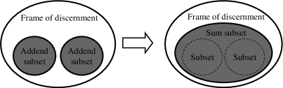
Figure 4: Addition principle

Subtraction of beliefs correspond to determining the probability of the difference of two subsets, given the probabilities of the original minuend and subtrahend subsets, where the subset of the minuend contains the subset of the subtrahend.

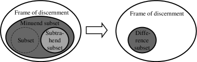
Figure 5: Subtraction principle

5.1 Addition of Opinions

The addition of opinions in subjective logic is a binary operator that takes opinions in a single frame of discernment about two mutually exclusive alternatives (i.e. two disjoint subsets of the frame of discernment), and outputs an opinion about the union of the subsets. Let the two sets be denoted by $x$ and $y$, so $x$ and $y$ are subsets of $\Theta$ such that $x\cap y=\emptyset$, then we are interested in the opinion about $x\cup y$, given opinions about $x$ and $y$. Since $x$ and $y$ are mutually exclusive, then it is to be expected that $b_{x}\leq d_{y}$ and $b_{y}\leq d_{x}$ as belief in either necessarily requires disbelief in the other. Since $x$ and $y$ are mutually exclusive, the belief in the union must be able to account for both the belief in $x$ and the belief in $y$, so that the first option that can be considered is $b_{x\cup y}=b_{x}+b_{y}$, so that $b_{x\cup y}$ has been partitioned exactly into the two possibilities. In order to calculate the atomicity of $x\cup y$, it is merely necessary to point out that

$$\begin{array}[]{ll}a(x\cup y)&=\frac{|x\cup y|}{|\Theta|}=\frac{|x|+|y|}{|\Theta|}=\frac{|x|}{|\Theta|}+\frac{|y|}{|\Theta|}\\ \\ &=a(x)+a(y),\end{array}$$

as $|x\cup y|=|x|+|y|$ since $x$ and $y$ are disjoint. Therefore the atomicity of $x\cup y$ is given by $a_{x\cup y}=a_{x}+a_{y}$. Similarly, the expectation value of $x\cup y$ must be given by

$$E(x\cup y)=E(x)+E(y),$$

since the probabilities of $x$ and $y$ are summed to calculate the probability of $x\cup y$ in probability calculus, and expectation value is linear on random variables (i.e. if $U$ and $V$ are random variables and $\mu$ and $\nu$ are real numbers, then $E[\mu U+\nu V]=\mu E[U]+\nu E[V]$). This gives us sufficient information to be able to calculate the opinion about $x\cup y$, with the result that

$$b_{x\cup y} =b_{x}+b_{y},$$ (18)

$$d_{x\cup y} =\frac{a_{x}(d_{x}-b_{y})+a_{y}(d_{y}-b_{x})}{a_{x}+a_{y}},$$ (19)

$$u_{x\cup y} =\frac{a_{x}u_{x}+a_{y}u_{y}}{a_{x}+a_{y}},$$ (20)

$$a_{x\cup y} =a_{x}+a_{y}.$$ (21)

By using the symbol “+” to denote the addition operator for opinions, we can write:

$$\omega_{x}+\omega_{y}=\omega_{x\cup y}\;.$$ (22)

Note that the uncertainty of $x\cup y$ is the weighted average of the uncertainties of $x$ and $y$, and the disbelief in $x\cup y$ is the weighted average of what is left in each case when the belief in one is subtracted from the disbelief in the other (when the amount of probability that neither is true is estimated), i.e. the disbelief in $x\cup y$ is the weighted average of the two estimates of the probability that the system is in neither the state $x$ nor the state $y$.

In the case where $u_{x}=u_{y}$ (i.e. $x$ and $y$ have the same uncertainty), then

$$b_{x\cup y} =b_{x}+b_{y},$$ (23)

$$d_{x\cup y} =d_{x}-b_{y}=d_{y}-b_{x},$$ (24)

$$u_{x\cup y} =u_{x}=u_{y},$$ (25)

$$a_{x\cup y} =a_{x}+a_{y},$$ (26)

so that the uncertainty in $x\cup y$ is equal to the common value of the uncertainty of $x$ and the uncertainty of $y$. The disbelief $d_{x\cup y}$ in $x\cup y$ is equal to the result when the belief in either is subtracted from the disbelief in the other. The fact that $d_{x\cup y}=d_{x}-b_{y}=d_{y}-b_{x}$ can be justified by the same sort of arguments that were used to justify $b_{x\cup y}=b_{x}+b_{y}$. Since the states $x$ and $y$ are mutually exclusive, then belief in $x$ necessitates disbelief in $y$, so that disbelief in $y$ can be partitioned into that part which corresponds to belief in $x$ (of magnitude $b_{x}$) and that part which corresponds to belief in neither $x$ nor $y$ (of magnitude $d_{y}-b_{x}$). Since the latter part of the disbelief in $y$ (of magnitude $d_{y}-b_{x}$) corresponds to belief in neither $x$ nor $y$, then it corresponds to disbelief in $x\cup y$, and so it is reasonable that $d_{x\cup y}=d_{y}-b_{x}$.

Various considerations make it natural that disjoint states in the frame of discernment should have the same uncertainty (and in fact, by the same considerations, all states in the frame of discernment should have the same uncertainty), especially if the a priori opinions are being formed, so that the uncertainty is equal to 1 to reflect the complete ignorance about the probabilities, and through updating due to evidence, where the uncertainty is dependent only on the amount of evidence that has been gathered. But this does not mean that the formulae given in Equations 18-21 should be disregarded. As noted in the Introduction, there are various operators which can be applied to opinions, and if the results of two such calculations result in opinions about two disjoint states in the same frame of discernment, the likelihood is that the opinions about the two states have unequal uncertainties, and the formulae that have to be used to calculate the sum of the opinions are Equations 18-21, rather than the simpler formulae in Equations 23-26. This is certainly the case, for example, when $x_{1}$ and $x_{2}$ are states in one frame of discernment, and $y_{1}$ and $y_{2}$ are states in another frame of discernment, and either $x_{1}$ and $x_{2}$ are disjoint states, or $y_{1}$ and $y_{2}$ are disjoint states. If the simple products [4] of opinions ($x_{1}\land y_{1}$ and $x_{2}\land y_{2}$) are determined, then they will almost certainly not have the same uncertainty. Similarly, if the normal products [4] are determined, then they will almost certainly not have the same uncertainty.

5.2 Subtraction of Opinions

The inverse operation to addition is subtraction. Since addition of opinions yields the opinion about $x\cup y$ from the opinions about disjoint subsets of the frame of discernment, then the difference between the opinions about $x$ and $y$ (i.e. the opinion about $x\backslash y$) can only be defined if $y\subseteq x$ where $x$ and $y$ are being treated as subsets of $\Theta$, the frame of discernment, i.e. the system must be in the state $x$ whenever it is in the state $y$. The opinion about $x\backslash y$ is the opinion about that state which consists exactly of the atomic states of $x$ which are not also atomic states of $y$, i.e. the opinion about the state in which the system is in the state $x$ but not in the state $y$. Since $y\subseteq x$, then belief in $y$ requires belief in $x$, and disbelief in $x$ requires disbelief in $y$, so that it is reasonable to require that $b_{x}\geq b_{y}$ and $d_{x}\leq d_{y}$. Since $y\subseteq x$, then $|y|\leq|x|$, so that $a(y)\leq a(x)$, and so $a_{y}\leq a_{x}$. The opinion about $x\backslash y$ is given by

$$b_{x\backslash y} =b_{x}-b_{y},$$ (27)

$$d_{x\backslash y} =\frac{a_{x}(d_{x}+b_{y})-a_{y}(1+b_{y}-b_{x}-u_{y})}{a_{x}-a_{y}},$$ (28)

$$u_{x\backslash y} =\frac{a_{x}u_{x}-a_{y}u_{y}}{a_{x}-a_{y}},$$ (29)

$$a_{x\backslash y} =a_{x}-a_{y}.$$ (30)

Since $u_{x\backslash y}$ should be nonnegative, then this requires that $a_{y}u_{y}\leq a_{x}u_{x}$, and since $d_{x\backslash y}$ should be nonnegative, then this requires that $a_{x}(d_{x}+b_{y})\geq a_{y}(1+b_{y}-b_{x}-u_{y})$.

By using the symbol “-” to denote the subtraction operator for opinions, we can write:

$$\omega_{x}-\omega_{y}=\omega_{x\backslash y}\;.$$ (31)

In the case where $u_{x}=u_{y}$ (i.e. $x$ and $y$ have the same uncertainty), then

$$b_{x\backslash y} =b_{x}-b_{y},$$ (32)

$$d_{x\backslash y} =d_{x}+b_{y},$$ (33)

$$u_{x\backslash y} =u_{x}=u_{y},$$ (34)

$$a_{x\backslash y} =a_{x}-a_{y},$$ (35)

so that the uncertainty in $x\backslash y$ is equal to the common value of the uncertainty of $x$ and the uncertainty of $y$. The belief $b_{x\backslash y}$ in $x\backslash y$ is all the belief in $x$ (of magnitude $b_{x}$) except for that part which is also belief in $y$ (of magnitude $b_{y}$), so that $b_{x\backslash y}=b_{x}-b_{y}$. The disbelief $d_{x\backslash y}$ in $x\backslash y$ is equal to the sum of the disbelief in $x$ and the belief in $y$. The fact that $d_{x\backslash y}=d_{x}+b_{y}$ can be justified as follows. Since the state $y$ necessitates the state $x$ (i.e the system must be in the state $x$ if it is in the state $y$), then disbelief in $x\backslash y$ falls into two categories: disbelief in $x$ (of magnitude $d_{x}$) and belief in $y$ (of magnitude $b_{y}$), with the result that the disbelief in $x\backslash y$ should be $d_{x}+b_{y}$.

5.3 Negation

The negation of an opinion about proposition $x$ represents the opinion about $x$ being false. This corresponds to ‘NOT’ in binary logic.

Definition 6 (Negation)

Let ${\omega}_{{x}}=(b_{x},d_{x},{u}_{x},{a}_{x})$ be an opinion about the proposition ${x}$. Then ${\omega}_{\lnot{x}}=(b_{\lnot{x}},d_{\lnot{x}},{u}_{\lnot{x}},{a}_{\lnot{x}})$ is the negation of ${\omega}_{x}$ where:

$$\begin{array}[]{l}b_{\lnot{x}}=d_{x}\\ d_{\lnot{x}}=b_{x}\\ u_{\lnot{x}}={u}_{x}\\ a_{\lnot{x}}=1-{a}_{x}\;.\end{array}$$

By using the symbol ‘$\;\lnot$’ to designate this operator, we define $\lnot{\omega}_{x}\equiv{\omega}_{\lnot x}$.

Negation can be applied to expressions containing propositional conjunction and disjunction, and it can be shown that De Morgans’s laws are valid.

6 Products of Binary Frames of Discernment

Multiplication and comultiplication in subjective logic are binary operators that take opinions about two elements from distinct binary frames of discernment as input parameters. The product and coproduct opinions relate to subsets of the Cartesian product of the two binary frames of discernment. The Cartesian product of the two binary frames of discernment $X=\{x,\overline{x}\}$ and $Y=\{y,\overline{y}\}$ produces the quaternary set $X\times Y=\{(x,y),\;(x,\overline{y}),\;(\overline{x},y),\;(\overline{x},\overline{y})\}$ which is illustrated in Fig.6 below.

Figure 6: Cartesian product of two binary frames of discernment

Let $\omega_{x}$ and $\omega_{y}$ be opinions about $x$ and $y$ respectively held by the same observer. Then the product opinion $\omega_{x\land y}$ is the observer’s opinion about the conjunction $x\land y=\{(x,y)\}$ that is represented by the area inside the dotted line in Fig.6. The coproduct opinion $\omega_{x\lor y}$ is the opinion about the disjunction $x\lor y=\{(x,y),\;(x,\overline{y}),\;(\overline{x},y)\}$ that is represented by the area inside the dashed line in Fig.6. Obviously $X\times Y$ is not binary, and coarsening is required in order to determine the product and coproduct opinions. The reduced powerset $2^{X\times Y}-\{\emptyset\}$ contains $2^{|X\times Y|}-1=15$ elements. A short notation for the elements of $2^{X\times Y}$ is used below so that for example $\{(x,y),\;(x,\overline{y})\}=\{x\}\times Y$. The bba on $X\times Y$ as a function of the opinions on $x$ and $y$ is defined by:

$$\begin{array}[]{lll}\begin{array}[]{r}m(\{(x,y)\})=b_{x}b_{y}\;,\\ m(\{(x,\overline{y})\})=b_{x}d_{y}\;,\\ m(\{x\}\times Y)=b_{x}u_{y}\;,\\ \end{array}&\begin{array}[]{r}m(\{(\overline{x},y)\})=d_{x}b_{y}\;,\\ m(\{(\overline{x},\overline{y})\})=d_{x}d_{y}\;,\\ m(\{\overline{x}\}\times Y)=d_{x}u_{y}\;,\\ \end{array}&\begin{array}[]{r}m(X\times\{y\})=u_{x}b_{y}\;,\\ m(X\times\{\overline{y}\})=u_{x}d_{y}\;,\\ m(X\times Y)=u_{x}u_{y}\;.\end{array}\end{array}$$ (36)

It can be shown that the sum of the above belief masses always equals 1. The product does not produce any belief mass on the following elements:

$$\begin{array}[]{lll}\begin{array}[]{c}\{(x,y),\;(\overline{x},\overline{y})\}\;,\\ \{(x,\overline{y}),\;(\overline{x},y)\}\;,\end{array}\;\;\;\begin{array}[]{c}(X\times\{y\})\cup\{(x,\overline{y})\}\;,\\ (X\times\{y\})\cup\{(\overline{x},\overline{y})\}\;,\end{array}\;\;\;\begin{array}[]{c}(X\times\{\overline{y}\})\cup\{(x,y)\}\;,\\ (X\times\{\overline{y}\})\cup\{(\overline{x},y)\})\;.\end{array}\end{array}$$ (37)

The belief functions in for example $x\land y$ and $x\lor y$ can now be determined so that:

$$\begin{array}[]{ll}b(x\land y)=&m(\{(x,y)\}),\\ b(x\lor y)=&m(\{(x,y)\})+m(\{(x,\overline{y})\})+m(\{(\overline{x},y)\})\;+\\ &m(\{x\}\times Y)+m(X\times\{y\})\;.\end{array}$$ (38)

The normal base rate functions for $x\land y$ and $x\lor y$ can be determined by working in the respective “primitive” frames of discernment, $\Theta_{X}$ and $\Theta_{Y}$ which underlie the definitions of the sets $x$ and $y$, respectively. A sample yields a value of $(x,y)$ in the frame of discernment $X\times Y$ exactly when the sample yields an atom $\theta_{X}\in x$ in the frame of discernment $\Theta_{X}$ and an atom $\theta_{Y}\in y$ in the frame of discernment $\Theta_{Y}$. In other words, a sample yields a value of $(x,y)$ in the frame of discernment $X\times Y$ exactly when the sample yields an atom $(\theta_{X},\theta_{Y})\in x\times y$ in the frame of discernment $\Theta_{X}\times\Theta_{Y}$, so that $(x,y)\in X\times Y$ corresponds to $x\times y\subseteq\Theta_{X}\times\Theta_{Y}$ in a natural manner. Similarly, $(x,\overline{y})$ corresponds to $x\times\overline{y}$, $(\overline{x},y)$ corresponds to $\overline{x}\times y$, and $(\overline{x},\overline{y})$ corresponds to $\overline{x}\times\overline{y}$. The normal base rate function for $x\land y$ is equal to:

$$a(x\land y)={{|x\times y|}\over{|\Theta_{X}\times\Theta_{Y}|}}={{|x|\;|y|}\over{|\Theta_{X}|\;|\Theta_{Y}|}}={{|x|}\over{|\Theta_{X}|}}\;{{|y|}\over{|\Theta_{Y}|}}=a(x)a(y),$$ (39)

Similarly, the normal base rate of $x\lor y$ is equal to

$$a(x\lor y) = \frac{|(x\times y)\cup(x\times\overline{y})\cup(\overline{x}\times y)|}{|\Theta_{X}\times\Theta_{Y}|}=\frac{|x\times y|+|x\times\overline{y}|+|\overline{x}\times y|}{|\Theta_{X}\times\Theta_{Y}|}$$

$$= \frac{|x|\;|y|+|x|\;|\overline{y}|+|\overline{x}|\;|y|}{|\Theta_{X}|\;|\Theta_{Y}|}=a(x)a(y)+a(x)a(\overline{y})+a(\overline{x})a(y)$$

$$= a(x)+a(y)-a(x)a(y).$$

By applying simple or normal coarsening to the product frame of discernment and bba, the normal product and coproduct opinions emerge. A coarsening that focuses on $x\land y$ produces the product, and a coarsening that focuses on $x\lor y$ produces the coproduct. A Bayesian coarsening (i.e. when simple and normal coarsening are equivalent) is only possible in exceptional cases because some terms of Eq.(36) other than $m(X\times Y)$ will in general contribute to uncertainty about $x\land y$ in the case of multiplication, and to uncertainty about $x\lor y$ in the case of comultiplication. Specifically, Bayesian coarsening requires $m(X\times\{y\})=m(\{x\}\times Y)=0$ in case of multiplication, and $m(X\times\{\overline{y}\})=m(\{\overline{x}\}\times Y)=0$ in case of comultiplication. Non-Bayesian coarsenings will cause the product and coproduct of opinions to deviate from the analytically correct product and coproduct. However, the magnitude of this deviation is always small, as shown in [4].

The symbols “$\cdot$” and “$\sqcup$” will be used to denote multiplication and comultiplication of opinions respectively so that we can write:

$$\omega_{x\land y} \triangleq\omega_{x}\cdot\omega_{y}$$ (40)

$$\omega_{x\lor y} \triangleq\omega_{x}\sqcup\omega_{y}$$ (41)

The product of the opinions about $x$ and $y$ is thus the opinion about the conjunction of $x$ and $y$. Similarly, the coproduct of the opinions about $x$ and $y$ is the opinion about the disjunction of $x$ and $y$. The exact expressions for product and coproduct are given in Sec.6.1.

Readers might have noticed that Eq.(36) can appear to be a direct application of the non-normalised version of Dempster’s rule (i.e. the conjunctive rule of combination) [7] which is a method of belief fusion. However the difference is that Dempster’s rule applies to the beliefs of two different and independent observers faced with the same frame of discernment, whereas the Cartesian product of Eq.(36) applies to the beliefs of the same observer faced with two different and independent frames of discernment. Let $\omega^{A}_{x}$ and $\omega^{B}_{x}$ represent the opinions of two observers $A$ and $B$ about the same proposition $x$, and let $\omega^{A,B}_{x}$ represent the fusion of $A$ and $B$’s opinions. Let further $\omega^{A}_{x}$ and $\omega^{A}_{y}$ represent observer $A$’s opinions about the propositions $x$ and $y$, and let $\omega^{A}_{x\land y}$ represent the product of those opinions. Fig.7 below illustrates the difference between belief fusion and belief product.

  

(a) Belief fusion.

(b) Belief product.

Figure 7: Conceptual difference between belief fusion and belief product.

The Cartesian product as described here thus has no relationship to Dempster’s rule and belief fusion other than the apparent similarity between Eq.(36) and Dempster’s rule.

6.1 Normal Multiplication and Comultiplication

Normal multiplication and comultiplication of opinions about independent propositions $x$ and $y$ are based on normal coarsening defined in [4]. It is also straightforward to define multiplication and comultiplication based on smooth coarsening, as defined here.

By the arguments within Section 6 for justifying the base rates, we can set $a_{x\land y}=a_{x}a_{y}$ and $a_{x\lor y}=a_{x}+a_{y}-a_{x}a_{y}$. This is in contrast to the case of “simple” conjunction and “simple” disjunction as discussed above, where atomicities of both the conjunction and the disjunction are dependent on the beliefs, disbeliefs and uncertainties of $x$ and $y$. Given opinions about independent propositions, $x$ and $y$, then under normal coarsening of the bba for the Cartesian product of the binary frames of discernment, the normal opinion for the conjunction, $x\land y$, is given by

$$b_{x\land y} = \frac{(b_{x}+a_{x}u_{x})(b_{y}+a_{y}u_{y})-(1-d_{x})(1-d_{y})a_{x}a_{y}}{1-a_{x}a_{y}}$$

$$= b_{x}b_{y}+\frac{(1-a_{x})a_{y}b_{x}u_{y}+a_{x}(1-a_{y})u_{x}b_{y}}{1-a_{x}a_{y}},$$

$$d_{x\land y} = d_{x}+d_{y}-d_{x}d_{y},$$

$$u_{x\land y} = \frac{(1-d_{x})(1-d_{y})-(b_{x}+a_{x}u_{x})(b_{y}+a_{y}u_{y})}{1-a_{x}a_{y}}$$

$$= u_{x}u_{y}+\frac{(1-a_{y})b_{x}u_{y}+(1-a_{x})u_{x}b_{y}}{1-a_{x}a_{y}},$$

$$a_{x\land y} = a_{x}a_{y}.$$

A numerical example of the normal multiplication operator is visualised in Fig.8 below. Note that in this case, the base rate $a_{x\land y}$ is equal to the real relative cardinality of $x\land y$ in $X\times Y$.

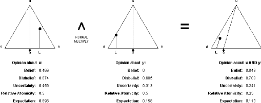
Figure 8: Visualisation of numerical example of the normal multiplication operator

The formulae for the opinion about $x\land y$ are well formed unless $a_{x}=1$ and $a_{y}=1$, in which case the opinions $\omega_{x}$ and $\omega_{y}$ can be regarded as limiting values, and the product is determined by the relative rates of approach of $a_{x}$ and $a_{y}$ to $1$. Specifically, if $\eta$ is the limit of $\frac{1-a_{x}}{1-a_{y}}$, then

$$b_{x\land y} = b_{x}b_{y}+\frac{\eta b_{x}u_{y}+u_{x}b_{y}}{\eta+1},$$

$$d_{x\land y} = d_{x}+d_{y}-d_{x}d_{y},$$

$$u_{x\land y} = u_{x}u_{y}+\frac{b_{x}u_{y}+\eta u_{x}b_{y}}{\eta+1},$$

$$a_{x\land y} = 1.$$

Under normal coarsening of the bba for the Cartesian product of the binary frames of discernment, the normal opinion for the disjunction, $x\lor y$, is given by

$$b_{x\lor y} = b_{x}+b_{y}-b_{x}b_{y},$$

$$d_{x\lor y} = \frac{(1-(b_{x}+a_{x}u_{x}))(1-(b_{y}+a_{y}u_{y}))-(1-b_{x})(1-b_{y})(1-a_{x})(1-a_{y})}{a_{x}+a_{y}-a_{x}a_{y}}$$

$$= \frac{(d_{x}+(1-a_{x})u_{x})(d_{y}+(1-a_{y})u_{y})-(1-b_{x})(1-b_{y})(1-a_{x})(1-a_{y})}{a_{x}+a_{y}-a_{x}a_{y}}$$

$$= d_{x}d_{y}+\frac{a_{x}(1-a_{y})d_{x}u_{y}+(1-a_{x})a_{y}u_{x}d_{y}}{a_{x}+a_{y}-a_{x}a_{y}},$$

$$u_{x\lor y} = \frac{(1-b_{x})(1-b_{y})-(1-(b_{x}+a_{x}u_{x}))(1-(b_{y}+a_{y}u_{y}))}{a_{x}+a_{y}-a_{x}a_{y}}$$

$$= \frac{(1-b_{x})(1-b_{y})-(d_{x}+(1-a_{x})u_{x})(d_{y}+(1-a_{y})u_{y})}{a_{x}+a_{y}-a_{x}a_{y}}$$

$$= u_{x}u_{y}+\frac{a_{y}d_{x}u_{y}+a_{x}u_{x}d_{y}}{a_{x}+a_{y}-a_{x}a_{y}},$$

$$a_{x\lor y} = a_{x}+a_{y}-a_{x}a_{y}.$$

A numerical example of the normal comultiplication operator is visualised in Fig.9 below. Note that in this case, the base rate $a_{x\lor y}$ is equal to the real relative cardinality of $x\lor y$ in $X\times Y$.

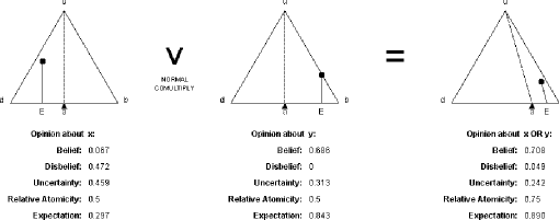
Figure 9: Visualisation of numerical example of the normal comultiplication operator

The formulae for the opinion about $x\lor y$ are well formed unless $a_{x}=0$ and $a_{y}=0$. In the case that $a_{x}=a_{y}=0$, the opinions $\omega_{x}$ and $\omega_{y}$ can be regarded as limiting values, and the product is determined by the relative rates of approach of $a_{x}$ and $a_{y}$ to $0$. Specifically, if $\zeta$ is the limit of $\frac{a_{x}}{a_{y}}$, then

$$b_{x\lor y} = b_{x}+b_{y}-b_{x}b_{y},$$

$$d_{x\lor y} = d_{x}d_{y}+\frac{\zeta d_{x}u_{y}+u_{x}d_{y}}{\zeta+1},$$

$$u_{x\lor y} = u_{x}u_{y}+\frac{d_{x}u_{y}+\zeta u_{x}d_{y}}{\zeta+1},$$

$$a_{x\lor y} = 0.$$

This is a self-dual system under $b\leftrightarrow d$, $u\leftrightarrow u$, $a\leftrightarrow 1-a$, and $\land\leftrightarrow\lor$, that is, for example, the expressions for $b_{x\land y}$ and $d_{x\lor y}$ are dual to each other, and one determines the other by the correspondence, and similarly for the other expressions. This is equivalent to the observation that the opinions satisfy de Morgan’s Laws, i.e. $\omega_{x\land y}=\omega_{\overline{\overline{x}\lor\overline{y}}}$ and $\omega_{x\lor y}=\omega_{\overline{\overline{x}\land\overline{y}}}$.

However it should be noted that multiplication and comultiplication are not distributive over each other, i.e. for example that:

$$\omega_{x\land(y\lor z)}\neq\omega_{(x\land y)\lor(x\land z)}$$ (42)

This is to be expected because if $x$, $y$ and $z$ are independent, then $x\land y$ and $x\land z$ are not generally independent in probability calculus. In fact the corresponding result only holds for binary logic.

6.2 Normal Division and Codivision

The inverse operation to multiplication is division. The quotient of opinions about propositions $x$ and $y$ represents the opinion about a proposition $z$ which is independent of $y$ such that $\omega_{x}=\omega_{y\land z}$. This requires that $a_{x}\leq a_{y}$, $d_{x}\geq d_{y}$, and

$$b_{x} \geq \frac{a_{x}(1-a_{y})(1-d_{x})b_{y}}{(1-a_{x})a_{y}(1-d_{y})},$$

$$u_{x} \geq \frac{(1-a_{y})(1-d_{x})u_{y}}{(1-a_{x})(1-d_{y})}.$$

The opinion $(b_{x\overline{\land}y},d_{x\overline{\land}y},u_{x\overline{\land}y},a_{x\overline{\land}y})$, which is the quotient of the opinion about $x$ and the opinion about $y$, is given by

$$b_{x\overline{\land}y} = \frac{a_{y}(b_{x}+a_{x}u_{x})}{(a_{y}-a_{x})(b_{y}+a_{y}u_{y})}-\frac{a_{x}(1-d_{x})}{(a_{y}-a_{x})(1-d_{y})},$$

$$d_{x\overline{\land}y} = \frac{d_{x}-d_{y}}{1-d_{y}},$$

$$u_{x\overline{\land}y} = \frac{a_{y}(1-d_{x})}{(a_{y}-a_{x})(1-d_{y})}-\frac{a_{y}(b_{x}+a_{x}u_{x})}{(a_{y}-a_{x})(b_{y}+a_{y}u_{y})},$$

$$a_{x\overline{\land}y} = \frac{a_{x}}{a_{y}},$$

if $a_{x}<a_{y}$. If $0<a_{x}=a_{y}$, then the conditions required so that the opinion about $x$ can be divided by the opinion about $y$ are

$$b_{x} = \frac{(1-d_{x})b_{y}}{1-d_{y}},$$

$$u_{x} = \frac{(1-d_{x})u_{y}}{1-d_{y}},$$

and in this case,

$$d_{x\overline{\land}y} = \frac{d_{x}-d_{y}}{1-d_{y}},$$

$$a_{x\overline{\land}y} = 1.$$

The only information available about $b_{x\overline{\land}y}$ and $u_{x\overline{\land}y}$ is that

$$b_{x\overline{\land}y}+u_{x\overline{\land}y}=\frac{1-d_{x}}{1-d_{y}}.$$

On the other hand, $b_{x\overline{\land}y}$ and $u_{x\overline{\land}y}$ can be determined if the opinion about $x$ is considered as the limiting value of other opinions which can be divided by the opinion about $y$. The limiting value of the quotient of the opinions is determined by the relative rates of approach of $a_{x}$, $b_{x}$ and $u_{x}$ to their limits. Specifically, if $\gamma$ is the limit of

$$\frac{a_{y}(1-a_{y})}{(a_{y}-a_{x})(b_{y}+a_{y}u_{y})}\left(\frac{(1-d_{y})b_{x}}{1-d_{x}}-b_{y}\right)+\frac{b_{y}}{b_{y}+a_{y}u_{y}},$$

then $0\leq\gamma\leq 1$, and the limiting values of $b_{x\overline{\land}y}$ and $u_{x\overline{\land}y}$ are

$$b_{x\overline{\land}y} = \frac{\gamma(1-d_{x})}{1-d_{y}},$$

$$u_{x\overline{\land}y} = \frac{(1-\gamma)(1-d_{x})}{1-d_{y}}.$$

The inverse operation to comultiplication is codivision. The co-quotient of opinions about propositions $x$ and $y$ represents the opinion about a proposition $z$ which is independent of $y$ such that $\omega_{x}=\omega_{y\lor z}$. This requires that $a_{x}\geq a_{y}$, $b_{x}\geq b_{y}$, and

$$d_{x} \geq \frac{(1-a_{x})a_{y}(1-b_{x})d_{y}}{a_{x}(1-a_{y})(1-b_{y})},$$

$$u_{x} \geq \frac{a_{y}(1-b_{x})u_{y}}{a_{x}(1-b_{y})}.$$

The opinion $(b_{x\overline{\lor}y},d_{x\overline{\lor}y},u_{x\overline{\lor}y},a_{x\overline{\lor}y})$, which is the co-quotient of the opinion about $x$ and the opinion about $y$, is given by

$$b_{x\overline{\lor}y} = \frac{b_{x}-b_{y}}{1-b_{y}},$$

$$d_{x\overline{\lor}y} = \frac{(1-a_{y})(1-(b_{x}+a_{x}u_{x}))}{(a_{x}-a_{y})(1-(b_{y}+a_{y}u_{y}))}-\frac{(1-a_{x})(1-b_{x})}{(a_{x}-a_{y})(1-b_{y})}$$

$$= \frac{(1-a_{y})(d_{x}+(1-a_{x})u_{x})}{(a_{x}-a_{y})(d_{y}+(1-a_{y})u_{y})}-\frac{(1-a_{x})(1-b_{x})}{(a_{x}-a_{y})(1-b_{y})},$$

$$u_{x\overline{\lor}y} = \frac{(1-a_{y})(1-b_{x})}{(a_{x}-a_{y})(1-b_{y})}-\frac{(1-a_{y})(1-(b_{x}+a_{x}u_{x}))}{(a_{x}-a_{y})(1-(b_{y}+a_{y}u_{y}))}$$

$$= \frac{(1-a_{y})(1-b_{x})}{(a_{x}-a_{y})(1-b_{y})}-\frac{(1-a_{y})(d_{x}+(1-a_{x})u_{x})}{(a_{x}-a_{y})(d_{y}+(1-a_{y})u_{y})},$$

$$a_{x\overline{\lor}y} = \frac{a_{x}-a_{y}}{1-a_{y}},$$

if $a_{x}>a_{y}$. If $a_{x}=a_{y}<1$, then the conditions required so that the opinion about $x$ can be codivided by the opinion about $y$ are

$$d_{x} = \frac{(1-b_{x})d_{y}}{1-b_{y}},$$

$$u_{x} = \frac{(1-b_{x})u_{y}}{1-b_{y}},$$

and in this case,

$$b_{x\overline{\lor}y} = \frac{b_{x}-b_{y}}{1-b_{y}},$$

$$a_{x\overline{\lor}y} = 0.$$

The only information available about $d_{x\overline{\lor}y}$ and $u_{x\overline{\lor}y}$ is that

$$d_{x\overline{\lor}y}+u_{x\overline{\lor}y}=\frac{1-b_{x}}{1-b_{y}}.$$

On the other hand, $d_{x\overline{\lor}y}$ and $u_{x\overline{\lor}y}$ can be determined if the opinion about $x$ is considered as the limiting value of other opinions which can be codivided by the opinion about $y$. The limiting value of the co-quotient of the opinions is determined by the relative rates of approach of $a_{x}$, $d_{x}$ and $u_{x}$ to their limits. Specifically, if $\delta$ is the limit of

$$\frac{a_{y}(1-a_{y})}{(a_{x}-a_{y})(d_{y}+(1-a_{y})u_{y})}\left(\frac{(1-b_{y})d_{x}}{1-b_{x}}-d_{y}\right)+\frac{d_{y}}{d_{y}+(1-a_{y})u_{y}},$$

then $0\leq\delta\leq 1$, and the limiting values of $d_{x\overline{\lor}y}$ and $u_{x\overline{\lor}y}$ are

$$d_{x\overline{\lor}y} = \frac{\delta(1-b_{x})}{1-b_{y}},$$

$$u_{x\overline{\lor}y} = \frac{(1-\delta)(1-b_{x})}{1-b_{y}}.$$

Given the opinion about $x$ and the atomicity of $y$, it is possible to use the triangular representation of the opinion space from Fig.1 to describe geometrically the range of opinions about $x\land y$ and $x\lor y$.

In the case of $x\land y$, take the projector for $\omega_{x}$, and take the intersections of the projector with the line of zero uncertainty and the line of zero belief ($A$ and $B$, respectively). The intersection, $A$, with the line of zero uncertainty determines the probability expectation value of $\omega_{x}$. Take the point, $C$, on the line of zero uncertainty whose distance from the disbelief vertex is $a_{y}$ times the distance between the disbelief vertex and $A$. Take the line $BC$ and the line through $A$ parallel to $BC$. Let $D$ and $E$ be the intersections of these lines with the line of constant disbelief through $\omega_{x}$, so that the disbelief is equal to $d_{x}$. Then $\omega_{x\land y}$ falls in the closed triangle determined by $D$, $E$ and the disbelief vertex, and the atomicity of $x\land y$ is given by $a_{x\land y}=a_{x}a_{y}$.

In Fig. 10, this is demonstrated with an example where $\omega_{x}=(0.3,0.3,0.4,0.6)$ and $a_{y}=0.4$. The opinion $\omega_{x}$ has been marked with a small black circle (on the side of the shaded triangle opposite the disbelief vertex). The intersections $A$ and $B$ of the projector of $x$ with the line of zero uncertainty and the line of zero belief, respectively, have been marked. The point $C$ has been placed on the probability axis so that its distance from the disbelief vertex is 0.4 times the distance between $A$ and the disbelief vertex (since $a_{y}=0.4$). The line $BC$, whose direction corresponds to an atomicity of 0.24 (i.e. the atomicity of $x\land y$), has also been drawn in the triangle, and its intersection with the line of constant disbelief through $\omega_{x}$ (with disbelief equal to 0.3) has been marked with a white circle. This is the point $D$, although not marked as such in the figure. The line through $A$ parallel to $BC$ has also been drawn in the triangle, and its intersection with the line of constant disbelief through $\omega_{x}$ (the point $E$, although also not marked as such) has also been marked with a white circle. The triangle with vertices $D$, $E$ and the disbelief vertex has been shaded, and the normal product $\omega_{x\land y}$ of the opinions must fall within the shaded triangle or on its boundary. In other words, the closure of the shaded triangle is the range of all possible values for the opinion $\omega_{x\land y}$.

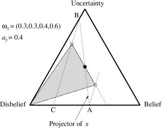
Figure 10: Range of possible opinions for normal product

In the case of $x\lor y$, take the projector for $\omega_{x}$, and take the intersections of this line with the line of zero uncertainty and the line of zero disbelief ($A$ and $B$, respectively). The intersection, $A$, with the line of zero uncertainty determines the probability expectation value of $\omega_{x}$. Take the point, $C$, on the line of zero uncertainty whose distance from the belief vertex is $1-a_{y}$ times the distance between the belief vertex and $A$. Take the line $BC$ and the line through $A$ parallel to $BC$. Let $D$ and $E$ be the intersections of these lines with the line of constant belief through $\omega_{x}$, so that the belief is equal to $b_{x}$. Then $\omega_{x\lor y}$ falls in the closed triangle determined by $D$, $E$ and the belief vertex, and the atomicity of $x\lor y$ is given by $a_{x\lor y}=a_{x}+a_{y}-a_{x}a_{y}$.

The conditions required so that $\omega_{x}$ can be divided by $\omega_{y}$ can be described geometrically. Take the projector for $\omega_{y}$, and take the intersections of this line with the line of zero uncertainty and with the line of zero belief. Take the lines through each of these points which are parallel to the projector for $\omega_{x}$ (it is required that $a_{x}<a_{y}$). Take the intersections of these lines with the line of constant disbelief through $\omega_{y}$. Then $\omega_{x}$ can be divided by $\omega_{y}$, provided $\omega_{x}$ falls in the closed triangle determined by these two points and the disbelief vertex.

Fig. 10 can be used to demonstrate. If $\omega_{y}=(0.3,0.3,0.4,0.6)$ and $a_{x}=0.24$, then the black circle denotes $\omega_{y}$, the projector of $y$ is the line $AB$, the lines through $A$ and $B$ parallel to the director for atomicity 0.24 are drawn in the triangle, and their intersections with the line of constant disbelief through $\omega_{y}$ are marked by the white circles. The closure of the shaded triangle is the range of all possible values of $\omega_{x}$ that allow $\omega_{x}$ to be divided by $\omega_{y}$.

The conditions required so that $\omega_{x}$ can be codivided by $\omega_{y}$ can be described geometrically. Take the projector for $\omega_{y}$, and take the intersections of this line with the line of zero uncertainty and with the line of zero disbelief. Take the lines through each of these points which are parallel to the projector for $\omega_{x}$ (it is required that $a_{x}>a_{y}$). Take the intersections of these lines with the line of constant belief through $\omega_{y}$. Then $\omega_{x}$ can be codivided by $\omega_{y}$, provided $\omega_{x}$ falls in the closed triangle determined by these two points and the belief vertex.

7 Principles of Belief Calculus

Belief calculus follows the fundamental principles outlined below;

• The probability expectation value derived from an belief expression, is always equal to the probability derived from the corresponding probability expression. For example, let $(\mbox{opinion expression})$ represent such a belief expression, and let $(\mbox{probability expression})$ represent the corresponding probability expression. By corresponding expression is meant that every instance of a belief operator is replaced by the corresponding probability operator,and the every opinion argument is replaced by the probability expectation value of the same opinion argument. Then we have:

  $$\mathrm{E}(\mbox{opinion expression})=(\mbox{probability expression})\;.$$ (43)

• The equivalence between opinions and augmented Beta density functions does not mean that the augmented Beta PDF that mapped from an opinion derived from a belief expressions is equal to the analytically correct probability density function. In fact, it is not clear whether it is possible to analytically derive probability density functions bases on algebraic expressions.

• Because of the coarsening principles used in the (co)multiplication and (co)division operators, the opinions parameters can sometimes take illegal values, even when the argument opinions are legal. The general principle for dealing with this problem is to use clipping of the opinion parameters. This consists of adjusting the opinion parameters to legal values while maintaining the correct expectation value and base rate.

• It is possible to design compact expressions for composite expressions, like e.g. conditional deduction as defined in [5]. The alternative is to use composite expressions as in Eq.44.

Belief calculus is based on the following fundamental belief operators.

Table 1: Belief calculus operators.

Opinion operator name	Opinion operator	Logic operator	Logic operator name
	notation	notation
Addition	$\omega_{x}+\omega_{y}$	$x\cup y$	UNION
Subtraction	$\omega_{x}-\omega_{y}$	$x\backslash y$	DIFFERENCE
Multiplication	$\omega_{x}\cdot\omega_{y}$	$x\land y$	AND
Division	$\omega_{x}/\omega_{y}$	$x\overline{\land}y$	UN-AND
Comultiplication	$\omega_{x}\sqcup\,\omega_{y}$	$x\lor y$	OR
Codivision	$\omega_{x}\,\overline{\sqcup}\;\omega_{y}$	$x\overline{\lor}y$	UN-OR
Complement	$\lnot\omega_{x}$	$\overline{x}$	NOT

From these basic operators, a number of more complex operators can be constructed. Some examples are for example:

• Conditional Deduction. Input operands are the positive conditional $\omega_{y|x}$, the negative conditional $\omega_{y|\overline{x}}$ and the antecedent $\omega_{x}$ and its complement $\omega_{\overline{x}}$. From this, the consequent $\omega_{y\|x}$, expressed as:

  $$\omega_{y\|x}=\omega_{x}\cdot\omega_{y|x}+\omega_{\overline{x}}\cdot\omega_{y|\overline{x}}\;.$$ (44)

• Conditional Abduction. Input operands are the positive conditional $\omega_{x|y}$, the negative conditional $\omega_{x|\overline{y}}$, the base rate of the consequent $y$, the antecedent opinion $\omega_{x}$ and its complement $\omega_{\overline{x}}$. This requires the computation of reverse conditionals according to:

  $$\omega_{y|x}=\frac{\omega_{y}\cdot\omega_{x|y}}{\omega_{y}\cdot\omega_{x|y}+a_{\overline{x}}\cdot\omega_{x|\overline{y}}}\;.$$ (45)

  $$\omega_{y|\overline{x}}=\frac{\omega_{y}\cdot\lnot\omega_{x|y}}{\omega_{y}\cdot\lnot\omega_{x|y}+a_{\overline{x}}\cdot\lnot\omega_{x|\overline{y}}}\;.$$ (46)

  These two expressions make it possible to compute $\omega_{y\|x}$ according to Eq.44.

8 Conclusion

Belief calculus represents a general method for probability calculus under uncertainty. The simple general operators can be combined in any number of ways to produce composite belief expressions. Belief calculus will always be consistent with traditional probability calculus.

Belief calculus represents an approximative calculus for uncertain probabilities that are equivalent to Beta probability density functions. The advantage of this approach is that it provides an efficient way of analysing models expressed in terms of Beta PDF which otherwise would be impossible or exceedingly complicated to analyse.

References

- [1] D. Dubois and H. Prade. On Several Representations of an Uncertain Body of Evidence. In M.M. Gupta and E. Sanchez, editors, Fuzzy Information and Decision Processes, pages 167–181. North-Holland, 1982.
- [2] A. Jøsang. A Logic for Uncertain Probabilities. International Journal of Uncertainty, Fuzziness and Knowledge-Based Systems, 9(3):279–311, June 2001.
- [3] A. Jøsang. Subjective Evidential Reasoning. In Proceedings of the International Conference on Information Processing and Management of Uncertainty (IPMU2002), Annecy, France, July 2002.
- [4] A. Jøsang and D. McAnally. Multiplication and Comultiplication of Beliefs. International Journal of Approximate Reasoning, 38(1):19–51, 2004.
- [5] A. Jøsang, S. Pope, and M. Daniel. Conditional deduction under uncertainty. In Proceedings of the 8th European Conference on Symbolic and Quantitative Approaches to Reasoning with Uncertainty (ECSQARU 2005), 2005.
- [6] A. Jøsang, S. Pope, and S. Marsh. Exploring Different Types of Trust Propagation. In Proceedings of the 4th International Conference on Trust Management (iTrust), Pisa, May 2006.
- [7] G. Shafer. A Mathematical Theory of Evidence. Princeton University Press, 1976.
- [8] Ph. Smets. Belief Functions. In Ph. Smets et al., editors, Non-Standard Logics for Automated Reasoning, pages 253–286. Academic Press, 1988.
- [9] Ph. Smets. Decision Making in the TBM: the Necessity of the Pignistic Transformation. Int. J. Approximate Reasoning, 38:133–147, 2005.
- [10] Ph. Smets and R. Kennes. The transferable belief model. Artificial Intelligence, 66:191–234, 1994.