Performance Analysis of Iterative Channel Estimation and Multiuser Detection in Multipath DS-CDMA Channels

Abstract

This paper examines the performance of decision feedback based iterative channel estimation and multiuser detection in channel coded aperiodic DS-CDMA systems operating over multipath fading channels. First, explicit expressions describing the performance of channel estimation and parallel interference cancellation based multiuser detection are developed. These results are then combined to characterize the evolution of the performance of a system that iterates among channel estimation, multiuser detection and channel decoding. Sufficient conditions for convergence of this system to a unique fixed point are developed.

I Introduction

Direct sequence code division multiple-access (DS-CDMA) has been selected as the fundamental signaling technique for third generation (3G) wireless communication systems, due to its advantages of soft user capacity limit and inherent frequency diversity. However, it suffers from multiple-access interference (MAI) caused by the non-orthogonality of spreading codes, particularly for heavily loaded systems. Therefore, techniques for mitigating the MAI, namely multiuser detection, have been the subject of an intensive research effort over the past two decades. It is well known that multiuser detection can substantially suppress MAI, thus improving system performance. Maximum likelihood (ML) multiuser detection [28] was proposed in the early 1980s, and achieves the optimal performance at the cost of prohibitive computational cost when the number of users is large. For practical implementation, suboptimal algorithms, such as the linear minimum mean square error (LMMSE) detector [21] or decorrelator [29], allow a tradeoff between complexity and performance. It should be noted that the technique of multiuser detection is being applied in existing CDMA systems, such as EV-DO Revision A systems [12].

In recent years, the turbo principle, namely the iterative exchange of soft information among different blocks in a communication system to improve the system performance, has been applied to combine multiuser detection with channel decoding [1][22][24][26][27][31]. In such turbo multiuser detectors, the outputs of channel decoders are fed back to the multiuser detector, thus enhancing the performance iteratively. Turbo multiuser detection based on the maximum a posteriori probability (MAP) detection and decoding criterion has been proposed in [30][31] together with a lower complexity technique based on interference cancellation and LMMSE filtering. Further simplification is obtained by applying parallel interference cancellation (PIC) [1] for multiuser detection, where the decisions of the decoders are directly subtracted from the original signal to cancel the MAI.

Practical wireless communication systems usually experience fading channels, whose state information is unknown to the receiver. Thus practical systems need to consider detection and decoding with uncertain channel state information. In the context of short code CDMA systems, blind multiuser detection can be accomplished without explicit channel estimation by using subspace and other techniques [32]. An alternative receiver structure adopts an explicit channel estimation block and carries out the decoding with the corresponding channel estimate. In systems without decision feedback, the channel estimation block is cascaded with the decoder and operates as a front end for the subsequent blocks. With such a receiver structure, the channel estimates can be obtained with training symbols [6] or with blind estimation algorithms [33]. Explicit expressions for the performance of such channel estimation schemes are given in [17] and the corresponding impact on multiuser detection is discussed in the large system limit in [9] and [18]. In systems with decision feedback, the decisions of the decoder are fed back to the channel estimator to enhance its performance. In such systems, the channel estimator and the decoder can operate either simultaneously [25] or successively [7] [13] [23]. An example of the former strategy applied to ML sequence detection in uncertain environments is proposed in [25]; called per-survivor processing, tentative decisions are immediately fed back to the channel estimation algorithm and the corresponding estimates are used for the detection of future symbols. In the latter strategy, the decisions are fed back only when the entire current decoding procedure is finished. For example, in [13], an expectation maximization (EM) channel estimation algorithm, combined with successive interference cancellation, is proposed. Joint channel estimation and data detection algorithms for uncoded single-antenna and multiple-antenna systems are discussed in [8] and [7], respectively. In channel coded systems, iteration can achieve better performance when the turbo principle is applied, due to the redundancy introduced by the code structure. In [23], an iterative algorithm is proposed and analyzed for channel estimation and decoding of low-density parity-check (LDPC) coded quadrature amplitude modulation (QAM) systems.

In this paper, we consider channel-coded CDMA systems operating over multipath fading channels whose channel state information is unknown to the receiver. To demodulate and decode such systems, we apply the turbo principle to both channel estimation and multiuser detection. As shown in Figure 1, we consider a receiver that feeds back decisions from channel decoders to both an ML channel estimator and a PIC multiuser detector. The iteration is initialized with training symbol based channel estimation and a non-iterative multiuser detection. The receiver structure is similar to those proposed in [2][15][20]. However, this paper is focused mainly on the performance analysis of such structures using semi-analytic methods. We analyze the contributions to the variance of the channel estimation error due to noise and decision feedback error, and the variance of the residual MAI after PIC. We then use this analysis to describe the decoding process as an iterative mapping. We also propose conditions assuring convergence of this iterative mapping to a unique fixed point. We further compute the asymptotic multiuser efficiency (AME) [29] of this overall system, under some mild assumptions on the channel decoders. It should be noted that the analysis in this paper is based on large sample and large system analysis.

The remainder of this paper is organized as follows. Section II introduces the signal model and the channel decoder used in our analysis. The performance analyses of ML channel estimation and PIC multiuser detection are given in Section III and Section IV, respectively. Based on these results, the corresponding iterative mapping is described and analyzed in Section V. Numerical results and conclusions are given in Section VI and Section VII, respectively. The notations used in this paper are explained as follows.

• Throughout this paper, if no special note is given, we denote vectors with small letters in bold fonts, matrices with capital letters in bold fonts and scalars with non-bold fonts.

• For any variable $X$, we denote the corresponding estimate from the decision feedback by $\hat{X}$ and the corresponding error $X-\hat{X}$ by $\delta X$.

• Superscript $T$ denotes transposition and superscript $H$ denotes conjugate transposition.

• $\mathbf{I}$ denotes the identity matrix.

• $\lceil x\rceil$ denotes the smallest integer larger than or equal to $x$.

• mod$(i,j)$ denotes the modulo of $i$ with respect to $j$, with the convention of mod$(i,i)=i$.

• For a matrix $\mathbf{A}_{m\times n}$, $\left\|\mathbf{A}\right\|_{F}\triangleq\sqrt{\sum_{i=1}^{m}\sum_{j=1}^{n}A_{ij}^{2}}$ is the Frobenius norm of $\mathbf{A}$.

II Signal Model

II-A Signal Model

We consider a synchronous uplink long code (aperiodic) DS-CDMA system, with identical channel coding, binary phase-shift keying (BPSK) modulation, $K$ active users, spreading gain $N$, system load $\beta=\frac{K}{N}$, and identical transmission rates for all users. The transmitted symbols experience multipath fading. We adopt a block fading model and denote by $M$ the coherence time, measured in the number of symbol periods, over which the channel is stationary. Within a coherence period, the chip matched filter output of the receiver at symbol period $t$ can be collected into an $N$-vector given by

$$\mathbf{r}(t)=\sum_{k=1}^{K}b_{k}(t)\sum_{l=1}^{L}a_{kl}\mathbf{s}_{kl}(t)+\mathbf{n}(t),\qquad t=1,2,...M,$$ (1)

where $L$ denotes the number of resolvable paths per user, $b_{k}(t)$ denotes the channel coded binary symbols, $a_{kl}$ denotes the channel gain of the $l$-th path of user $k$, $\mathbf{s}_{kl}(t)$ denotes the binary spreading code with $\left\|\mathbf{s}_{kl}(t)\right\|=1$ received from user $k$ along path $l$ at time $t$ and $\mathbf{n}(t)$ is an $N$-vector of independent and identical distributed (i.i.d.) circularly symmetric complex Gaussian (CSCG) noise variables with (normalized) variance $\sigma_{n}^{2}$. It should be noted that although the assumption of synchronicity is valid in time division duplexing (TDD) systems, it does not hold for many frequency division duplexing (FDD) systems. However, as it will be shown, the results from the analysis of synchronous systems are also reasonably valid, though not exactly the same, in the case of asynchronous systems.

For the system model, we have the following assumptions.

Assumption II.1

The channel gains $\left\{a_{kl}\right\}$ are independently CSCG distributed with zero means and variances $\frac{1}{L}$. We consider only the case of large $L$, which implies that $\sum_{l=1}^{L}|a_{kl}|^{2}\approx 1$, $k=1,...,K$; thus all users achieve the same performance with maximal ratio combining (MRC).

Assumption II.2

We ignore intersymbol interference (ISI) and assume that the spreading codes received along different paths of a given user are mutually independent (independent model).

Assumption II.3

Based on Assumption II.2, the crosscorrelations $\rho_{klmn}(t)\triangleq\mathbf{s}_{kl}(t)^{T}\mathbf{s}_{mn}(t)$ (note that $\rho_{klkl}(t)=1$) satisfy

• $E\left\{\rho_{klmn}(t)\right\}=0$, if $(k,l)\neq(m,n)$;

• $E\left\{\rho_{klmn}^{2}(t)\right\}=\frac{1}{N}$, if $(k,l)\neq(m,n)$;

• $E\left\{\rho_{klmn}(t)\rho_{pqrs}(t)\right\}=0$, if $(k,l,m,n)\neq(p,q,r,s)$.

The above assumptions simplify the performance analysis substantially. Moreover, these assumptions are reasonable for practical systems due to the following reasons:

• Assumption II.1 is based on the fact that more propagation paths are resolvable in CDMA systems than narrow band systems, particularly in environments with abundant scattering (e.g., indoor environment). With this assumption, we ignore the impact of the fluctuation of received power incurred by the multipath fading, and consider only the impairment caused by the channel estimation error.

• Assumption II.2 is unrealistic since these sequences are shifted versions of each other (shifted model). However, the accuracy of the results dependent upon this assumption is validated with numerical results in Section VI and asymptotic analysis given in Appendix 1.

II-B Receiver Structure

The structure of receiver is shown in Figure 1. The channel coefficients are estimated in the channel estimator, which operates in a ‘semi-blind’ way. Training symbols are available to obtain an initial estimate in the first iteration. In the further iterations the information symbol decisions from channel decoders are assumed to be correct. Then, both the training symbols and fed back decisions are considered as training symbols and used for ML channel estimation. A multiuser detector is used to mitigate the MAI and its outputs are de-interleaved and decoded in the channel decoder. In the multiuser detector, we use the LMMSE algorithm in the first iteration and the PIC algorithm with the aid of hard decision feedback in the succeeding iterations. We follow the standard procedure in turbo multiuser detection [1][13][22][30] to reconstruct the channel symbols from the channel decoder output. Then these channel symbol estimates are interleaved and fed back to the multiuser detector and channel estimator to enhance the performance iteratively.

We denote by $\hat{b}_{k}(t)$ the estimated binary channel symbol of user $k$ at symbol period $t$ that is fed back from the channel decoder. For simplicity, we use hard decision feedback and denote the feedback symbol error rate by $P_{e}$. The decision feedback error is denoted by $\delta b_{k}(t)\triangleq b_{k}(t)-\hat{b}_{k}(t)$. Supposing that both $b_{k}(t)$ and $\delta b_{k}(t)$ are symmetrically distributed, it is easy to check that

• $E\left\{\delta b_{k}(t)\right\}=0$;

• $E\left\{b_{k}(t)\delta b_{k}(t)\right\}=2P_{e}$;

• $E\left\{\delta b^{2}_{k}(t)\right\}=4P_{e}$.

• $E\left\{\delta b_{k}(m)\delta b_{l}(n)\right\}=0$, when $(k,m)\neq(l,n)$.

It should be noted that, in practical systems, soft decision feedback will achieve better performance than hard decision feedback. However, the performance of channel estimation with soft decision feedback is determined by both the first and second moments of the decision feedback error [17]. Thus the corresponding analysis of performance evolution is more complicated than the case of hard decision feedback. Therefore, we adopt hard decision feedback in order to simplify the system performance analysis.

For the decision feedback from channel decoders, we have the following reasonable assumption, which simplifies the analysis and is also used in [1].

Assumption II.4

The codeword length is assumed to be large enough so that the transmitted symbols are coded over many coherence periods. The decision feedbacks $\left\{\hat{b}_{k}(t)\right\}$ are mutually independent for different $k$ or $t$.

III Performance Analysis of Channel Estimation

In this section, we discuss the performance of channel estimation. First, we explain the training symbol based ML channel estimation algorithm that is used in the first iteration. Then, we consider the estimation of the channel coefficients with only hard decision feedback from the channel decoders. Finally, we extend the performance results to channel estimation with both training symbols and decision feedback, the latter of which is used in the further iterations.

In applying the turbo principle, to avoid the reuse of information, only observations $\{\mathbf{r}(t)\}_{t\neq i}$ are used in the channel estimation for multiuser detection in symbol period $i$. Thus the corresponding channel estimation error is independent of $\mathbf{r}(i)$. However, for simplicity of discussion, we still assume that all $M$ received signals are used for the channel estimation while retaining this independence assumption. For large $M$, this results in only a small error in the analysis.

In the following discussion of channel estimation and PIC, we regard the channel gains $\{a_{kl}\}$ and the spreading codes $\{\mathbf{s}_{kl}\}$ as realizations of random variables. Only the transmitted symbols, decision feedback errors and noise are considered as random variables. Throughout this paper, all expectations, denoted as $E\{\cdot\}$, are over the distributions of these three variables. Thus our results are conditioned on the realizations of $\{a_{kl}\}$ and $\{\mathbf{s}_{kl}\}$. However, by the strong law of large numbers, we will see that we can obtain identical results for almost every realization of $\{a_{kl}\}$ and $\{\mathbf{s}_{kl}\}$ in the large system limit ($K,N\rightarrow\infty$).

III-A Training Symbol Based ML Channel Estimation

First we assume that there are $M$ training symbols, channel symbols known to the receiver, within a single coherence period. For simplicity in deriving the channel estimate, we stack the chip matched filter output of the signal corresponding to these training symbols, rewriting (1) as

$$\mathbf{r}=\mathbf{S}\mathbf{a}+\mathbf{n},$$ (2)

where

$$\mathbf{r} =\left(\mathbf{r}^{H}(1),...,\mathbf{r}^{H}(M)\right)^{H}_{NM\times 1},$$

$$\mathbf{n} =\left(\mathbf{n}^{H}(1),...,\mathbf{n}^{H}(M)\right)^{H}_{NM\times 1},$$

$$\mathbf{a} =\left(a_{11},a_{12},...,a_{KL}\right)_{KL\times 1}^{T},$$

$$\mathbf{S} =\left(\left(\mathbf{S}(1)\mathbf{B}(1)\right)^{T},...,\left(\mathbf{S}(M)\mathbf{B}(M)\right)^{T}\right)_{NM\times KL}^{T},$$

$$\mathbf{B}(m) =\left(\begin{array}[]{cccc}b_{1}(m)\mathbf{I}_{L\times L}&0&\cdots&0\\ 0&b_{2}(m)\mathbf{I}_{L\times L}&\cdots&0\\ \vdots&\vdots&\ddots&\vdots\\ 0&0&\cdots&b_{K}(m)\mathbf{I}_{L\times L}\\ \end{array}\right)_{KL\times KL}$$

$$\mathbf{S}(m) =\left(\mathbf{s}_{11}(m),\mathbf{s}_{12}(m),...,\mathbf{s}_{KL}(m)\right)_{N\times KL},\qquad m=1,...,M.$$

Applying the ML criterion and the normality of the noise, we can obtain the ML channel estimate, which is given by

$$\hat{\mathbf{a}} = \arg\max_{\mathbf{a}}P(\mathbf{r}|\mathbf{a})$$ (8)

$$= \arg\min_{\mathbf{a}}\|\mathbf{r}-\mathbf{S}\mathbf{a}\|$$

$$= (\mathbf{S}^{T}\mathbf{S})^{-1}\mathbf{S}^{T}\mathbf{r}$$

$$= \mathbf{R}^{-1}\mathbf{y},$$

where $\mathbf{R}=\mathbf{S}^{T}\mathbf{S}$ and $\mathbf{y}=\mathbf{S}^{T}\mathbf{r}$.

It follows directly that the channel estimation error is

$$\delta\mathbf{a} = \mathbf{a}-\hat{\mathbf{a}}$$

$$= -\mathbf{R}^{-1}\mathbf{S}^{T}\mathbf{n},$$

from which it is obvious that this error has zero mean and covariance ${\bf{\Sigma}_{a}}\triangleq E\left\{\delta\mathbf{a}\delta\mathbf{a}^{H}\right\}=\sigma_{n}^{2}{\mathbf{R}}^{-1}$.

For a finite $M$, we can compute $\mbox{trace}\left\{{\mathbf{R}}^{-1}\right\}$ in the large system limit (i.e. when $K,N\rightarrow\infty$ while keeping the system load, $\frac{K}{N}=\beta$, constant). For a system with system load $\beta$, it is well known that as $K\rightarrow\infty$, $\frac{K}{\mbox{trace}\left\{\hat{\mathbf{R}}^{-1}\right\}}$ converges to the multiuser efficiency of a decorrelator, namely $1-\beta$ [29]. $\frac{{\mathbf{R}}}{M}$ is equivalent to the covariance matrix of a system with equivalent system load $\beta^{\prime}=\frac{KL}{MN}=\frac{L}{M}\beta$. Thus as $K,N\rightarrow\infty$, we have

$$\frac{\mbox{trace}\left\{\bf{\Sigma}_{a}\right\}}{M}\rightarrow\frac{\sigma_{n}^{2}}{M-L\beta}.$$

Therefore, for sufficiently large $K$ and $N$, the variance of channel estimation error is given by

$$\Delta_{a}=\frac{\sigma_{n}^{2}}{M-L\beta},$$ (9)

which can be approximated by $\Delta_{a}\approx\frac{\sigma_{n}^{2}}{M}$ when $M$ is sufficiently large.

It should be noted that, in asynchronous systems, we can remove part of the chips in the first and the last symbol periods to obtain a similar matrix $\mathbf{S}_{NM-d_{max}\times KL}$, where $d_{max}$ denotes the largest time offsets of different users, measured in chips. Since the training symbols have been incorporated into the spreading codes, we can consider the columns of $\mathbf{S}$ as random $(NM-d_{max})-$ vectors, regardless of the time offsets of different users. Therefore, the variance of channel estimation error in asynchronous systems is similar to that of synchronous systems when $M$ is sufficiently large.

III-B Channel Estimation with Decision Feedback

III-B1 Algorithm

When decision feedback is used in place of training symbols to derive the ‘ML’ channel estimates, a process that assumes that the decision feedback is free of error, the channel estimation error is caused by both the thermal noise and the decision feedback error. On applying (8), the channel estimate with decision feedback is given by

$$\hat{\mathbf{a}} = \hat{\mathbf{R}}^{-1}\hat{\mathbf{y}}$$

$$= \hat{\mathbf{R}}^{-1}\hat{\mathbf{S}}^{T}(\mathbf{S}\mathbf{a}+\mathbf{n})$$

$$= \mathbf{a}+\hat{\mathbf{R}}^{-1}\hat{\mathbf{S}}^{T}(\delta\mathbf{S}\mathbf{a}+\mathbf{n}),$$

where $\delta\mathbf{S}\triangleq\mathbf{S}-\hat{\mathbf{S}}$, $\hat{\mathbf{R}}\triangleq\hat{\mathbf{S}}^{T}\hat{\mathbf{S}}$, $\hat{\mathbf{y}}\triangleq\hat{\mathbf{S}}^{T}{\mathbf{r}}$ and $\hat{\mathbf{S}}$ is the version of ${\mathbf{S}}$ in (8) obtained from the decision feedback, which is given by

$$\hat{\mathbf{S}} =\left(\left(\mathbf{S}(1)\hat{\mathbf{B}}(1)\right)^{T},...,\left(\mathbf{S}(M)\hat{\mathbf{B}}(M)\right)^{T}\right)_{NM\times KL}^{T},$$ (14)

$$\hat{\mathbf{B}}(m) =\left(\begin{array}[]{cccc}\hat{b}_{1}(m)\mathbf{I}_{L\times L}&0&\cdots&0\\ 0&\hat{b}_{2}(m)\mathbf{I}_{L\times L}&\cdots&0\\ \vdots&\vdots&\ddots&\vdots\\ 0&0&\cdots&\hat{b}_{K}(m)\mathbf{I}_{L\times L}\\ \end{array}\right)_{KL\times KL}.$$

Hence, the channel estimation error can be decomposed into two parts

$$\delta\mathbf{a} = -\hat{\mathbf{R}}^{-1}\hat{\mathbf{S}}^{T}(\delta\mathbf{S}\mathbf{a}+\mathbf{n})$$ (15)

$$= \delta\mathbf{a}_{f}+\delta\mathbf{a}_{n},$$

where $\delta\mathbf{a}_{f}\triangleq-\hat{\mathbf{R}}^{-1}\hat{\mathbf{S}}^{T}\delta\mathbf{S}\mathbf{a}$ and $\delta\mathbf{a}_{n}\triangleq-\hat{\mathbf{R}}^{-1}\hat{\mathbf{S}}^{T}\mathbf{n}$ denote the channel estimation error due to the decision feedback error and the thermal noise, respectively. It is reasonable to assume that $\delta\mathbf{a}_{f}$ and $\delta\mathbf{a}_{n}$ are mutually independent. (Recall our assumption concerning the use of only measurements $t\neq i$ in estimating gains at time $i$.)

It is difficult to tackle the calculation of $\delta\mathbf{a}$ due to the matrix inversion ${\hat{\mathbf{R}}}^{-1}$. However, we can approximate ${\hat{\mathbf{R}}}^{-1}$ by $\frac{\mathbf{I}_{KL\times KL}}{M}$ when $P_{e}$ is sufficiently small. This approximation is justified by the following lemma.

Lemma III.1

When fixing $K$ and $N$, we have

$$M\hat{\mathbf{R}}^{-1}\rightarrow\mathbf{I}_{KL\times KL},$$

almost surely as $M\rightarrow\infty$ and $P_{e}\rightarrow 0$.

Proof:

According to the definition of $\hat{\mathbf{R}}$, we have

$${\hat{\mathbf{R}}}^{-1}={\mathbf{R}}^{-1}+{\mathbf{R}}^{-1}\mathbf{A},$$

where $\mathbf{A}=\left(\mathbf{I}-\delta\mathbf{R}\mathbf{R}^{-1}\right)^{-1}-\mathbf{I}$. According to the error analysis of matrix inversion in [11], we have

$$E\left\{\|\mathbf{A}\|_{F}\right\}\leq E\left\{\frac{\|\delta\mathbf{R}\mathbf{R}^{-1}\|_{F}}{1-\|\delta\mathbf{R}\mathbf{R}^{-1}\|_{F}}\right\}=O(P_{e}),$$

which tends to 0 as $P_{e}\rightarrow 0$. Thus, we have

$$E\left\{\left\|{\hat{\mathbf{R}}}^{-1}-{\mathbf{R}}^{-1}\right\|_{F}\right\}\leq\left\|\mathbf{R}^{-1}\right\|_{F}E\left\{\left\|\mathbf{A}\right\|_{F}\right\}\rightarrow 0,$$

as $P_{e}\rightarrow 0$. Therefore, ${\hat{\mathbf{R}}}^{-1}$ converges to ${\mathbf{R}}^{-1}$ almost surely as $P_{e}\rightarrow 0$.

Applying the strong law of large numbers and the fact that the diagonal elements in

$${\mathbf{R}}=\sum_{m=1}^{M}(\hat{\mathbf{B}}(m)\mathbf{S}(m))^{T}\mathbf{S}(m)\hat{\mathbf{B}}(m)$$

are $M$ and the off-diagonal elements in $(\hat{\mathbf{B}}(m)\mathbf{S}(m))^{T}\mathbf{S}(m)\hat{\mathbf{B}}(m)$ are independent for different values of $m$ and have zero mean, we obtain that, while keeping $K$ and $N$ fixed, $\frac{\mathbf{R}}{M}\rightarrow\mathbf{I}_{KL\times KL}$ almost surely, as $M\rightarrow\infty$. Since the elements of ${\mathbf{R}}^{-1}$ are continuous functions of those in ${\mathbf{R}}$ in a neighborhood of ${\mathbf{R}}=M\mathbf{I}_{KL\times KL}$, we also have $M{\mathbf{R}}^{-1}\rightarrow\mathbf{I}_{KL\times KL}$ as $M\rightarrow\infty$. This completes the proof. ∎

Therefore, we can further approximate $\hat{\mathbf{R}}^{-1}$ by $\frac{\mathbf{I}_{KL\times KL}}{M}$ for large $M$ and small $P_{e}$. For simplicity, our further discussion of $\delta\mathbf{a}_{f}$ will be based on this approximation, which will be validated by numerical results. Consequently, in the following discussions, we use the approximations

$$\delta\mathbf{a}_{f}=-\frac{1}{M}\hat{\mathbf{S}}^{T}\delta\mathbf{S}\mathbf{a},$$

and

$$\delta\mathbf{a}_{n}=-\frac{1}{M}\hat{\mathbf{S}}^{T}\mathbf{n}.$$

III-B2 Covariance matrix of channel estimation error

We denote the covariance matrices of $\delta\mathbf{a}$, $\delta\mathbf{a}_{f}$ and $\delta\mathbf{a}_{n}$ by $\bf{\Sigma}_{a}$, $\bf{\Sigma}_{f}$ and $\bf{\Sigma}_{n}$, respectively, which satisfy $\bf{\Sigma}_{a}=\bf{\Sigma}_{f}+\bf{\Sigma}_{n}$. We first consider the channel estimation error incurred by decision feedback errors. The following lemma shows that the channel estimation error $\delta\mathbf{a}_{f}$ is asymptotically biased. The proof is given in Appendix II.

Lemma III.2

When keeping $K$ and $N$ fixed, we have

$$E\{\delta{\mathbf{a}}_{f}\}\rightarrow 2P_{e}\mathbf{a},$$ (16)

almost surely, as $M\rightarrow\infty$.

It should be noted that this bias cannot be removed a priori in the estimator since it is dependent on the channel gain, $\mathbf{a}$. However, this bias vanishes as $P_{e}\rightarrow 0$.

An asymptotic expression for the elements in $\bf{\Sigma}_{f}$ is given in the following proposition, whose proof is given in Appendix III, where we also explain that the conclusion also applies to asynchronous case when $P_{e}$ is sufficiently small.

Proposition III.3

For all $i$ and $j$, when fixing $K$ and $N$, we have that (recall that $a_{kl}$ is the channel gain of use $k$ and path $l$)

$$M\times\left(\bf{\Sigma}_{f}\right)_{ij} \rightarrow \left\{\begin{array}[]{lll}4P_{e}\left(|{a}_{\lceil\frac{i}{L}\rceil,\mbox{ }mod(i,L)}|^{2}+\frac{1}{N}\sum_{k=1\mbox{, }k\neq i}^{KL}|{a}_{\lceil\frac{k}{L}\rceil,\mbox{ }mod(k,L)}|^{2}\right),\qquad\mbox{if }i=j,\\ 4P_{e}\left(1+\frac{1}{N}\right){a}_{\lceil\frac{i}{L}\rceil,\mbox{ }mod(i,L)}{a}_{\lceil\frac{j}{L}\rceil,\mbox{ }mod(j,L)}^{*},\qquad\mbox{if }i\neq j\mbox{ and }\lceil\frac{i}{L}\rceil=\lceil\frac{j}{L}\rceil,\\ 4P_{e}^{2}\left(1+\frac{1}{N}\right){a}_{\lceil\frac{i}{L}\rceil,\mbox{ }mod(i,L)}{a}_{\lceil\frac{j}{L}\rceil,\mbox{ }mod(j,L)}^{*},\qquad\mbox{if }\lceil\frac{i}{L}\rceil\neq\lceil\frac{j}{L}\rceil\end{array}\right.,$$ (20)

almost surely, as $M\rightarrow\infty$.

For $\delta\mathbf{a}_{n}$, which is caused by thermal noise, the corresponding analysis is identical to that of training symbol based estimation. Then, we have

$$M\bf{\Sigma}_{n} = M\mbox{cov}\left(\hat{\mathbf{R}}^{-1}\hat{\mathbf{S}}^{T}\mathbf{n}\right)$$ (21)

$$= M\sigma_{n}^{2}\hat{\mathbf{R}}^{-1}$$

$$\rightarrow \sigma_{n}^{2}\mathbf{I}_{KL\times KL},$$

almost surely, as $M\rightarrow\infty$. Then the covariance matrix of channel estimation error ${\bf{\Sigma}_{a}}\triangleq E\left\{\delta\mathbf{a}\delta\mathbf{a}^{H}\right\}=\bf{\Sigma}_{f}+\bf{\Sigma}_{n}$ can be obtained from (20) and (21).

III-B3 Variance of channel estimation error

The variance of channel estimation error can be obtained as a corollary of the previous subsection.

Corollary III.4

On defining $\Delta_{a}\triangleq\frac{1}{KL}\mbox{trace}\left\{\bf{\Sigma}_{a}\right\}$, we have

$$M\Delta_{a} \rightarrow \frac{4P_{e}(1+\beta L)}{L}+\sigma_{n}^{2},$$ (22)

almost surely, as $K,N,M\rightarrow\infty$.

Thus, when $K,N,M$ are sufficiently large, we have the following approximation

$$\Delta_{a} \approx \frac{4P_{e}(1+\beta L)}{LM}+\frac{\sigma_{n}^{2}}{M}.$$ (23)

It should be noted that the channel estimation error cannot be removed by increasing $M$ although the variance vanishes as $M\rightarrow\infty$, since the estimate is biased and the bias cannot be removed a priori.

III-C Estimation with Both Training Symbols and Decision Feedback

We denote the number of training symbols by $M_{t}$ and the corresponding percentage by $\alpha=\frac{M_{t}}{M}$. When the training symbols and decision feedback are combined for channel estimation, the performance is determined by (23), with $P_{e}$ replaced by $(1-\alpha)P_{e}$. Decision feedback should only be used along with the training symbols if the resulting variance is smaller than that obtained when only the training symbols are used. Then it is easy to check that, when $M$ and $M_{t}$ are sufficiently large, $P_{e\max}$, the maximum $P_{e}$ assuring performance improvement when decision feedback is used, is determined by

$$\frac{4(1-\alpha)P_{e}(1+\beta L)}{LM}+\frac{\sigma_{n}^{2}}{M}\leq\frac{\sigma_{n}^{2}}{M_{t}},$$

which results in

$$P_{e\max}=\frac{\sigma_{n}^{2}L}{4\alpha(1+\beta L)},$$ (24)

from which we observe that $P_{e\max}$ decreases with $\alpha$ and $\beta$ while increasing with $\sigma_{n}^{2}$ and $L$.

IV PIC and Channel Decoder

IV-A Performance Analysis of PIC

For convenience of analysis, the performance of PIC is analyzed based on matched filter (MF) outputs. We drop the index of the symbol period for notational simplicity throughout this section. For a given symbol period, the MF outputs, which form sufficient statistics for multiuser detection, are given by

$$\mathbf{y}=\mathbf{S}^{T}\mathbf{r}.$$

In PIC based multiuser detection, the MAI reconstructed from the channel estimates and the decoder output is subtracted directly from the MF output of the desired user. Without loss of generality, we take the $l$-th path of user 1 as an example; then the MF output after PIC, which is contaminated by residual MAI and thermal noise $n_{1l}=\mathbf{s}_{1l}^{T}\mathbf{n}$, is given by

$$y_{1l}={a}_{1l}b_{1}+\sum_{m\neq l}a_{1m}\rho_{1l1m}b_{1}+I_{1l},$$ (25)

where

$$I_{1l}=\sum_{k=2}^{K}\sum_{m=1}^{L}\rho_{1lkm}\left(a_{km}b_{k}-\hat{a}_{km}\hat{b}_{k}\right)+n_{1l},$$

which is the sum of the residual interference and the thermal noise. It is obvious that $E\{I_{1l}\}=0$. And the corresponding variance is given by

$$\sigma_{I}^{2}\triangleq E\left\{\left|I_{1l}\right|^{2}\right\} = \frac{1}{N}\sum_{k=2}^{K}\sum_{m=1}^{L}E\left\{\left|\delta a_{km}b_{k}+\delta b_{k}a_{km}-\delta a_{km}\delta b_{k}\right|^{2}\right\}+E\left\{\left|n_{1l}\right|^{2}\right\}$$ (26)

$$= \frac{1}{N}\sum_{k=2}^{K}\sum_{m=1}^{L}\bigg{\{}E\left\{\left|\delta a_{km}\right|^{2}\right\}+4P_{e}\left|a_{km}\right|^{2}+4P_{e}E\left\{\left|\delta a_{km}\right|^{2}\right\}+2E\left\{\delta a_{km}a^{*}_{km}\right\}E\left\{b_{k}\delta b_{k}\right\}$$

$$-2E\left\{\left|\delta a_{km}\right|^{2}\right\}E\left\{b_{k}\delta b_{k}\right\}-8P_{e}E\left\{a_{km}\delta a^{*}_{km}\right\}\bigg{\}}+\sigma_{n}^{2}$$

$$\rightarrow \beta L\Delta_{a}+4\beta(1-P_{e})P_{e}+\sigma_{n}^{2},$$

as $K,N\rightarrow\infty$, where we have applied the fact that $E\left\{\left|\delta a_{km}\right|^{2}\right\}=\Delta_{a}+4P_{e}^{2}\left|a_{km}\right|^{2}$, $E\left\{a_{km}\delta a^{*}_{km}\right\}=2P_{e}\left|a_{km}\right|^{2}$, $E\left\{b_{k}\delta b_{k}\right\}=2P_{e}$. It is easy to check that $\sigma_{I}^{2}$ is identical for asynchronous systems since different time offsets do not affect the interference power.

It is difficult to apply the central limit theorem to show the asymptotic normality of the PIC output since the variables $\left\{\delta a_{km}\right\}$ are mutually correlated across different users and paths. However, numerical results in Section VI will show that the output distribution of PIC can be well approximated by a Gaussian distribution. Thus, in the subsequent sections, we assume that the output of PIC is Gaussian distributed.

According to the properties of the crosscorrelation given in Section II.A, $\rho_{1l1m}\rightarrow 0$ almost surely, as $N\rightarrow\infty$. Thus, for large spreading gain, the interference across different paths of the same user can be ignored. With the normality assumption of the residual MAI, it is easy to show that the variables $\left\{I_{1l}\right\}_{l=1,...,L}$ are mutually independent as $N\rightarrow\infty$, which means that channel coded symbol $b_{1}$ is transmitted through $L$ independent channels. This assumption simplifies the analysis although it does not hold exactly when $N$ is finite. Thus, we use MRC to collect these $L$ replicas, resulting in the output

$$z_{1}=\sum_{l=1}^{L}\hat{a}^{*}_{1l}a_{1l}b_{1}+\sum_{l=1}^{L}\hat{a}_{1l}^{*}I_{1l}.$$ (27)

Applying Lemma III.2, we obtain that, as $M,L\rightarrow\infty$,

$$\sum_{l=1}^{L}\hat{a}^{*}_{1l}a_{1l}b_{1} = \sum_{l=1}^{L}\left(\left|a_{1l}\right|^{2}-\delta a_{1l}^{*}a_{1l}\right)$$

$$\rightarrow 1-\sum_{l=1}^{\infty}E\left\{\delta a^{*}_{1l}\right\}a_{1l}$$

$$= 1-2P_{e}\sum_{l=1}^{\infty}\left|a_{1l}\right|^{2}$$

$$= 1-2P_{e}.$$

Moreover, we can obtain that, as $M,L\rightarrow\infty$

$$E\left\{\left|\sum_{l=1}^{L}\hat{a}_{1l}^{*}I_{1l}\right|^{2}\right\} = \sum_{l=1}^{L}E\left\{\left|\hat{a}_{1l}^{*}\right|^{2}\right\}\sigma_{I}^{2}$$

$$= \left(1-2\sum_{l=1}^{L}E\left\{\delta a^{*}_{1l}a_{1l}\right\}+\sum_{l=1}^{L}E\left\{\left|\delta a^{*}_{1l}\right|^{2}\right\}\right)\sigma_{I}^{2}$$

$$\rightarrow \left(1-4P_{e}+4P_{e}^{2}+L\Delta_{a}\right)\sigma_{I}^{2}$$

$$= ((1-2P_{e})^{2}+L\Delta_{a})\sigma_{I}^{2}.$$

Therefore, when $M$ and $L$ are sufficiently large, (27) can be approximated by

$$z_{1}\approx(1-2P_{e})b_{1}+n_{1},$$ (28)

where $n_{1}$ is a CSCG random variable with variance of $((1-2P_{e})^{2}+L\Delta_{a})\sigma_{I}^{2}$. An interesting observation is that the channel estimation error not only increases the interference but also decreases the valid received power of the desired user.

IV-B Performance of Channel Decoder

At the channel decoder, $P_{e}$ is a function of the input signal-to-interference-plus-noise ratio (SINR) at the input to the channel decoder given by

$$P_{e}=g\left(\frac{1}{\mbox{SINR}}\right),$$ (29)

where the function $g$ can be estimated using Monte Carlo simulations. For most practical channel codes, the following assumption is reasonable:

Assumption IV.1

Within a closed interval $\Omega=[0,\sigma_{I}^{max}]$, function $g$ satisfies

• $g(x)$ monotonically increases with $x$, and $g(0)=0$;

• $g(x)$ is continuously differentiable and $g^{\prime}(0)=0$.

V Analysis of System Performance

In this section, we analyze the overall iterative system shown in Figure 1. We consider only the case of small $P_{e}$, moderate $\sigma_{n}^{2}$ and moderate $M$ and note that the analytic results become more precise as $P_{e}$ and $\sigma_{n}^{2}$ decrease and $M$ increases. This configuration is reasonable for the decision feedback basedsystems since if $M$ is large, training symbol based channel estimation can be adopted with marginal loss of spectral efficiency; if $M$ is small, it is difficult to carry out coherent detection; and if $P_{e}$ is large, the iteration diverges. Although the performance analysis of the channel estimation in Section III is based on large $M$, numerical results in Section VI indicate that expression (23) is still valid for moderate $M$. We adopt the expressions (23) and (26) in large system limits ($K,N\rightarrow\infty$).

V-A Iterative Mapping

In this section, we consider the $d$-th iteration and couple the results from Section III and Section IV to analyze the overall system performance. We can regard the decoding process as an iterative mapping $h:\mathbb{R}\rightarrow\mathbb{R}$ in terms of the error probability of the decoder output after the $d$-th iteration, $P_{e}^{(d)}$, which is given by (recall that $g$ is defined as the function characterizing the output error probability in terms in input SINR in (29))

$$P_{e}^{(d)} = h(P_{e}^{(d-1)})$$ (30)

$$\approx g\left(D_{0}+D_{1}P_{e}^{(d-1)}\right),$$

where we ignore terms of a smaller order than $P_{e}$ and $\frac{1}{M}$ since we assume small $P_{e}$ and large (or moderate) $M$. Based on (23), (26) and (28), the coefficients $D_{0}$ and $D_{1}$ are given by

$$\left\{\begin{array}[]{ll}&D_{0}=\sigma_{n}^{2}\left(1+\frac{\beta L}{M}+\frac{L\sigma_{n}^{2}}{M}\right)\\ &D_{1}=4\left(\beta+\frac{\beta+\sigma_{n}^{2}\beta L^{2}+\beta^{2}L+\sigma_{n}^{2}L+L\beta\sigma_{n}^{2}+L\left(\sigma_{n}^{2}\right)^{2}}{M}\right)\\ \end{array}\right..$$ (33)

V-B Condition for Convergence

A reasonably good initialization, which results in sufficiently small channel estimation error and MAI in the first iteration, is necessary to guarantee the convergence of the iterative mapping described in (30). In the initial stage, only training symbols are used for the channel estimation since no decision feedback is available then. Any non-iterative multiuser detection technique can be applied to the initializing stage. For practical applications, we can use the LMMSE detector, whose performance using imperfect channel estimation can be obtained using the replica method [18].

For convergence, the variance of input interference and noise of the initializing stage, denoted by $\sigma_{I}^{2}(0)$ and obtained from the SINR of the LMMSE detector, must satisfy the following conditions:

• $\sigma_{I}^{2}(0)$ is located within the interval $\Omega$ defined in Section IV.B, namely

  $$\sigma_{I}^{2}(0)<\sigma_{I}^{max}.$$ (34)

  This condition assures a reasonably good initial performance of the iterations.

• The variance of interference and noise decreases with iteration time, namely

  $$g(\sigma_{I}^{2}(0))<\frac{\sigma_{I}^{2}(0)-D_{0}}{D_{1}}.$$ (35)

  This condition assures that the iterations do not diverge.

V-C Condition Assuring the Uniqueness of the Fixed Point

If there exists more than one fixed point, the iteration may become stuck at a suboptimal fixed point and not converge to the optimal one. The following proposition provides a sufficient condition for the uniqueness of the fixed point and the corresponding convergence rate.

Proposition V.1

(1) If there exists a $\gamma<1$, such that

$$D_{1}\leq\frac{\gamma}{\max_{x\in\Omega}\left(g^{\prime}(x)\right)},$$ (36)

then there exists only one fixed point $x_{f}$ for the iterative mapping $x_{k+1}=h\left(x_{k}\right)$, and for every initial point $x_{0}\in\Omega$, the mapping converges to $x_{f}$ with an exponential rate, namely $\left\|x_{k}-x_{f}\right\|\leq\frac{\gamma^{k}}{1-\gamma}\left\|x_{0}-x_{f}\right\|$.

(2) If there exists an $x_{1}\in\Omega$ such that $\frac{1}{g^{\prime}(x_{1})}<D_{1}<\frac{x_{1}}{g(x_{1})}$, then there exists a $D_{0}$ such that there is more than one fixed point for $h$.

Proof:

(1) The condition $D_{1}\leq\frac{\gamma}{\max_{x\in\Omega}\left(g^{\prime}(x)\right)}$ implies that $h^{\prime}(x)=g^{\prime}(D_{0}+D_{1}x)\leq\gamma<1$. Then $h(\cdot)$ is a contraction mapping, and the conclusions follow due to Banach’s fixed point theorem [14].

(2) Letting $x_{f}=g(x_{1})$ and setting $D_{0}=x_{1}-D_{1}x_{f}$, we can show that $D_{0}>0$ due to the assumption that $D_{1}<\frac{x_{1}}{g(x_{1})}=\frac{x_{1}}{x_{f}}$. It is easy to check that $x_{f}$ is a fixed point and $g^{\prime}(D_{0}+D_{1}x_{f})=D_{1}g^{\prime}(x_{1})>1$. Hence, there exists an $\epsilon>0$ such that for all $x\in\left(x_{f},x_{f}+\epsilon\right)$, $g(D_{0}+D_{1}x)>x$. However, $g(D_{0}+D_{1}x_{2})<x_{2}$ for $x_{2}=g\left(\sigma_{I}^{2}(0)\right)$ due to condition (35). If $x_{2}<x_{f}$, there exists at least one fixed point within $(0,x_{2})$ since $g(D_{0})>0$; if $x_{2}>x_{f}$, there exists at least one fixed point different from $x_{f}$ within $(x_{f},x_{2})$. ∎

It should be noted that condition (36) is sufficient but not necessary for the uniqueness of the fixed point. This condition is more stringent than the condition of convergence in (35) since it assures both the uniqueness of the fixed point and the exponential convergence rate. The second part shows that a moderate $D_{1}$ may cause multiple fixed points. A useful conclusion drawn from (36) is that this iterative procedure does not work well for those channel codes, such as powerful turbo codes or LDPC codes, that have a steep performance curve (bit error rate versus SINR) which implies a large value of $\max_{x\in\Omega}\left(g^{\prime}(x)\right)$. This will be demonstrated in numerical simulations in Section VI.

V-D Asymptotic Multiuser Efficiency

As is described in [29], the asymptotic multiuser efficiency measures the slope at which the bit-error-rate goes to zero in logarithmic scale, giving intuition into the performance loss from multiuser interference.

Suppose that there is only one fixed point for the iterative mapping $h$, and let $P_{e}(\sigma_{n}^{2})$ be this fixed point when the noise power is $\sigma_{n}^{2}$. Similarly, let $D_{0}(\sigma_{n}^{2})$ and $D_{1}(\sigma_{n}^{2})$ be the corresponding values of $D_{0}$ and $D_{1}$ in (30). It is obvious that $P_{e}(0)=0$ and $D_{0}(0)=0$.

The asymptotic multiuser efficiency is given by

AME $$= \lim_{\sigma_{n}^{2}\rightarrow 0}\frac{\sigma_{n}^{2}}{D_{0}(\sigma_{n}^{2})+D_{1}(\sigma_{n}^{2})P_{e}(\sigma_{n}^{2})}$$

$$= \frac{1}{\frac{dD_{0}(\sigma_{n}^{2})}{d\sigma_{n}^{2}}\bigg{|}_{\sigma_{n}^{2}=0}+\frac{d(D_{1}(\sigma_{n}^{2})P_{e}(\sigma_{n}^{2}))}{d\sigma_{n}^{2}}\bigg{|}_{\sigma_{n}^{2}=0}}.$$

If $H(P_{e},\sigma_{n}^{2})=g\left(D_{0}(\sigma_{n}^{2})+D_{1}(\sigma_{n}^{2})P_{e}\right)-P_{e}$, then $P_{e}(\sigma_{n}^{2})$ is the unique solution of $H(P_{e},\sigma_{n}^{2})=0$. Applying the assumptions that $g^{\prime}(0)=0$ and $P_{e}(0)=0$, we have

$$\frac{d(D_{1}(\sigma_{n}^{2})P_{e}(\sigma_{n}^{2}))}{d\sigma_{n}^{2}}\bigg{|}_{\sigma_{n}^{2}=0} = D_{1}(0)\frac{dP_{e}(\sigma_{n}^{2})}{d\sigma_{n}^{2}}\bigg{|}_{\sigma_{n}^{2}=0}$$

$$= -D_{1}(0)\frac{\frac{\partial H(P_{e},\sigma_{n}^{2})}{\partial\sigma_{n}^{2}}\bigg{|}_{\sigma_{n}^{2}=0}}{\frac{\partial H(P_{e},\sigma_{n}^{2})}{\partial P_{e}}\bigg{|}_{\sigma_{n}^{2}=0}}$$

$$= -D_{1}(0)\frac{\frac{\partial(D_{0}(\sigma_{n}^{2})+D_{1}(\sigma_{n}^{2})P_{e})}{\partial\sigma_{n}^{2}}\bigg{|}_{\sigma_{n}^{2}=0}g^{\prime}(0)}{D_{1}(0)g^{\prime}(0)-1}$$

$$= 0.$$

Thus

AME $$= \frac{1}{\frac{dD_{0}(\sigma_{n}^{2})}{d\sigma_{n}^{2}}|_{\sigma_{n}^{2}=0}}$$ (37)

$$= \frac{1}{1+\frac{L\beta}{M}}.$$

From (37), we can see that the loss of AME is due to the channel estimation error incurred by the thermal noise. The impact of the decision feedback error vanishes as $\sigma_{n}^{2}\rightarrow 0$, while that of the channel estimation error remains.

V-E Computational Aspect

The main computational cost of the iterative channel estimation and multiuser detection includes:

• Solving the linear equation $\hat{\mathbf{R}}\hat{\mathbf{a}}=\mathbf{y}$ for ML channel estimation.

• Reconstructing the channel symbols and cancelling the interference.

• Channel decoding.

Since the channel symbol reconstruction is similar to the encoding procedure and the interference cancelation requires only subtractions, this is not a bottleneck of the whole procedure and the corresponding computational cost is of complexity $O(K)$. Real-time channel decoding can also be accomplished in a way similar to Turbo codes. Therefore, the main bottleneck is solving the linear equation for channel estimation.

Direct Gaussian Eliminatation, which is of complexity $O(K^{3})$, can be applied to solve the equation $\hat{\mathbf{R}}\hat{\mathbf{a}}=\mathbf{y}$ when $K$ is small. When $K$ is large, iterative techniques of solving linear equations, such as the Jacobi method and the Gauss-Seidel method, can be applied. For assuring the convergence, we cite the following lemma from [10]:

Lemma V.2

The sufficient and necessary condition for the convergence of iterations in solving the linear equation $\mathbf{A}\mathbf{x}=\mathbf{y}$ is that

• $\mathbf{A}$ and $2\mbox{ diag}(\mathbf{A})-\mathbf{A}$ are both positive definite in the Jacobi method;

• $\mathbf{A}$ is positive definite in the Gauss-Seidel method.

The Gauss-Seidel method always converges when $\beta<1$ since $\hat{\mathbf{R}}$ is positive definite when $K<N$. For the Jacobi method, it is easy to check that $\mbox{diag}(\hat{\mathbf{R}})=\mathbf{I}_{K\times K}$. Since the largest eigenvalue of $\hat{\mathbf{R}}$ converges to $\left(1+\sqrt{\beta}\right)^{2}$ [3] almost surely as $K,N\rightarrow\infty$, the eigenvalues in $2\mbox{ diag}(\hat{\mathbf{R}})-\hat{\mathbf{R}}$ are less than $2-\left(1+\sqrt{\beta}\right)^{2}$ almost surely in the large system limit. Therefore, $\sqrt{\beta}<1$ is a sufficient condition for the almost sure convergence of Jacobi iteration in the large system limit. Then, when $K$ and $N$ are sufficiently large and $K<N$, we can use either Gauss-Seidel or Jacobi iterations to estimate the channel coefficients efficiently.

VI Numerical Results

VI-A Channel Estimation

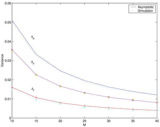
Figure 2: Average variance of channel estimates versus the coherence time $M$

Figure 2 shows the average variance of the channel estimates versus the coherence time $M$ with the configuration of $\beta=0.2$, $L=5$, $M_{t}=0$, $P_{e}=0.1$ and the signal-to-noise ratio (SNR)$=5$dB. The asymptotic results obtained from (23) and the simulation results for finite systems ($N=100$) with spreading codes for the shifted model are represented by solid and dotted curves, respectively. In this figure, the estimation error variance caused by decision feedback and noise are denoted by $\Delta_{f}$ and $\Delta_{n}$, respectively. The corresponding asymptotic results are obtained from the first and the second terms in (23), respectively. We can observe that the asymptotic results match the simulation results well even when $M$ is small. This figure also demonstrates the validity of results based on the independence assumption of the spreading codes given in Section II.A.

VI-B Normality of PIC Output

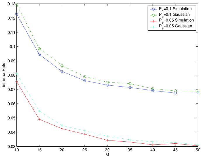
Figure 3: Comparison of simulated bit error rates and those obtained using a Gaussian approximation

Figure 3 shows the channel symbol error rate with the configuration of $\mbox{SNR}=10$dB, $K=N=30$ and $P_{e}=0.1$ and $0.05$. The solid curves represent the results obtained from numerical simulations and the dashed curves represent the results with the assumption that the output of PIC is CSCG distributed. The gap between the numerical results and CSCG based prediction is small, thus justifying the normality assumption of the PIC output.

VI-C User Capacity

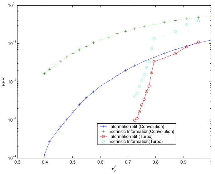
Figure 4: Performance of channel codes used in the numerical results, where the input SNR = $\frac{1}{\sigma_{n}^{2}}$

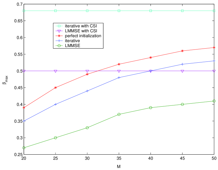
Figure 5: Maximum load of systems with convolutional codes

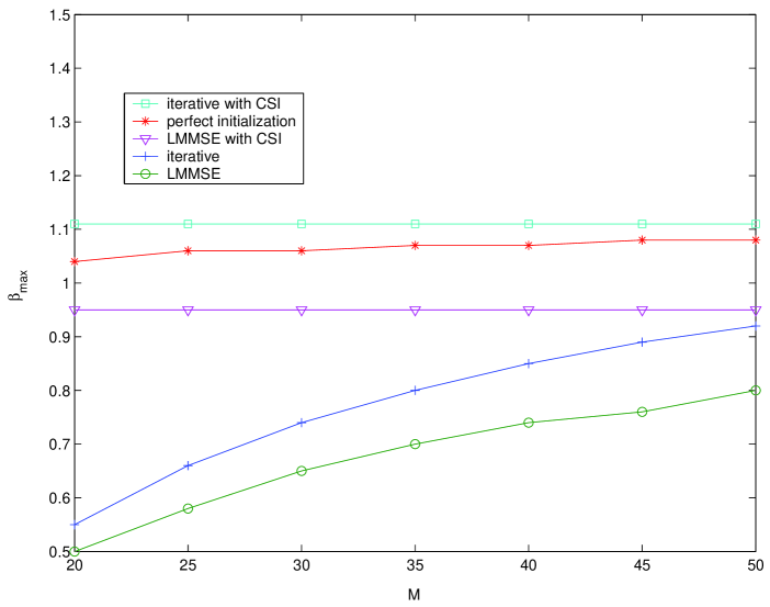
Figure 6: Maximum load of systems with turbo codes

We define the user capacity to be the maximum system load $\beta_{max}$ with which the system can achieve the information bit error rate of $10^{-3}$. Two types of channel codes, the convolutional code $(35,23)_{8}$ and a turbo code (with two constituent codes $(37,21)_{8}$), with bit rate $R=\frac{1}{2}$ and codeword length 1024 are used in this paper and their error rates for both information bits and extrinsic information based channel symbols are shown in Figure 4. The corresponding $\beta_{max}$’s for various values of coherence time $M$, denoted by ‘iterative’, are given in Figure 5 and Figure 6 for convolutional codes and turbo codes, respectively, with the configuration $\alpha=0.2$, SNR$=5$dB and $L=5$. The $\beta_{max}$’s of the non-iterative LMMSE detector, denoted by ‘LMMSE’, are given for comparison. We can see that the iterative system achieves substantially higher user capacity than the non-iterative one. The performance of systems with ideal initialization, where actual channel parameters are provided by a genie in the initialization stage, denoted by ‘Perfect initialization’, implies that a good initialization can improve the performance considerably. Thus, blind or semi-blind non-iterative techniques, which make use of information symbols, can be applied to obtain a better initialization. For comparison, the user capacities of both iterative and non-iterative systems with perfect channel state information are also given in both figures. An interesting observation is that the relative performance gain of iterative systems over the non-iterative ones is smaller for turbo codes than for convolutional codes. This is due to the steeper waterfall region in turbo codes.

VII Conclusions

In this paper, we have analyzed the performance of decision feedback based iterative channel estimation and multiuser detection in multipath DS-CDMA channels. The decoding process has been described as an iterative mapping in terms of the variance of the channel decoder output, and conditions assuring the convergence and uniqueness of a fixed point have been proposed. Numerical results show that the initialization is important to the iterations, thus necessitating the use of non-iterative blind or semi-blind channel estimation algorithms for initialization purposes. Another observation of interest is that the gain of the iterative process over a non-iterative one is small when a near-optimal channel coding scheme is used.

Appendix A Validity of Independence Model for Spreading Codes

In (1), for different values of $l$ and $m$, $\mathbf{s}_{kl}$ and $\mathbf{s}_{km}$ are generated by the same binary sequence with different offsets. Our purpose is to show that if $K$ and $N$ are large enough, we can regard the shifted spreading codes of different paths of a given user as independent sequences. The properties based on this assumption, which are used for the system performance analysis in this paper, include:

• The properties of crosscorrelation $\rho_{klmn}$ in Section II.A.

• The distribution of the eigenvalues of the matrix $\mathbf{S}\mathbf{S}^{T}$, when developing the expression of $\Delta_{n}$ for finite $M$ and large $K$ in Section III.C. Our assumption means that the corresponding distribution of the shifted model is asymptotically identical to that of the independent model.

It is easy to check the first item using the symmetry of the binary distribution. However, the validity of the second one is non-trivial and is of considerable importance when applying the theory of large random matrices to multipath fading channels. We can tackle this problem by showing that the moments of the eigenvalues in both models are the same via the following lemma.

Lemma A.1

Denote a generic eigenvalue of $\mathbf{S}\mathbf{S}^{T}$ by $\lambda$. Then the $m$-th moment of $\lambda$ in the shifted model is given by

$$E\left\{\lambda^{m}\right\}=\sum_{k=1}^{m}\left(\beta^{\prime}\right)^{k}\sum_{m_{1}+...+m_{k}=m}c(m_{1},...,m_{k}),\qquad\mbox{as }K\rightarrow\infty,$$

which is the same expression of that of the independent model, and where the definition of $c(m_{1},...,m_{k})$ is given in  [19] and $\beta^{\prime}=\frac{LK}{MN}$.

Proof:

Using similar arguments to those in [19], we have

$$\frac{1}{N}E\left\{\mbox{trace}\{(\mathbf{S}\mathbf{S}^{T})^{m}\}\right\}$$ (38)

$$= \frac{1}{N^{m+1}}\sum_{i_{1},...,i_{m}=1}^{K}\sum_{j_{1},...,j_{m}=1}^{N}E\{V_{i_{m},j_{1}}V_{i_{1},j_{1}}...V_{i_{m-1},j_{m}}V_{i_{m},j_{m}}\},$$

where $V_{i,j}=\sqrt{N}\mathbf{S}_{ij}$.

For any $i_{r}\neq i_{s}$, $V_{i_{r},j_{p}}=V_{i_{s},j_{q}}$ when $\lceil\frac{i_{r}}{L}\rceil=\lceil\frac{i_{s}}{L}\rceil$ and $j_{p}-j_{q}$ equals the offset difference between these two shifted sequences. However, the probability of such events vanishes as $K\rightarrow\infty$ since

$$P\left(|i_{r}-i_{s}|<L\right)\leq\left(\begin{array}[]{c}m\\ 2\\ \end{array}\right)\frac{2L+1}{KL}\rightarrow 0,\qquad\mbox{as }K\rightarrow\infty.$$ (41)

Thus, as $K\rightarrow\infty$, the term involving $V_{i,j}$’s of different users, which are mutually independent, dominates the summation in (38). The remaining part of the proof is the same as in  [19]. ∎

The following lemma (Theorem 30.1 in [5]) provides a sufficient condition for the equality of two probability measures when their moments are identical .

Lemma A.2

Let $\mu$ be a probability measure on the real line having finite moments $\alpha_{k}=\int_{-\infty}^{\infty}x^{k}\mu(dx)$ of all orders. If the power series $\sum_{k=1}^{\infty}\alpha_{k}\frac{r^{k}}{k!}$ has a positive radius of convergence, then $\mu$ is the only probability measure with the moments $\left\{\alpha_{m}\right\}_{m=1,2,...}$.

For applying Lemma I.2, we need the following lemma which provides an upper bound for the moments of the eigenvalues.

Lemma A.3

For any eigenvalue $\lambda$ of $\mathbf{S}\mathbf{S}^{T}$, there exists a constant $C>\max(1,\beta^{\prime})$ such that for $m=1,2,...$

$$E\left\{\lambda^{m}\right\}<C^{m}m^{m-2}.$$ (42)

Proof:

The result follows by induction on $m$.

It is easy to verify that (42) holds when $m=1,2$. Suppose $E\left\{\lambda^{n}\right\}<C^{n}n^{n-2}$, for $n=1,2,...,m$. Use the following recursive formula [19] to evaluate $E\left\{\lambda^{m+1}\right\}$, which is given by

$$E\left\{\lambda^{m+1}\right\}=\sum_{k=1}^{m+1}\beta^{\prime}\sum_{m_{1}+...+m_{k}=m+1}E\left\{\lambda^{m_{1}-1}\right\}\cdots E\left\{\lambda^{m_{k}-1}\right\}.$$

Then we have

$$E\left\{\lambda^{m+1}\right\} = \beta^{\prime}\left(1+mE\{\lambda\}+E\{\lambda^{m}\}+\sum_{k=2}^{m-1}\sum_{m_{1}+...+m_{k}=m+1}E\left\{\lambda^{m_{1}-1}\right\}...E\left\{\lambda^{m_{k}-1}\right\}\right)$$ (45)

$$< \beta^{\prime}\left(1+m\beta^{\prime}+C^{m}m^{m-2}+\sum_{k=2}^{m-1}\sum_{m_{1}+...+m_{k}=m+1}\prod_{i=1}^{k}C^{m_{i}-1}m_{i}^{m_{i}-3}\right)$$

$$< \beta^{\prime}\left(1+m\beta^{\prime}+C^{m}m^{m-2}+\sum_{k=2}^{m-1}\sum_{m_{1}+...+m_{k}=m+1}C^{m+1-k}m^{m-1-k}\right)$$

$$< C^{m+1}\left(1+m^{m-1}+\sum_{k=2}^{m-1}\left(\begin{array}[]{ll}m\\ k-1\end{array}\right)m^{m-1-k}\right)$$

$$< C^{m+1}\left(1+m^{m-1}+\sum_{k=1}^{m-2}\left(\begin{array}[]{ll}m-1\\ k\end{array}\right)m^{m-1-k}\right)$$ (48)

$$= C^{m+1}\sum_{k=0}^{m-1}\left(\begin{array}[]{ll}m-1\\ k\end{array}\right)m^{m-1-k}$$

$$= C^{m+1}(1+m)^{m-1},$$

where the first inequality is based the assumption on $n=1,...,m$ and the fact that $E\{\lambda\}=\beta^{\prime}$; the third inequality applies the condition that $C>\max(1,\beta^{\prime})$ and $m^{m-1}>m^{m-2}+m$ for $m>2$. This concludes the proof. ∎

Applying Stirling’s formula and Lemmas I.1,2,3, we can obtain the conclusion that the eigenvalue distribution of $\mathbf{S}\mathbf{S}^{T}$ in the shifted model is identical to that of the independent model, thus assuring the assumption that the columns of $\mathbf{S}$ can be regarded as independent in the large system limit.

Appendix B Proof of Lemma III.2

Proof:

From the definition of $\delta{\mathbf{a}}_{f}$, we have

$$E\{\delta{\mathbf{a}}_{f}\}=-\frac{1}{M}\left(E\{\mathbf{S}^{T}\delta\mathbf{S}\mathbf{a}\}-E\{\delta\mathbf{S}^{T}\delta\mathbf{S}\mathbf{a}\}\right).$$ (52)

We consider the term $E\{\delta\mathbf{S}^{T}\delta\mathbf{S}\mathbf{a}\}$ first. It is easy to check that (recall that $\mathbf{s}_{kl}$ denotes the spreading code of user $k$ along path $l$)

$$\frac{1}{M}E\left\{\left(\delta\mathbf{S}^{T}\delta\mathbf{S}\right)_{ij}\right\} = \frac{1}{M}\sum_{m=1}^{M}\mathbf{s}^{T}_{pq}(m)\mathbf{s}_{rs}(m)E\left\{\delta b_{p}\delta b_{r}\right\}$$ (55)

$$= \left\{\begin{array}[]{ll}0,\qquad\mbox{if }p\neq r\\ \frac{4P_{e}}{M}\sum_{m=1}^{M}\mathbf{s}^{T}_{pq}(m)\mathbf{s}_{rs}(m),\qquad\mbox{if }p=r\end{array}\right.,$$

where $p=\left\lceil\frac{i}{L}\right\rceil$, $q=\mbox{mod}\left(i,L\right)$, $r=\left\lceil\frac{j}{L}\right\rceil$, $s=\mbox{mod}\left(j,L\right)$. It should be noted we applied the fact that $E\left\{\delta b_{p}\delta b_{r}\right\}=4P_{e}$ in the second equality.

According to Assumption II.3, the spread codes are mutually independent for different users or different paths. Thus, by applying the strong law of large numbers, we have

$$\frac{1}{M}\sum_{m=1}^{M}\mathbf{s}^{T}_{pq}(m)\mathbf{s}_{rs}(m)\rightarrow\left\{\begin{array}[]{ll}0,\qquad\mbox{if }(p,q)\neq(r,s)\\ 1,\qquad\mbox{if }(p,q)=(r,s)\end{array}\right..$$ (58)

Therefore, we have

$$\frac{1}{M}E\left\{\left(\delta\mathbf{S}^{T}\delta\mathbf{S}\right)_{ij}\right\}\rightarrow\left\{\begin{array}[]{ll}0,\qquad\mbox{if }i\neq j\\ \frac{4P_{e}}{M},\qquad\mbox{if }i=j\end{array}\right.,\qquad\mbox{almost surely, as }M\rightarrow\infty$$ (61)

Similarly, we can show that

$$\frac{1}{M}E\left\{\left(\mathbf{S}^{T}\delta\mathbf{S}\right)_{ij}\right\}\rightarrow\left\{\begin{array}[]{ll}0,\qquad\mbox{if }i\neq j\\ \frac{2P_{e}}{M},\qquad\mbox{if }i=j\end{array}\right.,\qquad\mbox{almost surely, as }M\rightarrow\infty$$ (64)

This completes the proof. ∎

Appendix C Proof of Prop. III.3

Proof:

The covariance matrix $\mathbf{\Sigma}_{f}$ is given by

$$\bf{\Sigma}_{f} \triangleq \frac{1}{M^{2}}\mbox{cov}\left(\hat{\mathbf{S}}^{T}\delta\mathbf{S}\mathbf{a}\right)$$ (65)

$$= \frac{1}{M^{2}}E\left\{{\mathbf{S}}^{T}\delta\mathbf{S}\mathbf{a}\mathbf{a}^{H}\delta\mathbf{S}^{T}{\mathbf{S}}\right\}-\frac{1}{M^{2}}E\left\{{\mathbf{S}}^{T}\delta\mathbf{S}\mathbf{a}\mathbf{a}^{H}\delta\mathbf{S}^{T}{\delta\mathbf{S}}\right\}$$

$$- \frac{1}{M^{2}}E\left\{\delta{\mathbf{S}}^{T}\delta\mathbf{S}\mathbf{a}\mathbf{a}^{H}{\delta\mathbf{S}}^{T}\mathbf{S}^{T}\right\}+\frac{1}{M^{2}}E\left\{\delta{\mathbf{S}}^{T}\delta\mathbf{S}\mathbf{a}\mathbf{a}^{H}\delta\mathbf{S}^{T}\delta{\mathbf{S}}\right\}$$

$$- E\{\delta{\mathbf{a}}_{f}\}E\{\delta{\mathbf{a}}_{f}\}^{H}.$$

The elements in ${\mathbf{S}}^{T}\delta\mathbf{S}\mathbf{a}\mathbf{a}^{H}\delta\mathbf{S}^{T}{\mathbf{S}}$ are given by

$$\left({\mathbf{S}}^{T}\delta\mathbf{S}\mathbf{a}\mathbf{a}^{H}\delta\mathbf{S}^{T}{\mathbf{S}}\right)_{ij}=\sum_{p=1}^{M}\sum_{q=1}^{M}\sum_{k=1}^{KL}\sum_{l=1}^{KL}{\tilde{\mathbf{s}}}_{i}^{T}(p)\delta\tilde{\mathbf{s}}_{k}(p){\tilde{\mathbf{s}}}_{j}^{T}(q)\delta{\tilde{\mathbf{s}}}_{l}(q)\textmd{a}_{k}\textmd{a}_{l}^{*},$$

where ${\tilde{\mathbf{s}}}_{i}(p)\triangleq b_{\lceil\frac{i}{L}\rceil}(p)\mathbf{s}_{\scriptsize\lceil\frac{i}{L}\rceil,\mbox{ mod}(i,L)}(p)$, namely the spreading code (incorporating the channel symbol) of the $\mbox{ mod}(i,L)$-th path of user $\lceil\frac{i}{L}\rceil$ at symbol period $p$, $\delta{\tilde{\mathbf{s}}}_{i}(p)\triangleq\delta b_{\lceil\frac{i}{L}\rceil}(p)\mathbf{s}_{\scriptsize\lceil\frac{i}{L}\rceil,\mbox{ mod}(i,L)}(p)$ and $\textmd{a}_{k}$ is the $k$-th element of vector $\mathbf{a}$ and equals $a_{\left\lceil\frac{k}{L}\right\rceil,mod(k,L)}$. To compute the corresponding expectation, we apply the following properties, which are based on Assumption II.4:

• When $p=q$, if $\lceil\frac{k}{L}\rceil=\lceil\frac{l}{L}\rceil$, $P(\delta\tilde{\mathbf{s}}_{k}(p)\neq 0,\delta\tilde{\mathbf{s}}_{l}(q)\neq 0)=P_{e}$, since $\delta\tilde{\mathbf{s}}_{k}(p)$ and $\delta\tilde{\mathbf{s}}_{l}(p)$ are determined by the same decision feedback;

• When $p=q$, if $\lceil\frac{k}{L}\rceil\neq\lceil\frac{l}{L}\rceil$, $P(\delta\tilde{\mathbf{s}}_{k}(p)\neq 0,\delta\tilde{\mathbf{s}}_{l}(q)\neq 0)=P_{e}^{2}$, since $\delta\tilde{\mathbf{s}}_{k}(p)$ and $\delta\tilde{\mathbf{s}}_{l}(p)$ are determined by decision feedback from different users;

• When $p\neq q$, $P(\delta\tilde{\mathbf{s}}_{k}(p)\neq 0,\delta\tilde{\mathbf{s}}_{l}(q)\neq 0)=P_{e}^{2}$, since $\delta\tilde{\mathbf{s}}_{k}(p)$ and $\delta\tilde{\mathbf{s}}_{l}(p)$ are determined by decision feedback from different symbol periods;

• When $\delta\tilde{\mathbf{s}}_{k}(p)\neq 0$, $\delta\tilde{\mathbf{s}}_{k}(p)=2{\tilde{\mathbf{s}}}_{k}(p)$.

Thus the expectation of $i-j$th element of ${\mathbf{S}}^{T}\delta\mathbf{S}\mathbf{a}\mathbf{a}^{H}\delta\mathbf{S}^{T}{\mathbf{S}}$ is given by

$$E\left\{\left({\mathbf{S}}^{T}\delta\mathbf{S}\mathbf{a}\mathbf{a}^{H}\delta\mathbf{S}^{T}{\mathbf{S}}\right)_{ij}\right\}$$

$$= 4P_{e}\sum_{p=1}^{M}\sum_{k=1}^{KL}\sum_{\lceil\frac{l}{L}\rceil=\lceil\frac{k}{L}\rceil}{\tilde{\mathbf{s}}}_{i}^{T}(p){\tilde{\mathbf{s}}}_{k}(p){\tilde{\mathbf{s}}}_{j}^{T}(p){\tilde{\mathbf{s}}}_{l}(p)\textmd{a}_{k}\textmd{a}_{l}^{*}$$

$$+ 4P_{e}^{2}\sum_{p=1}^{M}\sum_{k=1}^{KL}\sum_{\lceil\frac{l}{L}\rceil\neq\lceil\frac{k}{L}\rceil}{\tilde{\mathbf{s}}}_{i}^{T}(p){\tilde{\mathbf{s}}}_{k}(p){\tilde{\mathbf{s}}}_{j}^{T}(p){\tilde{\mathbf{s}}}_{l}(p)\textmd{a}_{k}\textmd{a}_{l}^{*}$$

$$+ 4P_{e}^{2}\sum_{\scriptsize\begin{array}[]{ll}p,q=1\\ p\neq q\end{array}}^{M}\sum_{k=1}^{KL}\sum_{l=1}^{KL}{\tilde{\mathbf{s}}}_{i}^{T}(p){\tilde{\mathbf{s}}}_{k}(p){\tilde{\mathbf{s}}}_{j}^{T}(q){\tilde{\mathbf{s}}}_{l}(q)\textmd{a}_{k}\textmd{a}_{l}^{*}$$

$$= T_{1}+T_{2}+T_{3},$$

where $T_{1}$, $T_{2}$ and $T_{3}$ represent the corresponding three summations, respectively.

Applying the strong law of large numbers and the assumption on the spreading codes that $\left\{{\tilde{\mathbf{s}}}_{i}(p)\right\}$ are independent for different values of $i$ or $p$, we can obtain that, as $M\rightarrow\infty$, the following conclusions hold almost surely:

$$\frac{1}{M}T_{1} \rightarrow \left\{\begin{array}[]{lll}4P_{e}\left(|\textmd{a}_{i}|^{2}+\frac{1}{N}\sum_{k=1\mbox{, }k\neq i}^{KL}|\textmd{a}_{k}|^{2}\right),\qquad\mbox{if }i=j,\\ 4P_{e}\left(1+\frac{1}{N}\right)\textmd{a}_{i}\textmd{a}_{j}^{*},\qquad\mbox{if }i\neq j\mbox{ and }\lceil\frac{i}{L}\rceil=\lceil\frac{j}{L}\rceil,\\ 0,\qquad\mbox{if }\lceil\frac{i}{L}\rceil\neq\lceil\frac{j}{L}\rceil\end{array}\right.$$ (72)

$$\frac{1}{M}T_{2} \rightarrow \left\{\begin{array}[]{ll}4P_{e}^{2}\left(1+\frac{1}{N}\right)\textmd{a}_{i}\textmd{a}_{j}^{*},\qquad\mbox{if }\lceil\frac{i}{L}\rceil\neq\lceil\frac{j}{L}\rceil,\\ 0,\qquad\mbox{if }\lceil\frac{i}{L}\rceil=\lceil\frac{j}{L}\rceil\end{array}\right.$$ (75)

$$\frac{1}{M^{2}}T_{3} \rightarrow 4P_{e}^{2}\textmd{a}_{i}\textmd{a}_{j}^{*},\qquad\forall i,j.$$

We can apply the same manipulation and obtain that $E\left\{{\mathbf{S}}^{T}\delta\mathbf{S}\mathbf{a}\mathbf{a}^{H}\delta\mathbf{S}^{T}{\delta\mathbf{S}}\right\}=E\left\{\delta{\mathbf{S}}^{T}\delta\mathbf{S}\mathbf{a}\mathbf{a}^{H}{\delta\mathbf{S}}^{T}\mathbf{S}\right\}=\frac{1}{2}E\left\{\delta{\mathbf{S}}^{T}\delta\mathbf{S}\mathbf{a}\mathbf{a}^{H}\delta\mathbf{S}^{T}\delta{\mathbf{S}}\right\}$ as $M\rightarrow\infty$. Therefore, we can obtain (20) since the sum of the middle three terms in (65) is zero and $T_{3}$ cancels $E\{\delta{\mathbf{a}}_{f}\}E\{\delta{\mathbf{a}}_{f}\}^{H}$. ∎

It should be noted that the above analysis is also valid for asynchronous case when $P_{e}$ is sufficiently small. Similar to the discussion in Section III.A, we can remove part of the chips in the first and the last symbol periods to obtain a similar matrix $\mathbf{S}_{NM-d_{max}\times KL}$, where $d_{max}$ denotes the largest time offsets of different users, measured in chips. When $P_{e}$ is sufficiently small and $M$ is sufficiently large, we can ignore the terms scaled by $P_{e}^{2}$ and the edge effect in the first and last symbol period. Then, we have

$$E\left\{\left({\mathbf{S}}^{T}\delta\mathbf{S}\mathbf{a}\mathbf{a}^{H}\delta\mathbf{S}^{T}{\mathbf{S}}\right)_{ij}\right\}\approx 4P_{e}\sum_{k=1}^{KL}\sum_{\lceil\frac{l}{L}\rceil=\lceil\frac{k}{L}\rceil}{\tilde{\mathbf{s}}}_{i}^{T}{\tilde{\mathbf{s}}}_{k}{\tilde{\mathbf{s}}}_{j}^{T}{\tilde{\mathbf{s}}}_{l}\textmd{a}_{k}\textmd{a}_{l}^{*},$$

where $\tilde{\mathbf{s}}_{k}$ is the $k$-th column of matrix $\mathbf{S}$, which converges to $T_{1}$ as $M\rightarrow\infty$.

Figure 1: CDMA system with an iterative receiver

References

• [1] P. Alexander, A. Grant and M. C. Reed, “Iterative detection of code-division multiple-acess with error control coding,” European Trans. Telecommun., Vol. 9, pp. 419–426, Aug. 1998.
• [2] P. Alexander and A. Grant, “Iterative channel and information sequence estimation in CDMA,” Proceedings of IEEE Sixth International Symposium on Spread Spectrum Techniques and Applications, pp. 593–597, Parsippany, NJ, Sept. 2000.
• [3] Z. D. Bai, J. W. Silverstein and Y. Q. Yin, “A note on the largest eigenvalue of a large dimensional sample covariance matrix ,” Journal Multivariate Anal., Vol. 26, pp. 166–168, 1998.
• [4] L. R. Bahl, J. Cocke, F. Jelinek and J. Raviv, “Optimal decoding of linear codes for minimizing symbol error rate,” IEEE Trans. Inform. Theory, Vol. 20, pp. 284–287, Aug. 1974.
• [5] P. Billingsley, Probability and Measure. John Wiley and Sons Inc, New York, US, 1995.
• [6] S. Buzzi and H. V. Poor, “Channel estimation and multiuser detection in long-code DS/CDMA systems,” IEEE J. Select. Areas Commun., Vol. 19, pp. 1476–1487, Aug. 2001.
• [7] S. Buzzi, M. Lops and S. Sardellitti, “Performance of iterative data detection and channel estimation for single-antenna and multiple-antenna wireless communications,” Proceedings of 2003 Asilomar Conference on Signals, Systems, and Computers, Pacific Grove, CA, 2003.
• [8] S. Buzzi, and H. V. Poor, “A multi-pass approach to joint data and channel estimation in long-code CDMA systems,” IEEE Trans. Wireless Commun., Vol. 3, pp. 612–626, March, 2004.
• [9] J. Evans and D. N. C. Tse, “Large system performance of linear multiuser receivers in multipath fading channels,” IEEE Trans. Inform. Theory, Vol. 46, pp. 2059–2078, Aug. 2000.
• [10] G. H. Golub and C. F. Van Loan, Matrix Computations. The Johns Hopkins University Press, Baltimore, MD, 1983.
• [11] R. A. Horn and C. R. Johnson, Matrix Analysis. Cambridge University Press, Cambridge, UK, 1985.
• [12] J. Hou, J. E. Smee, H. D. Pfister and S. Tomasin, “Implementing interference cancellation to increase the EV-DO Rev A reverse link capacity,” IEEE Commun. Mag., Vol. 44, pp. 96–102, Feb. 2006.
• [13] M. Kobayashi, J. Boutros and G. Caire, “Successive interference cancellation with SISO decoding and EM channel estimation,” IEEE J. Select. Areas Commun., Vol. 19, pp. 1450–1460, Aug. 2001.
• [14] E. Kreyszig, Introductory Functional Analysis With Applications. John Wiley and Sons Inc, New York, 1989.
• [15] A. Lampe, “Iterative multiuser detection with integrated channel estimation for coded DS-CDMA,” IEEE Trans. Commun., Vol. 50, no. 8, pp. 1217–1223, Aug. 2002.
• [16] C. Laot, A. Glavieux and J. Labat, “Turbo equalization: Adaptive equalization and channel decoding jointly optimized,” IEEE J. Select. Areas Commun., Vol. 19, pp. 1744–1752, Sept. 2001.
• [17] H. Li and H. V. Poor, “Performance of channel estimation in long code DS-CDMA with and without decision feedback,” Proceedings of the 2003 Conference on Information Sciences and Systems, The Johns Hopkins University, Baltimore, MD, March 2003.
• [18] H. Li and H. V. Poor, “Impact of channel estimation error on multiuser detection via the replica method,” EURASIP Journal on Wireless Communicaitons and Networking, Vol.2005, pp. 175–186, May 2005.
• [19] L. Li, A. M. Tulino and S. Verdú, “Asymptotic eigenvalue moments for linear multiuser detection,” Communications in Information and Systems, Vol.1, no. 3, pp. 273 – 304, Sept. 2001.
• [20] M. Loncar, R. Müller, J. Wehinger, C. Mecklenbraeuker, and T. Abe, “Iterative channel estimation and data detection in frequency-selective fading MIMO channels,” European Transactions on Telecommunications, Vol.15, no.53, pp.459–470, Sept./Oct. 2004.
• [21] R. Lupas and S. Verdú, “Linear multiuser detectors for synthronous code-division multiple-acess channels,” IEEE Trans. Inform. Theory, Vol. 35, pp. 123–136, Aug. 1989.
• [22] M. Moher, “An iterative multiuser decoder for near capacity communications,” IEEE Trans. Commun., Vol. 46, no.7, pp. 870–880, July 1998.
• [23] H. Niu and J. A. Ritcey, “Iterative channel estimation and decoding of pilot symbol assisted LDPC coded QAM over flat fading channels,” Proceedings of 2003 Asilomar Conference on Signals, Systems, and Computers, Pacific Grove, CA, 2003,
• [24] H. V. Poor, “Iterative multiuser detection,” IEEE Signal Processing Magazine, Vol. 21, No,1, pp. 81–86, 2004.
• [25] R. Raheli, A. Polydoros, and C. Tzou, “Per-survivor processing: A general approach to MLSE in uncertain environments,” IEEE Trans. Commun., Vol. 43, pp. 354–364, Feb./March/April, 1995.
• [26] M. C. Reed, C. B. Schlegel, P. D. Alexander and J. A. Asenstorfer, “Iterative multiuser detection for CDMA with FEC: Near single user performance,” IEEE Trans. Commun., Vol. 46, no.12, pp. 1693–1699, Dec. 1998.
• [27] M. C. Valenti and B. D. Woerner, “Iterative multiuser detection for convolutionally coded asynchronous DS-CDMA,” in IEEE Int. Symp. Personal, Indoor, Mobile Radio Commun., Boston, Sept. 1998.
• [28] S. Verdú, “Minimum probability of error for asynchronous Gaussian multiple-access channels,” IEEE Trans. Inform. Theory, Vol. 32, pp. 85–96, Jan. 1986.
• [29] S. Verdú, Multiuser Detection. Cambridge University Press, Cambridge, UK, 1998.
• [30] X. Wang and H. V. Poor, Wireless Communication Systems: Advanced Techniques for Signal Reception. Prentice-Hall, Upper Saddle River, NJ, 2004.
• [31] X. Wang and H. V. Poor, “Iterative (turbo) soft interference cancellation and decoding for coded CDMA,” IEEE Trans. Commun., Vol. 47, no.7, pp. 1046–1061, July 1999.
• [32] X. Wang and H. V. Poor, “Subspace methods for blind channel estimation and multiuser detection in CDMA systems,” Wireless Networks, Vol. 6, pp. 59–71, Feb. 2000.
• [33] Z. Xu and M. K.Tsatsanis, “Blind channel estimation for long code multiuser CDMA systems,” IEEE Trans. Signal Processing, Vol. 48, pp. 988–1001, Apr. 2000.
Refer to caption