Good Illumination of Minimum Range

Abstract

A point $p$ is 1-well illuminated by a set $F$ of $n$ point lights if $p$ lies in the interior of the convex hull of $F$. This concept corresponds to $\triangle$-guarding [14] or well-covering [9]. In this paper we consider the illumination range of the light sources as a parameter to be optimized. First, we solve the problem of minimizing the light sources’ illumination range to 1-well illuminate a given point $p$. We also compute a minimal set of light sources that 1-well illuminates $p$ with minimum illumination range. Second, we solve the problem of minimizing the light sources’ illumination range to 1-well illuminate all the points of a line segment with an $\mathcal{O}(n^{2})$ algorithm. Finally, we give an $\mathcal{O}(n^{2}\log n)$ algorithm for preprocessing the data so that one can obtain the illumination range needed to 1-well illuminate a point of a line segment in $\mathcal{O}(\log n)$ time. These results can be applied to solve problems of 1-well illuminating a trajectory by approaching it to a polygonal path.

M. Abellanas ^{† 1}, A. Bajuelos ², G. Hern ndez ¹ F. Hurtado ³, I. Matos ², B. Palop ⁴

¹ Universidad Polit cnica de Madrid, ² Universidade de Aveiro,

³ Universitat Polit cnica de Catalunya, ⁴ Universidad de Valladolid

^† mabellanas@fi.upm.es, corresponding author

Key words: Computational Geometry, Limited Illumination Range, Visibility, Good Illumination

1 Introduction and definitions

Visibility or illumination has been the main topic for a lot of different works but most of them cannot be applied to real life, since they deal with ideal concepts. For instance, light sources have some restrictions since they cannot illuminate an infinite region as their light naturally fades as the distance grows. As well as cameras or robot vision systems, both have severe visibility range restrictions because they cannot observe with sufficient detail far away objects. We present some of these illumination problems adding several restrictions to make them more realistic, each light source has a limited illumination range so their illuminated regions are delimited. We use a limited visibility definition due to Ntafos [13] as well as a new concept related to this type of problems, the t-good illumination due to Canales et. al [1, 6]. This last concept tests the light sources’ distribution in the plane. If they are somehow surrounding the object we want to illuminate, there is a big chance it is $1$-well illuminated (1-good illumination is also known as $\triangle$-guarding [14] or well-covering [9]).

This paper is solely focused in an optimization problem related to limited 1-good illumination. We propose the linear algorithm MER-Point to calculate the Minimum Embracing Range (MER) of a point in the plane and it also solves the decision problem. We move on to the computation of the MER of a line segment. In order to do this, we propose an algorithm that takes advantage of the Parametric Search [10, 11] and runs in $\mathcal{O}(n^{2})$ time. Our last algorithm is the main result in this paper as it computes the E-Voronoi diagram [3] restricted to a line segment which allows us to obtain the illumination range needed to 1-well illuminate a query point of the line segment in $\mathcal{O}(\log n)$ time.

Let $F$ be a set of $n$ light sources in the plane that we call sites. Each light source $f_{i}\in F$ has limited illumination range $r>0$, this is, they can only illuminate objects that are within the circle centered at $f_{i}$ with radius $r$. As we only consider $1$-good illumination, throughout this paper we will refer to it just as illumination. The first two problems minimize the light sources’ range while illuminating certain objects (points and line segments). On the third one, we also try to answer efficiently which light source embraces any given point in a line segment, this is, we want to compute the E-Voronoi Diagram restricted to a line segment. The next definitions follow from the notation introduced by Chiu and Molchanov [8], where CH$(F)$ denotes the convex hull of the set $F$.

Definition 1.1

A set of points $F$ is called an embracing set for a point $p$ in the plane if $p$ lies in the interior of the $\mathrm{CH}(F)$.

Definition 1.2

A site $f_{i}\in F$ is an embracing site for $p$ if $p$ is an interior point of the convex hull formed by $f_{i}$ and by all the sites of $F$ closer to $p$ than $f_{i}$.

Following this definition, there may be more than one embracing site for a point $p$. Since we are trying to minimize the light sources’ illumination range, in fact, we are trying to compute the closest embracing site for point $p$ (see Figure 1). The NNE-graph [8] consists of a set of vertices $V$ where each vertex $v\in V$ is connected to its first nearest neighbour, its second nearest neighbour, …, until $v$ is in the convex hull of its nearest neighbours. Chan et al. [7] present several algorithms to construct the NNE-graph.

Figure 1: The light sources $f_{1}$ and $f_{5}$ are embracing sites for point $p$. The light source $f_{5}$ is the closest embracing site for $p$ with illumination range $r=d(p,f_{5})$.

Definition 1.3

Let $F$ be a set of $n$ light sources in the plane. We call Closest Embracing Triangle for a point $p$, $\mathrm{CET}(F,p)$, to a set of three light sources of $F$ containing $p$ in the interior of the triangle they define and where one of the three light sources is the closest embracing site for $p$.

Since the set of light sources is always $F$, CET($F,p$) is shortened to CET($p$) in this paper.

Definition 1.4 ([6])

Let $F$ be a set of $n$ light sources in the plane. We say that a point $p$ in the plane is $t$-well illuminated by $F$ if every open half-plane containing $p$ in its interior, contains at least $t$ light sources of $F$ illuminating $p$.

This definition tests the light sources’ distribution in the plane so that the greater the number of light sources in every open half-plane containing the point $p$, the better the illumination of $p$. This concept can also be found under the name of $\triangle$-guarding [14] or well-covering [9]. The motivation behind this definition is the fact that, in some applications, it is not sufficient to have one point illuminated but some neighbourhood of it [9].

Let $C(f_{i},r)$ be the circle centered at $f_{i}$ with radius $r$ and let $A_{r}(f_{1},f_{2},f_{3})$ denote illuminated area by the light sources $f_{1},f_{2}$ and $f_{3}$ (see Figure 2(a)). It is easy to see that $A_{r}(f_{1},f_{2},f_{3})=C(f_{1},r)\cap C(f_{2},r)\cap C(f_{3},r)$. We use $A_{r}^{E}(f_{1},f_{2},f_{3})=A_{r}(f_{1},f_{2},f_{3})\cap\mathrm{int}(\mathrm{CH}(f_{1},f_{2},f_{3}))$ to denote the illuminated area embraced by the light sources $f_{1},f_{2}$ and $f_{3}$.

Figure 2: (a) $A_{r}^{E}(f_{1},f_{2},f_{3})$ is the shaded open area, so every point that lies inside it is 1-well illuminated by the light sources $f_{1},f_{2}$ and $f_{3}$. (b) All the interior points of the $\mathrm{CH}(f_{1},f_{2},f_{3})$ are 1-well illuminated since $r\geq\max\{d(f_{i},f_{j}),f_{i}\neq f_{j}\in\{f_{1},f_{2},f_{3}\}\}$.

Definition 1.5

We say that a point $p$ is $1$-well illuminated by the light sources $f_{1},f_{2}$ and $f_{3}$ if $p\in A_{r}^{E}(f_{1},f_{2},f_{3})$ for some range $r>0$.

Definition 1.6

Given a set $F$ of $n$ light sources, we call Minimum Embracing Range to the minimum range needed to 1-well illuminate a point $p$ or a set of points $S$ in the plane, respectively $\mathrm{MER}(F,p)$ or $\mathrm{MER}(F,S)$.

Since the set $F$ is clear from the context, we will use “MER of a point $p$” instead of MER($F,p$) and “MER of a set $S$” instead of MER($F,S$). Once we have found the closest embracing site for a point, its MER is given by the distance between the point and its closest embracing site. So we know that a point is 1-well illuminated if all the light sources’ illumination range is, at leat, the same value as MER. In the next section we focus on our solution to obtain the closest embracing site of $F$ for a point $p$ as well as one CET($p$).

2 Minimum Embracing Range of a Point

Let $F$ be a set of $n$ light sources in the plane and $p$ a point we want to 1-well illuminate. The objective of this section is to compute the value of the MER of $p$, $r_{m}$, as well as one CET($p$). The closest embracing site for $p$ can be obtained in linear time using the NNE-graph by Chan et. al [7]. The algorithm we present in this section also has the same time complexity.

The MER-Point Algorithm

First of all, we compute the distances from $p$ to all the light sources. Afterwards, we compute the median of all the distances in linear time [4]. Depending on this value, we can split the light sources in two halves: the set $F_{c}$ that contains the closest half to $p$ and the set $F_{f}$ that contains the furthest half. We check whether $p\in\mathrm{int}(\mathrm{CH}(F_{c}))$, what is equivalent to test if $F_{c}$ is an embracing set for $p$. If the answer is negative, we recurse adding the closest half in $F_{f}$. Otherwise, we recurse halving $F_{c}$. This logarithmic search runs until we find the light source $f_{p}\in F$ and the subset $F^{E}\subseteq F$ such that $p\in\mathrm{int}(\mathrm{CH}(F^{E}))$ but $p\notin\mathrm{int}(\mathrm{CH}(F^{E}\setminus\{f_{p}\})$. The light source $f_{p}$ is the closest embracing site for $p$ and its MER is $r_{m}=d(f_{p},p)$.

On each recursion, we have to check whether $p\in\mathrm{int}(\mathrm{CH}(F^{\prime})),F^{\prime}\subseteq F$. This can be done in linear time [12] if we choose carefully the set of points so that each point is studied only once. As soon as we have computed $f_{p}$, we can find the two other vertices of a CET$(p)$ in linear time as follows. Consider the circle centered at $p$ of radius $r_{m}$ and the line $pf_{p}$ that splits the light sources inside the circle in two sets. Note that if $f_{p}$ is the closest embracing site for $p$ then there is a semicircle empty of other light sources than $f_{p}$. A CET$(p)$ has $f_{p}$ and two other light sources in the circle as vertices. Actually, any pair of light sources $f_{l},f_{r}$ such that each lies on a different side of the line passing through $p$ and $f_{p}$ verifies that $p\in\mathrm{int(CH}(f_{l},f_{p},f_{r}))$.

Proposition 2.1

Given a set $F$ of $n$ light sources with limited illumination range and a point $p$ in the plane, the algorithm MER-Point computes the MER of $p$ and a $\mathrm{CET}(p)$ in $\mathcal{O}(n)$ time.

Proof: Let $F$ be a set of $n$ light sources. The distances from $p$ to all the light sources can be computed in linear time. Computing the median also takes linear time [4], as well as splitting $F$ in two halves. Checking if $p\in\mathrm{int}(\mathrm{CH}(F^{\prime})),F^{\prime}\subseteq F$, is linear on the number of light sources in $F^{\prime}$. So the total time for this logarithmic search is $\mathcal{O}(n+\frac{n}{2}+\frac{n}{4}+\frac{n}{8}+...)=\mathcal{O}(n)$. Therefore, we find the closest embracing site for $p$ in linear time. So this algorithm computes the MER of $p$ and a $\mathrm{CET}(p)$ in total $\mathcal{O}(n)$ time. $\square$

The decision problem is trivial after the MER of $p$ is computed. Point $p$ is 1-well illuminated if the given illumination range is greater or equal to the MER of $p$.

3 Minimum Embracing Range of a Line Segment

In this section we compute the MER, $r_{m}$, of a line segment, this is, we compute the minimum illumination range needed to 1-well illuminate a line segment with a set of light sources. Without loss of generality, suppose that a line segment $s=\overline{p_{l}p_{r}}$ is an horizontal line segment and that $p_{l}$ and $p_{r}$ are respectively the leftmost and the rightmost points of $s$. Since our solution uses the Parametric Search technique due to Megiddo [10, 11], we first concentrate on the following decision problem: given a range $r>0$, is $s$ 1-well illuminated by a set $F$ of $n$ light sources?

The algorithm in this section decides if a line segment $s$ is 1-well illuminated knowing that the light sources of $F$ have illumination range $r$. The idea behind this algorithm is to split $s$ into several open segments and check if $r$ is enough to 1-well illuminate all of them. We will show that, if two consecutive open segments are 1-well illuminated, the point in between also is. Hence, if all segments and both extreme points are 1-well illuminated, so is the segment $s$.

Let us first introduce some notation. We know that each light source $f_{i}\in F$ illuminates a circle centered at itself with radius $r$, $C(f_{i},r)$, and that each circle can intersect $s$ in at most two points. Since we have $n$ light sources, there are $n$ such circles and at most $2n$ intersection points between $s$ and the circles. Let $I$ be the set containing the points $p_{l}=i_{0}$ and $p_{r}=i_{m}$ and all the sorted intersection points according to their $x$-coordinate $i_{1}\dots i_{m-1}$.If $i_{k}$ is an intersection point between $C(f_{i},r)$ and $s$, let $f(i_{k})$ be $f_{i}$. If $i_{k}\in I$ is to the left (resp. right) of $f(i_{k})$, it is called the leftmost (rightmost) intersection point. Let also $s_{k}=(i_{k-1},i_{k})$, with $i_{k-1},i_{k}\in I$ be the open segment between the intersection points $i_{k-1}$ and $i_{k}$, for $k=1,\ldots,m$. Note that the light sources illuminating $s_{k}$ are the same for all points in $s_{k}$ since its endpoints are consecutive intersections of $I$. The function $\mathcal{F}(s_{k})$ returns the set of the light sources that illuminate $s_{k}\subseteq s$ with range $r$. Knowing that $\mathcal{F}(s_{1})=\mathcal{F}(i_{0})$, the function is recursively defined for $k=1,\ldots,m-1$ as follows.

$$\mathcal{F}(s_{k+1})=\left\{\begin{array}[]{ll}\mathcal{F}(s_{k})\cup\{f(i_{k})\},&\textrm{if $i_{k}$ is a leftmost intersection}\\ \mathcal{F}(s_{k})\setminus\{f(i_{k})\},&\textrm{if $i_{k}$ is a rightmost intersection}\\ \end{array}\right.$$

In the Figure 3 there is an example of what happens when the intersection point $i_{k}\in I$ is the leftmost point or the rightmost point.

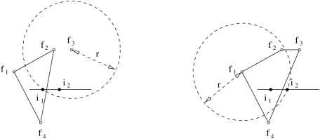
Figure 3: (Left) Point $i_{1}\in I$ is the leftmost intersection point between $\overline{p_{l}p_{r}}$ and the circle $C(f_{3},r)$. The segment $s_{1}=(p_{l},i_{1})$ is 1-well illuminated by the set $\mathcal{F}(s_{1})=\{f_{1},f_{2},f_{4}\}$. (Right) $\mathcal{F}(s_{2})=\mathcal{F}(s_{1})\cup\{f_{3}\}$. Point $i_{2}\in I$ is the rightmost intersection point between the circle $C(f_{1},r)$ and $\overline{p_{l}p_{r}}$. The segment $s_{2}=(i_{1},i_{2})$ is not 1-well illuminated since $i_{2}\not\in\mathrm{int}(\mathrm{CH}(\mathcal{F}(s_{2})))$.

Lemma 3.1

If two consecutive open segments $s_{k}$ and $s_{k+1}$ are $1$-well illuminated then $i_{k}\in I$ is also $1$-well illuminated.

Proof:

Suppose that $i_{k}\in I$ is not 1-well illuminated, this is, $i_{k}\notin(\mathrm{int}(\mathrm{CH}(\mathcal{F}(s_{k})))\cup\mathrm{int}(\mathrm{CH}(\mathcal{F}(s_{k+1}))))$. Since both open segments are 1-well illuminated, $i_{k}$ must lie on the boundary of both convex hulls. Since, by definition of $\mathcal{F}(s_{k})$, one of the two convex hulls is contained in the other, and both segments are inside the biggest one, $i_{k}$ is also contained. Hence, $i_{k}\in I$ is 1-well illuminated.

$\square$

Lemma 3.2

The open segment $s_{k}$ is $1$-well illuminated if $i_{k}$ and $i_{k-1}$ are both inside $\mathrm{CH}(\mathcal{F}(s_{k}))$.

Proof: By definition of $\mathcal{F}(s_{k})$, the segment $s_{k}$ is 1-well illuminated if it is interior to the convex hull of this set. Since this convex hull is obviously convex, the segment $s_{k}$ is 1-well illuminated when its endpoints are in the convex hull of $\mathcal{F}(s_{k})$. $\square$

Theorem 3.3

If the endpoints of $s$ as well as all $s_{k}$, with $k\in\{1,\dots,m\}$, are $1$-well illuminated, then $s$ is $1$-well illuminated.

Proof: Follows from Lemmas 3.1 and 3.2. $\square$

An efficient algorithm to solve the Decision Problem is then the following: Check if $i_{0}$ and $i_{m}$ are 1-well illuminated using the MER-Point algorithm. For all $k\in[1,\dots,m]$ we compute $CH(\mathcal{F}(s_{k}))$ by simply adding or deleting a point to $CH(\mathcal{F}(s_{k-1}))$ and check whether $s_{k}$ is 1-well illuminated. If all checks are true, then $s$ is 1-well illuminated; otherwise, it is not.

Proposition 3.1

Given a real number $r>0$, a set $F$ of $n$ light sources with limited illumination range $r$ and a line segment $s$, the algorithm described above decides if $s$ is $1$-well illuminated by $F$ in $\mathcal{O}(n\log n)$ time.

Proof: Let $F$, be a set of $n$ light sources with a limited illumination range $r$. Checking if $p_{l}$ and $p_{r}$ are $1$-well illuminated is linear using the MER-Point algorithm. Sorting the points in $I$ according to their $x$-coordinate takes $\mathcal{O}(n\log n)$ time. Computing the set of light sources that illuminate $p_{l}$ is linear but constructing its convex hull takes $\mathcal{O}(n\log n)$ time. Updating dynamically the convex hull every time we need to add or remove a light source can also be done in $\mathcal{O}(\log n)$ (amortized) time [5], and checking if both $i_{k-1},i_{k}$ are in the CH($\mathcal{F}(s_{k})$) takes $\mathcal{O}(\log n)$ time. Since we have at most $2n$ intersection points and we spend $\mathcal{O}(\log n)$ time on each one, this algorithm decides if $s$ is $1$-well illuminated by $F$ with range $r$ in $\mathcal{O}(n\log n)$ time. $\square$

Note that this procedure still works when each light source has a different range. Instead of having $n$ circles with the same radius, we have $n$ circles with different radii. After computing the intersection points between the $n$ circles and the line segment, the remaining procedure is exactly the same.

The Algorithm

We have an algorithm to decide if, given a range value, a line segment is 1-well illuminated. In order to compute the minimum range needed to 1-well illuminate the segment, we will apply the Parametric Search technique due to Megiddo [10, 11].

Let $F$ be a set of $n$ light sources.

Let $g$ be a monotonic function ($g(x)\geq g(y)$ if $x>y$) with a root. We want to convert our problem in a monotonic root-finding problem since we have an efficient decision algorithm to solve it. Now we define the function $g$ as follows:

$$g(\theta)=\left\{\begin{array}[]{ll}0,&\textrm{$s$ is \mbox{1-well} illuminated by $F$ with range $r=\frac{1}{\theta}$}\\ 1,&\textrm{$s$ is not \mbox{1-well} illuminated by $F$ with range $r=\frac{1}{\theta}$}\\ \end{array}\right.$$

We know how to compute if $s$ is 1-well illuminated using the decision algorithm just presented. Our goal to find the greatest root $\theta^{*}=\max\{\theta:g(\theta)=0\}$ using the Parametric Search and once we have it, the MER of $s$ is $r_{m}=\frac{1}{\theta^{*}}$.

Since we solve the decision problem in $O(n\log n)$ time, we can find this root in $O(n^{2}\log^{2}n)$ time. An small improvement in performance can be achieved using the following parallel decision algorithm. First, we lexicography sort all the light sources using $O(n)$ processors which takes $\mathcal{O}(\log n)$ time. We give each processor one light source so they compute all intersection points in constant time. Each processor has, at most, two intersections and has to check if they are inside the convex hull of the light sources illuminating them. Since the set of light sources is lexicography sorted, computing the needed convex hull takes $\mathcal{O}(\log n)$ time with the help of $\mathcal{O}(\frac{n}{\log n})$ additional processors. Performing the checks takes $\mathcal{O}(\log n)$ time. With a total number of $\mathcal{O}(\frac{n^{2}}{\log n})$ processors, we can decide if $s$ is $1$-well illuminated in $\mathcal{O}(\log n)$ time.

Proposition 3.2

Given a set $F$ of $n$ light sources in the plane and a line segment $s$, the Parametric Search computes the $\mathrm{MER}$ of $s$ in $\mathcal{O}(n^{2})$ time.

Proof: The sequential decision algorithm takes $S(n)\in\mathcal{O}(n\log n)$ time while the one running in parallel requires $T(n)\in\mathcal{O}(\log n)$ time when using $P(n)\in\mathcal{O}(\frac{n^{2}}{\log n})$ processors. So the total time to evaluate the function $g(\theta)$ and finding its greatest root using the Parametric Search, as well as computing the MER of $s$, is $\mathcal{O}(S(n)T(n)\log P(n)+T(n)P(n))\in\mathcal{O}(n\log n\times\log n\times\log(\frac{n^{2}}{\log n})+\log n\times\frac{n^{2}}{\log n})\in\mathcal{O}(n^{2})$ time. $\square$

4 The E-Voronoi Diagram Restricted to a Line Segment

In the previous section we have computed the minimum illumination range that a set of light sources must have in order to embrace all the points of a line segment. Now we go further and compute the closest embracing site for every point of the line segment which is equivalent to solve the problem of constructing the E-Voronoi diagram [3] restricted to a line segment $s=\overline{p_{l}p_{r}}$. With this structure, it is possible to make a query in $\mathcal{O}(\log n)$ time to know the minimum illumination range needed to embrace a point of $s$. As in the previous section, we will assume that $s$ is an horizontal line segment and that $p_{l}$ and $p_{r}$ are respectively the leftmost and rightmost points of $s$. The next definition can be found under the previous name of MIR-Voronoi region (MIR-VR) [3].

Definition 4.1

Let $F$ be a set of $n$ light sources in the plane. For every light source $f\in F$, the E-Voronoi region of $f$ with respect to the set $F$ is the set

$$\mathrm{E}\textrm{-}\mathrm{VR}(f,F)=\{x\in\mathbb{R}^{2}:f\in F\textrm{ is the closest embracing site for }x\}.$$

The set of all the E-Voronoi regions is called the E-Voronoi diagram of $F$ (formerly known as the MIR Voronoi Diagram [3]). An algorithm to compute the E-Voronoi diagram of $F$ restricted to a segment $s$ follows.

For each light source $f\in F$, we perform a sweep searching for the points of $s$ that belong to the $\mathrm{E}\textrm{-}\mathrm{VR}(f,F)$. When the sweeping for $f$ is done, we have computed all the components of the $\mathrm{E}\textrm{-}\mathrm{VR}(f,F)$ restricted to $s$ (note that the E-Voronoi region of a light source is not always connected [3]). When the sweeping is done for all the light sources of $F$, we have computed the E-Voronoi diagram of $F$ restricted to $s$.

Let us start computing the E-Voronoi region of a light source $f\in F$ restricted to $s$. Let $p_{f}$ be the closest point on $s$ to the source $f$. We will sweep from left to right (from $p_{f}$ to $p_{r}$) and then from right to left (from $p_{f}$ to $p_{l}$). When we are moving along $s$, we change from one E-Voronoi region to another when the point has two closest embracing sites or the point reaches the border of the convex hull of its current closest embracing set. In the first case, this corresponds to the intersection between $s$ and the perpendicular bisectors between the two closest embracing sites of the point. For that reason, we compute the intersection points between $s$ and the perpendicular bisectors between the light sources in $F\backslash\{f\}$ and $f$. We keep these intersection points as well as $p_{l},p_{f}$ and $p_{r}$ sorted by the $x$-coordinate in two lists (one for each type of sweeping), $L_{1}=\{p_{f},\ldots,p_{r}\}$ and $L_{2}=\{p_{f},\ldots,p_{l}\}$. The intersection points between $s$ and the convex hull of the closest embracing set of a point will be added to this list during the sweeping. As the $\mathrm{E}\textrm{-}\mathrm{VR}(f,F)$ may not be connected, while sweeping $s$ we might cross several of its components. So to catch up where each component starts or ends, we say that $p_{i}\in s$ is a starting (ending) point of the $\mathrm{E}\textrm{-}\mathrm{VR}(f,F)$ if it is the point where a component of the $\mathrm{E}\textrm{-}\mathrm{VR}(f,F)$ starts (ends). We will only explain the sweeping from left to right using the list $L_{1}$ (the sweeping from right to left is a mirror of this one).

For each $p_{i}\in L_{1}$ starting on $p_{i}=p_{f}$, we compute the convex hull of all light sources inside the circle with radius $d(f,p_{i})$. We use $H(f,p_{i})$ for this hull. Note that $f$ is on its boundary and call $H^{*}(f,p_{i})$ the obtained convex hull when deleting $f$ (the two edges adjacent to $f$ are called support lines). We will look for the points $p_{i}\in s$ such that $p_{i}\in\mathrm{int}(H(f,p_{i}))$ but $p_{i}\notin\mathrm{int}(H^{*}(f,p_{i}))$, this is, the points $p_{i}\in s$ such that $f$ is their closest embracing site. The following lemmas give the clues to the discretization of the sweeping.

Figure 4: Four possible situations for point $p_{i}$ concerning the location of $H^{*}(f,p_{i})$ represented by a dashed line and $H(f,p_{i})$ represented by a solid line. In cases (a) and (b), the segment between $p_{i}$ and $s_{i}$ is in $\mathrm{E}\textrm{-}\mathrm{VR}(f,F)$. In cases (c) and (d), $p_{i}$ is not in the E-Voronoi region of $f$ but $\mathrm{E}\textrm{-}\mathrm{VR}(f,F)$ starts after the point $s_{i}$ in both cases.

Lemma 4.1

Given a point $p_{i}\in L_{1}$ and the light source $f\in F$, let $p_{i}\in\mathrm{int}$ $(H^{*}(f,p_{i}))$. If $p_{i}\in\mathrm{E}\textrm{-}\mathrm{VR}(f,F)$ then $p_{i}$ is the ending point of a component of the $\mathrm{E}\textrm{-}\mathrm{VR}(f,F)$ restricted to $s$.

Proof: Given a point $p_{i}\in L_{1}$ and the light source $f\in F$, let $p_{i}\in\mathrm{int}(H^{*}(f,p_{i}))$. At first, $p_{i}\in\mathrm{int}(H^{*}(f,p_{i}))$ might suggest that $p_{i}\notin\mathrm{E}\textrm{-}\mathrm{VR}(f,F)$ but this may also suggest that we have just crossed a perpendicular bisector and now there is another light source in $F$ that also 1-well illuminates $p_{i}$. So if $p_{i}\in\mathrm{E}\textrm{-}\mathrm{VR}(f,F)$ then $p_{i}$ has two closest embracing sites. This means that the last points on the left of $p_{i}$ are also in the same component of the $\mathrm{E}\textrm{-}\mathrm{VR}(f,F)$ as $p_{i}$, but the points on its right are in a component of another E-Voronoi region. So $p_{i}$ is the ending point of a component of the $\mathrm{E}\textrm{-}\mathrm{VR}(f,F)$ restricted to $s$. $\square$

Lemma 4.2

Given two consecutive points $p_{i},p_{i+1}\in L_{1}$ and the light source $f\in F$, let $p_{i}\in\mathrm{int}(H(f,p_{i}))$ but $p_{i}\notin\mathrm{int}(H^{*}(f,p_{i}))$. If one of the support lines intersects $s$ between $p_{i}$ and $p_{i+1}$ on $s_{i}\in s$, then $[p_{i},s_{i})$ is a segment contained in the $\mathrm{E}\textrm{-}\mathrm{VR}(f,F)$ restricted to $s$.

Proof: Given two consecutive points $p_{i},p_{i+1}\in L_{1}$ and the light source $f\in F$, if $p_{i}\in\mathrm{int}(H(f,p_{i}))$ and $p_{i}\notin\mathrm{int}(H^{*}(f,p_{i}))$ then it is clear that the point is 1-well illuminated by $f$ so $p_{i}\in\mathrm{E}\textrm{-}\mathrm{VR}(f,F)$. We know that between $p_{i}$ and $p_{i+1}$ we do not cross any perpendicular bisector between $f$ and the other light sources in $F$ so if the $\mathrm{E}\textrm{-}\mathrm{VR}(f,F)$ ends before $p_{i+1}$, that is because the set $H(f,p_{i})$ is not an embracing set for all the points in the segment $\overline{p_{i}p_{i+1}}$. Let $s_{i}\in s$ be the intersection point between $s$ and one of the support lines, so the segment between $p_{i}$ and $s_{i}$ is 1-well illuminated by the set $H(f,p_{i})$ (see Figure 4(a)). On the other hand, $\overline{s_{i}p_{i+1}}\notin H(f,p_{i})$ so it is not 1-well illuminated by $f$. This means that $[p_{i},s_{i})$ is a segment contained in the E-Voronoi region of $f$ restricted to $s$. $\square$

Lemma 4.3

Given two consecutive points $p_{i},p_{i+1}\in L_{1}$ and the light source $f\in F$, let $p_{i}\in\mathrm{int}(H(f,p_{i}))$ but $p_{i}\notin\mathrm{int}(H^{*}(f,p_{i}))$. If $H^{*}(f,p_{i})$ intersects $s$ between $p_{i}$ and $p_{i+1}$, let $s_{i}\in s$ be the leftmost intersection point. Then $[p_{i},s_{i})$ is a segment contained in the $\mathrm{E}\textrm{-}\mathrm{VR}(f,F)$ restricted to $s$. Otherwise if $p_{i}$ is the leftmost intersection point between $H^{*}(f,p_{i})$ and $s$ then $p_{i}$ is the ending point of a component of the $\mathrm{E}\textrm{-}\mathrm{VR}(f,F)$ restricted to $s$.

Proof: Given two consecutive points $p_{i},p_{i+1}\in L_{1}$ and the light source $f\in F$, if $p_{i}\in\mathrm{int}(H(f,p_{i}))$ and $p_{i}\notin\mathrm{int}(H^{*}(f,p_{i}))$ then $p_{i}\in\mathrm{E}\textrm{-}\mathrm{VR}(f,F)$. If $H^{*}(f,p_{i})$ intersects $s$ between $p_{i}$ and $p_{i+1}$ then $H(f,p_{i})$ is not an embracing set for the whole segment $\overline{p_{i}p_{i+1}}$ (see Figure 4(b)). Let $s_{i}\in s$ be the leftmost intersection point between $s$ and the set $H^{*}(f,p_{i})$, only $[p_{i},s_{i})$ is a segment contained in the E-Voronoi region of $f$ restricted to $s$ because $\overline{s_{i}p_{i+1}}\in H^{*}(f,p_{i})$, so it is not 1-well illuminated by $f$. If $p_{i}$ is the leftmost intersection between $H^{*}(f,p_{i})$ and $s$ then $p_{i}$ is already the ending point of a component of the $\mathrm{E}\textrm{-}\mathrm{VR}(f,F)$ restricted to $s$. $\square$

Lemma 4.4

Given two consecutive points $p_{i},p_{i+1}\in L_{1}$ and the light source $f\in F$, let $p_{i}\notin\mathrm{int}(H(f,p_{i}))$ and $p_{i}\notin\mathrm{int}(H^{*}(f,p_{i}))$. If one of the support lines intersects $s$ between $p_{i}$ and $p_{i+1}$, let $s_{i}\in s$ be the leftmost intersection point. Then $s_{i}$ is the starting point of a component of the $\mathrm{E}\textrm{-}\mathrm{VR}(f,F)$ restricted to $s$. Otherwise if $p_{i}$ is the rightmost intersection point between the support lines and $s$ then $p_{i}$ is the ending point of a component of the $\mathrm{E}\textrm{-}\mathrm{VR}(f,F)$ restricted to $s$.

Proof: Given two consecutive points $p_{i},p_{i+1}\in L_{1}$ and the light source $f\in F$, if $p_{i}\notin\mathrm{int}(H(f,p_{i}))$ and $p_{i}\notin\mathrm{int}(H^{*}(f,p_{i}))$ then we know that $p_{i}\notin\mathrm{E}\textrm{-}\mathrm{VR}(f,F)$. Nevertheless, if one of the support lines intersects $s$ between $p_{i}$ and $p_{i+1}$ then there are points of $s$ between $p_{i}$ and $p_{i+1}$ whose embracing set is $H(f,p_{i})$, this is, these points belong to the E-Voronoi region of $f$. Let $s_{i}\in s$ be the leftmost intersection point between $s$ and the support lines (see Figures 4(c) and 4(d)). Point $s_{i}$ is on the border of $H(f,p_{i})$ which means that there will be interior points to the $H(f,p_{i})$ on $s$ after $s_{i}$. These points are 1-well illuminated by $f$ and $H(f,p_{i})$ is their embracing set so they belong to the E-Voronoi region of $f$. Thus the $\mathrm{E}\textrm{-}\mathrm{VR}(f,F)$ restricted to $s$ begins after the point $s_{i}\in s$. If $p_{i}$ is the rightmost intersection point between the support lines and $s$ then $\overline{p_{i}p_{i+1}}\notin\mathrm{int}(H(f,p_{i}))$ which means that $p_{i}$ is the ending point of a component of the $\mathrm{E}\textrm{-}\mathrm{VR}(f,F)$ restricted to $s$. $\square$

With these four lemmas, we are now able to sweep $s$ and know what to do every time we stop on $p_{i}\in L_{1}$. If $p_{i}$ is under the conditions of Lemma 4.2 or Lemma 4.3 and $p_{i}\neq s_{i}$, then $[p_{i},s_{i})$ is a segment contained in the E-Voronoi region of $f$ restricted to $s$. Point $p_{i}$ is probably a starting point of a component of the $\mathrm{E}\textrm{-}\mathrm{VR}(f,F)$ restricted to $s$ and we need to know if it is so we know the total extension of this component when we reach its ending point. The sweeping moves on to $s_{i}\in s$. If $p_{i}$ is under the conditions of Lemma 4.4 then the sweeping also moves on to $s_{i}\in s$. In the case that $p_{i}$ is itself an intersection point (as in the case of the lemmas 4.1, 4.3 and 4.4), the sweeping moves on to $p_{i+1}\in L_{1}$. If $p_{i}=p_{r}$ then we have reached the end of the list $L_{1}$ and we move to another sweep. It is clear that if $p_{r}\in\mathrm{E}\textrm{-}\mathrm{VR}(f,F)$ then $p_{r}$ is an ending point of a component of the $\mathrm{E}\textrm{-}\mathrm{VR}(f,F)$ restricted to $s$. When the sweeping is done for both lists, we repeat this procedure for another light source until we have them all studied.

Theorem 4.5

Let $s$ be a line segment and $F$ a set of $n$ light sources. The algorithm just described computes the E-Voronoi diagram of $F$ restricted to $s$ in $\mathcal{O}(n^{2}\log n)$ time.

Proof: Let $F$ be a set of $n$ light sources and $s$ a line segment. For each light source $f\in F$ we have to sweep $s$ stoping at the $\mathcal{O}(n)$ intersection points between $s$ and the perpendicular bisectors between $f$ and all the light sources in $F\backslash\{f\}$, as well as another intersection points computed during the sweeping. These intersection points have to be sorted which takes $\mathcal{O}(n\log n)$ time. Then we have to compute two convex hulls and this can also be done in $\mathcal{O}(n\log n)$ time. For each intersection point, we have to search for the cases that interest us in the lemmas 4.2, 4.3, 4.4 and 4.1, as well as update both convex hulls. Searching the intersections between $s$ and a convex hull or checking if a point is interior to a convex hull takes $\mathcal{O}(\log n)$ time. This is also the (amortized) time spent on dynamically updating the convex hull [5]. So the sweeping for each light source takes $\mathcal{O}(n\log n)$ time and it computes the restricted E-Voronoi region of the light source we are studying at the moment. Since we have $n$ light sources, the algorithm computes the E-Voronoi diagram of $F$ restricted to $s$ in $\mathcal{O}(n^{2}\log n)$ time. $\square$

Using this algorithm, we compute E-Voronoi diagram of $F$ restricted to $s$ and we can also compute the MER of $s$ using the following proposition. This technique takes $\mathcal{O}(n^{2}\log n)$ time but it is simpler than the one presented in the previous section.

Proposition 4.1

Let $s$ be a line segment and $F$ a set of $n$ light sources. The $\mathrm{MER}$ of $s$ is given by the biggest distance between a light source $f\in F$ and one of the extremes of its E-Voronoi region restricted to $s$.

Proof: Given a line segment $s$, the MER of $s$ is the biggest distance between a point of $s$ and its closest embracing site. By definition, a point is in the E-Voronoi region of $f\in F$ if $f$ is its closest embracing site. If we compute the biggest distance between a light source $f$ and a point of $s$ in its E-Voronoi region, we get the minimum illumination range needed to 1-well illuminate all the points in the $\mathrm{E}\textrm{-}\mathrm{VR}(f,F)$ restricted to $s$. Let $t$ be the intersection between $s$ and the $\mathrm{E}\textrm{-}\mathrm{VR}(f,F)$ and $p_{i}$ be an interior point of $t$. Assume that $p_{f}\in t$ (see Figure 5(a)), since $p_{f}$ is the closest point of $t$ to $f$, the distance between $p_{i}$ and $f$ increases when we are moving away from $p_{f}$ along $t$. So the minimum illumination range needed to 1-well illuminate $t$ is the biggest distance between one of its extreme points and $f$. Now suppose that $p_{f}\notin t$ (see Figure 5(b)), this means that the distance $d(f,p_{i})$ increases if we move $p_{i}$ towards one of the extremes of $t$ and decreases towards the other end. Again, the biggest distance between $f$ and a point of $t$ is the distance between one of its extremes and $f$. As each light source $f\in F$ has a minimum illumination range that can be computed by the distance between $f$ and one of the extremes of its E-Voronoi region restricted to $s$, the biggest of these minimum illumination ranges is the MER of $s$. $\square$

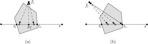
Figure 5: (a) The E-Voronoi region of $f\in F$ is the gray area, $d(f,t_{l})$ is the biggest distance between $f$ and a point of $t$, $d(f,p_{i})\leq d(f,t_{l}),p_{i}\in\overline{t_{l}t_{r}}$. (b) For a point $p_{i}\in\overline{t_{l}t_{r}}$, $d(f,p_{i})\leq d(f,t_{r})$ and the latter is the minimum illumination range needed to 1-well illuminate $t$.

The most interesting consequence of this algorithm is the following.

Theorem 4.6

Let $s$ be a line segment and $F$ a set of $n$ light sources. With a preprocess that can be done in $\mathcal{O}(n^{2}\log n)$ time, one can obtain the MER of a query point $q\in s$ in $\mathcal{O}(\log n)$ time.

Proof: Let $F$ be a set of $n$ light sources and $s$ a line segment. We can compute the E-Voronoi diagram of $F$ restricted to $s$ in $\mathcal{O}(n^{2}\log n)$ time using the algorithm described above. This preprocess allows us to have a structure that localizes a point $q\in s$ in $\mathcal{O}(\log n)$ time. Once the point is located, we know what is the E-Voronoi region that it belongs to, this is, we know what is the closest embracing site for $q$. The MER of $q$ is given by the distance between $q$ and its closest embracing site. $\square$

This algorithm and the one in the previous section are also useful when we want to compute the MER to 1-well illuminate a trajectory or a polygonal line. We can decompose the trajectory in several line segments and apply one of the algorithms to each part. This way, we compute a range for each piece and the greatest range of them all is the MER of the whole polygonal line or trajectory. An algorithm that shows how to compute all the different Closest Embracing Triangles for a line segment and their ranges can be found in [2].

5 Conclusions

The visibility problems solved in this paper consider $n$ light sources. We presented the linear algorithm MER-Point for computing a CET($p$) and its MER. This algorithm can also be used to decide if a point in the plane is 1-well illuminated. We also presented a quadratic algorithm to compute the MER of a line segment in the plane using the Parametric Search. Concerning the main subject in this paper, we presented another algorithm that computes the E-Voronoi diagram restricted to a line segment, as well as its MER. Both algorithms can also be extended to compute the MER of either open or closed polygonal lines.

References

- [1] M. Abellanas, S. Canales and G. Hern ndez: Buena iluminaci n. Actas de las IV Jornadas de Matem tica Discreta y Algor tmica (2004), 239–246.
- [2] M. Abellanas, A. Bajuelos, G. Hern ndez and I. Matos: Good Illumination with Limited Visibility. Proceedings of the International Conference of Numerical Analysis and Applied Mathematics 2005 (ICNAAM 2005), Wiley-VCH Verlag, 35–38.
- [3] M. Abellanas, A. Bajuelos, G. Hern ndez, I. Matos and B. Palop: Minimum Illumination Range Voronoi Diagrams. Proceedings of the 2nd International Symposium on Voronoi Diagrams in Science and Engineering (VD2005), 231–238.
- [4] M. Blum, R.W. Floyd, V. Pratt, R. Rivest and R. Tarjan: Time bounds for selection. Journal of Computer and System Sciences 7, (1973), 448–461.
- [5] G. Brodal and R. Jacob: Dynamic Planar Convex Hull. Proceedings of the 43rd Annual IEEE Symposium on Foundations of Computer Science (FOCS02), 617–626.
- [6] S. Canales: M todos heur sticos en problemas geom tricos, Visibilidad, iluminaci n y vigilancia. Ph.D. thesis, Universidad Polit cnica de Madrid (2004).
- [7] M.Y. Chan, D. Chen, F. Y.L. Chin and C. A. Wang: Construction of the Nearest Neighbor Embracing Graph of a Point Set. Journal of Combinatorial Optimization 11, no. 4, (2006), 435–443.
- [8] S. N. Chiu and I. S. Molchanov: A new graph related to the directions of nearest neighbours in a point process. Advances in Applied Probability 35, no. 1, (2003), 47–55.
- [9] A. Efrat, S. Har-Peled and J. S. B. Mitchell: Approximation Algorithms for Two Optimal Location Problems in Sensor Networks. Proceedings of the 14th Annual Fall Workshop on Computational Geometry, (MIT 2004).
- [10] N. Megiddo: Combinatorial Optimization with rational objective functions. Mathematics of Operations Research 4, (1979), 414 -424.
- [11] N. Megiddo: Applying parallel computation algorithms in the design of serial algorithms. Journal of the Association for Computing Machinery 30, no. 4, (1983), 852- 865.
- [12] N. Megiddo: Linear-time algorithms for linear programming in and related problems. SIAM Journal on Computing 12, no. 4, (1983), 759–776.
- [13] S. Ntafos: Watchman routes under limited visibility. Computational Geometry: Theory and Applications 1, no. 3, (Elsevier 1992), 149–170.
- [14] J. Smith and W. Evans: Triangle Guarding. Proceedings of the 15th Canadian Conference on Computational Geometry, (2003), 76–80.