A parent-centered radial layout algorithm for interactive graph visualization and animation

Abstract

We have developed (1) a graph visualization system that allows users to explore graphs by viewing them as a succession of spanning trees selected interactively, (2) a radial graph layout algorithm, and (3) an animation algorithm that generates meaningful visualizations and smooth transitions between graphs while minimizing edge crossings during transitions and in static layouts.

Our system is similar to the radial layout system of Yee et al. [26], but differs primarily in that each node is positioned on a coordinate system centered on its own parent rather than on a single coordinate system for all nodes. Our system is thus easy to define recursively and lends itself to parallelization. It also guarantees that layouts have many nice properties, such as: it guarantees certain edges never cross during an animation.

We compared the layouts and transitions produced by our algorithms to those produced by Yee et al. Results from several experiments indicate that our system produces fewer edge crossings during transitions between graph drawings, and that the transitions more often involve changes in local scaling rather than structure.

These findings suggest the system has promise as an interactive graph exploration tool in a variety of settings.

I.3.3Computer GraphicsPicture/Image GenerationViewing algorithms; H.5.0Information Interfaces and PresentationGeneral

1 Introduction

Visualization can help make graph structures comprehensible [7, 12, 23]. However, edge crossings can challenge human perception of relationships between nodes [8, 19, 24], yet graphs often come to us as tangled webs that cannot be depicted without crossings in a two-dimensional viewing plane.

Because trees can be laid out on a plane without edge crossings, a common approach is to base graph visualizations on spanning trees extracted from graphs [9, 15, 18, 26]. Although the resulting drawings may discard some potentially significant edge information, a clearer mental picture of the full graph may nonetheless result if users can easily and intuitively explore multiple layouts based on different spanning trees.

Yee et al. [26] describe a tool that draws radial tree layouts [3, 13, 22, 25] of breadth-first spanning trees, given a graph and a node selected to be the root (see Figure 1). A user may then select a new root node and the system transitions smoothly to a new layout based on the new root node. This transition is animated by a succession of linear interpolations of the polar coordinates of positions of each node in the old and new layouts. Thus, a user can interactively explore a graph that would otherwise be too complex to visualize or comprehend as a single, static drawing.

In drawings generated by Yee et al.’s radial layout method, successive generations of nodes lie on concentric circles centered on the root. Such layouts guarantee that all nodes of a given generation are equidistant from the root and lend themselves to a smooth animation process. However, symmetries in the tree can be obscured because distantly related nodes may be positioned close to each other in the final layout just because they belong to the same generation. And, during animations, numerous edge crossings may occur.

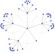
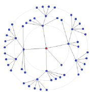
Figure 1: Two drawings for the same tree: Figure 1 is drawn by our layout algorithm, and Figure 1 is drawn by Yee et al.’s layout algorithm for Gnutellavision [26].

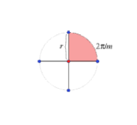
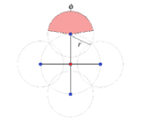
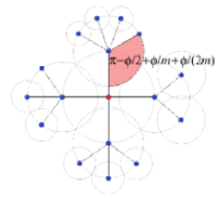
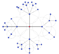
Figure 2: A visual overview of how our algorithm constructs a new layout for a graph. In Figure 2, the root is first placed at the center of the drawing surrounded by its children. Next, the root’s children are allocated containment arcs in Figure 2 where their descendants are positioned within Figure 2. The final static layout is shown in Figure 2.

Our approach is similar to Yee et al.’s in that it bases its drawings on breadth-first rooted spanning trees extracted from graphs, allows users to interactively change views of each graph by selecting a new root, and smoothly transitions between successive layouts by moving nodes along radial paths. However, unlike Yee et al., we place every subtree in the graph in a “parent-centric” circle surrounding its own subroot, instead of positioning each node on a “generation circle” centered on the root. This approach lends itself naturally to recursion, and naturally reflects the self-similar structure of recursively branching trees. Moreover, it guarantees that during the animation process the edges between parent and child never cross, a property Yee et al.’s algorithm does not provide. From an algorithmic perspective, each node’s position depends only on its parent and siblings, not on its entire generation. Because the dependencies in our layout are therefore very local, drawings and animations in our system are potentially computable in a single, parallelizable, traversal of the tree.

In broad strokes, our layout algorithm works as follows. First, we place the root in the center of the display with its children evenly distributed along a containment circle centered on the root. Second, we draw circles around the root’s children and evenly distribute their children along containment arcs that ensure that neither siblings nor cousins overlap. Then the second process just proceeds recursively, so that successively distant descendants of the root are positioned on successively smaller containment arcs (Figure 2).

Our layouts have several aesthetic virtues: They have a flowerlike, self-similar structure that differs from the “bulls-eye” appearance of Yee et al.’s layouts (compare Figure 1 and Figure 1). And even though the distance between root and nonroot nodes is less directly represented than in Yee et al.’s system, there are powerful visual cues to compensate: Within a lineage, edge lengths decrease monotonically with distance from root, and all siblings within a family are arrayed along visually salient arcs equidistant from their common parent. Also, our out-facing containment arcs ensure that the correlation between graph distance and Euclidean distance from the root is more reliable than in parent-centered approaches based on containment circles [13, 17, 22]. With regard to animating transitions, our algorithm ensures that sibling edges never cross when a new focal node is selected, and whenever the graph to be drawn is itself a tree.

2 Data Model and Algorithms

We assume that all graphs are connected, and regard any drawing of a spanning tree of a graph as a drawing of the graph. Since all edges are to be drawn as straight lines, we need only describe the mapping of nodes to points in the drawing plane (we use “node” to refer to both a vertex in a graph and to the location of the node on the drawing plane.) It is perhaps easiest to explain our algorithms in terms of a particular data model that completely describes a drawing in this restricted sense.

Rather than represent the position of all nodes of some graph in terms of a single polar coordinate system centered at the origin of the drawing plane that all nodes share, we only use the standard drawing-plane’s origin to represent the root node and its children. We represent every other node position in terms of polar coordinates centered at the node’s parent [10].

2.1 Parent-centered data model

We now formally define this concept. Given a tree $T$ and a drawing $D$ of $T$, we recursively define a parent-centered model of $(D,T)$ as follows. For any node $v$ of $T$, the polar coordinates of $v$ are given in the coordinate system

(basis 1, i.e., if $v$ is the root of $T$:)

sharing the origin with the drawing plane and zero degrees with the positive direction of the drawing plane’s $x$-axis,

(basis 2, i.e., if $v$ is a child of the root of $T$:)

having the root of $T$ as the origin and zero degrees as the ray from the root having the same direction as the positive direction of the drawing plane’s $x$-axis, or

(recursion, i.e., otherwise:)

having $v$’s parent in $T$ as the origin and the ray from $v$’s parent intersecting $v$’s grandparent as zero degrees.

Thus nodes having the same parent share the same coordinate system and nodes having different parents have different coordinate systems.

This data model applies to the static and dynamic layout algorithms described below. Note that we can (and do) represent any straight-line graph drawing this way, not just those produced by Algorithm 1 below.

2.2 Static layout algorithm

We define our static layout algorithm recursively as follows (see also Figure 2). When we say that a nonroot node lies on a containment circle, we are referring to the circle centered at the node’s parent that intersects the node. Note that if two siblings are the same distance from their parent (this is a property of the drawings Algorithm 1 produces) then they share the same containment circle.

Algorithm 1

Given a spanning tree $T$, for each node $v$ of $T$ let the coordinates of the root node be $(0,0)$ and for each nonleaf node $v$ let $v_{1},\ldots,v_{m}$ be $v$’s children. For each $i\in\{1,\ldots,m\}$ let the coordinates of $v_{i}$ (in the parent-centered model) be

(basis, i.e., if $v$ is the root:)

$(2\pi i/m,r)$, where $r$ is some user-defined value $>0$,

(recursion, i.e., otherwise:)

$(\pi-\phi/2+\phi i/m+\phi/(2m),r)$, where $\phi$ is some user-defined value $>0$ and $r$ is

• half of $v$’s magnitude, if $v$ has no siblings, otherwise

• the radius of the circle centered at $v$ that intersects the midway point between $v$ and $v$’s nearest sibling(s) on their shared containment circle.

Note that the value of $r$ for any nonroot node depends only on the node’s parent, so as claimed above all sibling nodes share the same value for $r$. This means they all lie on the same containment circle, which we call the containment circle of the parent node.

2.3 Animation algorithm

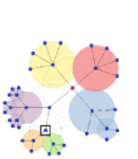
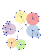
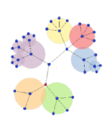
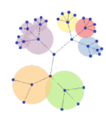
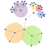
Figure 3: Isomorphic tree transition – Our visualization scheme transitions between two drawings of the same tree by scaling each parent node’s containment circle with its children. In this example, the user selects a new root node from the initial drawing in Figure 3. The containment circles highlighted during the transition in Figures 3 to 3 grow and shrink as the graph moves to the new drawing in Figure 3.

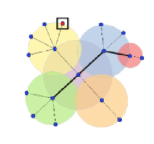
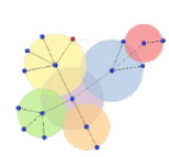
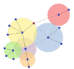
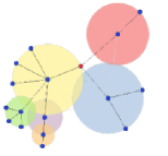
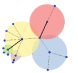
Figure 4: Spanning-tree-to-spanning-tree transition – The user’s selection of a new node invokes a new spanning-tree-based drawing. Edges that will fade out are highlighted in Figure 4; newly introduced edges are highlighted in Figure 4;

Our static layout algorithm leads to a simple and intuitive algorithm for animating transitions from one layout to another by interpolating between the parent-centered models of $D_{old}$ and a drawing produced by Algorithm 1 of a spanning tree of $G$ rooted at $v$, for any graph $G$, drawing $D_{old}$ and node $v$ of $G$ (see Figures 4 and 3).

Algorithm 2

1. Compute a breadth-first spanning tree $T$ of $G$ rooted at $v$.

2. Let $D_{new}$ be a drawing produced by running Algorithm 1 on $G$ and $T$.

3. Let $M_{old}$ be a parent-centered model of $(D_{old},T)$ and $M_{new}$ be a parent-centered model of $(D_{new},T)$

4. For each $t$ in an increasing sequence $0,t_{1},\ldots,t_{p},1$, output a polar drawing $D_{t}$ such that the model of $(D_{t},T)$ is described recursively as follows.

   (basis, i.e., if $v$ is the root of $T_{new}$):

   $(\theta,(1-t)r)$, where $(\theta,r)$ are the polar coordinates of $v$ in model of $M_{old}$.

   (recursion, i.e., otherwise:)

   $(t\theta_{new}+(1-t)\theta_{old},tr_{new}+(1-t)r_{old})$ otherwise, where, for $x\in\{old,new\}$, $(\theta_{x},r_{x})$ are the coordinates of $v$ in $M_{x}$.

Thus, the new root node moves in a straight line to the center of the new drawing, and each nonroot node moves via a finite approximation of a smooth interpolation between its parent-centered polar coordinates in the new and old drawings. In the resulting animation, newly-central families expand and fan out as they move toward the center, while newly-peripheral families shrink as they arc toward the periphery. Neighboring family circles are guaranteed not to interpenetrate. Note that any model $M_{t}=(D_{t},T)$ will not generally look like a model generated by Algorithm 1 since, for instance, the root of $T$ may not in $M_{t}$ lie on the origin of the drawing plane.

Our algorithm is built into a system that first displays a forced-directed layout [2] $D_{old}$ of a given graph $G$. A user then clicks on a node $v$ and the system runs Algorithm 2, the output of which, $D_{new}$, is set to $D_{old}$ the next time Algorithm 2 is called, which is the next time a user clicks on a node. Thus, $D_{old}$ is typically a drawing produced by Algorithm 1

(though it need not be).

There are different ways in which one can fix the times $t_{1},\ldots,t_{p}$ when generating the intermediate drawings of an animation. We adopted the slow-in, slow-out technique of Yee et al. in our implementation so that the values of $t_{1},\ldots,t_{p}$ are concentrated toward the boundary values $0$ and $1$.

2.4 Properties

Our algorithms have some noteworthy properties.

Aesthetics:

Our layout algorithm (1) ensures that all siblings are equally distant from their parent, (2) ensures that containment arcs of siblings and cousins do not overlap, and (3) produces layouts that provide clear indications (via edge-length and family shape) of closeness to the root.

Our animation process also guarantees that certain edges never cross. For any graph $G$, any drawing $D_{old}$ and a node $v$ of $G$, there is a choice for $\phi$ such that for any time $t\in[0,1]$, the edges corresponding to the spanning tree upon which $D_{t}$ is based do not cross in $D_{t}$. This has a number of consequences, including:

1. If $G$ is a tree then the drawing $D_{t}$ has no edge crossings.

2. For any node $v$ of $G$, the edges between $v$ and its children do not cross.

In the next section we describe experiments that test how well Algorithm 2 avoids edge crossings overall.

Parallelizability:

Note that all four steps of Algorithm 2 can be implemented as a single traversal of $T$ (i.e., during the breadth-first search that produces $T$). Algorithm 2 thus lends itself easily to parallelization, as a new process can be forked whenever a node of $T$ is traversed.

3 Experiments

Our experiments compare our algorithms’ layouts and animations to those produced by Yee et al.’s algorithms. In each experimental trial, a random graph was generated, two distinct root nodes within that graph were randomly selected, and the graph was then operated upon by both algorithms as they effected transitions from a spanning tree rooted at the first node to a spanning tree rooted at the second. Each experiment comprised 710 trials per algorithm, in which ten random graphs of order 30–100 (inclusive) were generated using the Erdös-Rényi model [4] with a 10% probability of an edge connecting any two nodes. In our first two experiments, we counted edge crossings during transitions by examining all edges present during the transition (whether derived from the new spanning tree or the old); a single crossing was counted during a trial if two edges crossed at any time during the transition, even if the edges crossed and uncrossed multiple times. In our last experiment, we measure the lengths of edges for sets of sibling nodes to their common parent in static layouts produced by the algorithms.

3.1 Isomorphic tree transitions

Because trees are by definition planar, transitional edge crossings are potentially avoidable in the special case where selection of a new root node does not change a tree’s edge set. In this experiment, we first extract a spanning tree from a graph rooted at a randomly selected root node and construct a new drawing. We then transition from this drawing to a second drawing of the same tree but with a different node selected as the focal point.

Figure 5 shows that our algorithms successfully produce zero crossings while Yee et al.’s algorithms produce many for this particular transition scenario. As illustrated in Figure 3, our approach avoids crossings because “family circles” simply expand or contract as they move without interpenetrating. In contrast, Yee et al.’s algorithms maintain visual continuity by preserving the direction of the edge from the new root node to its parent in the previous drawing. This can produce dramatically different drawings of the same tree, and result in crossings during the transitions.

This visual effect of our animations is similar to that of rigid-body animation methods [5, 6] as the user can mentally group subgraphs as separate objects and follow the movements more easily [16].

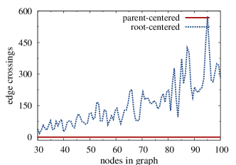
Figure 5: Isomorphic tree transitions
Our parent-centered visualization scheme produces no edge crossings when transitioning between drawings of the same tree, while Yee et al.’s root-centered system produces many.

3.2 Spanning-tree-to-spanning-tree transitions

In the second experiment, we counted edge crossings during transitions between two different spanning-tree-based drawings of the same graph. We first create a spanning-tree-based drawing for a graph rooted at a randomly selected node. We then select a second node for a new drawing based on a different spanning tree extracted from the graph. Unlike in the previous experiment, the edge sets of the two drawings are not the same in this experiment.

Our evaluation distinguishes “transient crossings involving fading-out edges” from “transient crossings involving final layout edges”. A crossing is transient but fading if at least one of the edges fades from the viewing plane during the animation sequence. A transient and non-fading crossing occurs when both edges are part of the final drawing.

As shown in Figure 6(a), the two visualization schemes produce a comparable number of transient but fading crossings. But Figure 6(b) shows that our algorithms produce fewer transient and non-fading crossings than Yee et al.’s, and that this difference grows with graph order.

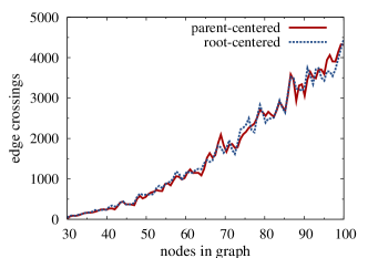
(a) Transient fading-out crossings

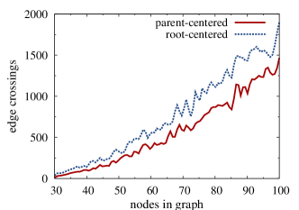
(b) Transient final layout crossings

Figure 6: Spanning-tree-to-spanning-tree transitions
The results in Figure 6(a) shows that both visualization schemes produce similar amounts of edge crossings during transitions between two different spanning-tree-based drawings. The results in Figure 6(a), however, clearly show that our parent-centered algorithms produced fewer crossings than Yee et al.’s root-centered algorithms.

3.3 Spanning tree sibling edge lengths

Since our approach positions nodes on containment arcs around their parent whereas Yee et al. positions nodes on concentric circles around the root node, the two systems produce different patterns of regularities. In this experiment we quantify those regularities.

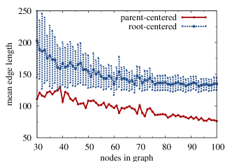
Figure 7: Spanning tree sibling edge lengths
Edge lengths from siblings to their common parent tend to decrease as graph size increases. In our algorithms, siblings are positioned equidistant to their common parent. In Yee et al.’s algorithms, edge lengths from siblings to common parent vary, as shown by standard deviations.

Figure 7 shows that as the generational distance increases from the root to nodes at a given depth in the tree, our system produces no variance among siblings in within-family distance from node to parent, whereas Yee et al.’s system produces substantial variance.

Conversely, in our system the distance from the root to nodes of a given generation can vary, whereas in Yee et al.’s system it does not. The variance arises in our case because our algorithm adjusts containment arcs to help prevent neighboring family circles from overlapping. Although this reduces the reliability of the length of edges as an indicator of distance from the root, the self-similar geometric pattern of family subsystems produces another cue that may well be more salient [14].

4 Discussion and Future Work

Behavioral tests will be needed to determine whether these alternative layout and transition algorithms are psychologically significant. But our statistical experiments indicate that the drawings and animated transitions generated by our algorithms conform to many established aesthetics for graph drawings [1, 19].

Taken in the context of the prior research on graph drawing aesthetics, these results suggest that our system should reduce a user’s mental effort and increase a user’s capacity to make reliable judgments and develop useful intuitions about complicated graph structures [8, 19, 24]. Our research thus lays the groundwork for future study of the layout and animation algorithms, of the psychological significance of our metrics, and of the functional validity of the graph aesthetics themselves.

With regard to our algorithms, two areas are particularly ripe for further study. First, the drawings produced by both ours and Yee et al.’s graph layout algorithm are not guaranteed to be planar; in our drawings, edge crossings can occur when long subtrees encroach on neighboring containment circles. An alternative method of allocating containment arcs might make it possible to guarantee planar drawings.

Second, with our approach, remote descendants of the root can become vanishingly small on the viewing plane. Our system does give users a natural solution to this problem: selecting a different root node so as to allocate more space to its descendants [20, 21]. However, future research could explore the algorithmic relation between our solution versus the distortion of the viewing plane in hyperbolic visualizations [11, 15]. There are clearly differences: we position and move siblings by constraining them to circles on a parent-centered Euclidean plane, whereas hyperbolic layout algorithms position and move siblings through a non-Euclidean space. The relative computational and psychological merit of these different approaches, however, remains to be determined.

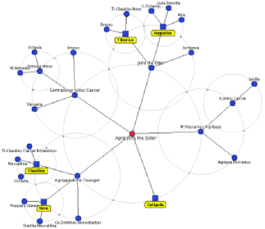
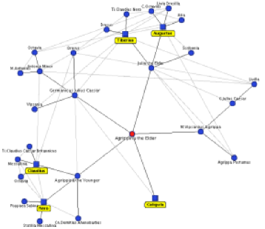
Figure 8: An example drawing of the Julio-Claudian Imperial family network generated by our layout algorithm. An edge between two entities in the graph denotes either a marital, parental, or adoption relationship. The Roman emperors in the graph are indicated by boxed labels. The graph is shown in Figure 8 with all the edges not included in the spanning tree in Figure 8 revealed.

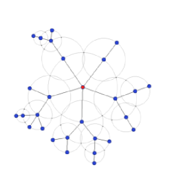
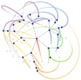
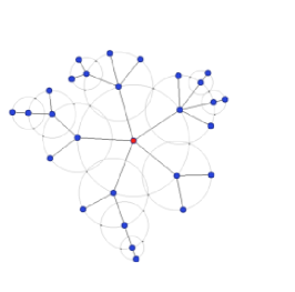
Figure 9: An example animation sequence generated by our animation algorithm. The user selects a new root node from an existing graph drawing in Figure 9 and the system transitions to the new layout in Figure 9. The trajectories of the nodes in the animation are highlighted in Figure 9.

5 Conclusion

We have presented a radial graph layout visualization scheme based on a parent-centered data model for spanning trees extracted from a graph. We introduced a static layout algorithm that produces drawings of graphs where the root’s children are evenly spaced on a circle centered at the root and the children of nonroot nodes are evenly spaced on a semicircle emanating from their parent. We also introduced an animation algorithm that smoothly transitions a graph from one spanning-tree-based layout to another. We conducted experiments to compare our experimental system with Yee et al.’s graph visualization system [26]. The results from these experiments suggest that our visualization and animation schemes could indeed help users understand and explore graphs.

References

- [1] Giuseppe Di Battista, Peter Eades, Roberto Tamassia, and Ioannis G. Tollis. Graph Drawing: Algorithms for the Visualization of Graphs. Prentice Hall, Upper Saddle River, New Jersey, 1999.
- [2] Peter Eades. A heuristic for graph drawing. Congressus Numerantium, 42:149–160, 1984.
- [3] Peter Eades. Drawing free trees. Bulletin of the Institute of Combinatorics and its Applications, 5:10–36, 1992.
- [4] P. Erdös and A. Rényi. On the evolution of random graphs. Publications of the Mathematical Institute of the Hungarian Academy of Sciences, 5:17–61, 1960.
- [5] Carsten Friedrich and Peter Eades. Graph drawing in motion. J. Graph Algorithms Appl., 6(3):353–370, 2002.
- [6] Carsten Friedrich and Michael E. Houle. Graph drawing in motion II. In GD ’01: Revised Papers from the 9th International Symposium on Graph Drawing, pages 220–231, London, UK, 2002. Springer-Verlag.
- [7] Herman, G. Melançon, and M. S. Marshall. Graph visualization and navigation in information visualization: A survey. IEEE Transactions on Visualization and Computer Graphics, 6(1):24–43, 2000.
- [8] Weidong Huang and Peter Eades. How people read graphs. In CRPIT ’45: proceedings of the 2005 Asia-Pacific symposium on Information visualisation, pages 51–58, Darlinghurst, Australia, Australia, 2005. Australian Computer Society, Inc.
- [9] T. J. Jankun-Kelly and Kwan-Liu Ma. Moiregraphs: Radial focus+context visualization and interaction for graphs with visual nodes. In Proceedings of the IEEE Symposium on Information Visualization, volume 00, pages 59–66, October 2003.
- [10] Matthias Kreuseler, Norma Lopez, and Heidrun Schumann. A scalable framework for information visualization. In INFOVIS ’00: Proceedings of the IEEE Symposium on Information Vizualization 2000, page 27, Washington, DC, USA, 2000. IEEE Computer Society.
- [11] John Lamping, Ramana Rao, and Peter Pirolli. A focus+context technique based on hyperbolic geometry for visualizing large hierarchies. In CHI ’95: Proceedings of the SIGCHI conference on Human factors in computing systems, pages 401–408, New York, NY, USA, 1995. ACM Press/Addison-Wesley Publishing Co.
- [12] Jill H. Larkin and Herbert A. Simon. Why a diagram is (sometimes) worth ten thousand words. Cognitive Science, 11(1):65–100, 1987.
- [13] Guy Melançon and Ivan Herman. Circular drawings of rooted trees. Technical report, Amsterdam, The Netherlands, 1998.
- [14] Daniel R. Montello, Sara Irina Fabrikant, Marco Ruocco, and Richard S. Middleton. Testing the first law of cognitive geography on point-display spatializations. In Werner Kuhn, Michael F. Worboys, and Sabine Timpf, editors, Spatial Information Theory. Foundations of Geographic Information Science, International Conference, COSIT Ittingen, Switzerland, September 24-28, 2003, Proceedings, volume 2825 of Lecture Notes in Computer Science, pages 316–331. Springer, 2003.
- [15] Tamara Munzner and Paul Burchard. Visualizing the structure of the World Wide Web in 3D hyperbolic space. In Proc. 1st Symp. The VRML Modelling Language: Special issue of Computer Graphics, pages 33–38. ACM Press, 14–15 1995.
- [16] Keith V. Nesbitt and Carsten Friedrich. Applying gestalt principles to animated visualizations of network data. In Sixth International Conference on Information Visualisation (IV’02), pages 737–743, 2002.
- [17] Quang Vinh Nguyen and Mao Lin Huang. A space-optimized tree visualization. In INFOVIS ’02: Proceedings of the IEEE Symposium on Information Visualization (InfoVis’02), page 85, Washington, DC, USA, 2002. IEEE Computer Society.
- [18] Steven Noel, Cheehung Henry Chu, and Vijay Raghavan. Visualization of document co-citation counts. In In Proceedings of the 2002 Intl. Conf. on Data Mining, pages 691–696, 2002.
- [19] Helen C. Purchase. The effects of graph layout. In OZCHI ’98: Proceedings of the Australasian Conference on Computer Human Interaction, page 80. IEEE Computer Society, 1998.
- [20] Manojit Sarkar and Marc H. Brown. Graphical fisheye views of graphs. In CHI ’92: Proceedings of the SIGCHI conference on Human factors in computing systems, pages 83–91, New York, NY, USA, 1992. ACM Press.
- [21] Doug Schaffer, Zhengping Zuo, Saul Greenberg, Lyn Bartram, John Dill, Shelli Dubs, and Mark Roseman. Navigating hierarchically clustered networks through fisheye and full-zoom methods. ACM Trans. Comput.-Hum. Interact., 3(2):162–188, 1996.
- [22] Soon Tee Teoh and Kwan-Liu Ma. Rings: A technique for visualizing large hierarchies. In GD ’02: Revised Papers from the 10th International Symposium on Graph Drawing, pages 268–275, London, UK, 2002. Springer-Verlag.
- [23] Edward Tufte. The Visual Display of Quantitative Information. Graphics Press, Cheshire CT, 1983.
- [24] Colin Ware, Helen Purchase, Linda Colpoys, and Matthew McGill. Cognitive measurements of graph aesthetics. Information Visualization, 1(2):103–110, 2002.
- [25] Graham J. Wills. Nicheworks — interactive visualization of very large graphs. Journal of Computational and Graphical Statistics, 8(2):190–212, 1999.
- [26] Ka-Ping Yee, Danyel Fisher, Rachna Dhamija, and Marti A. Hearst. Animated exploration of dynamic graphs with radial layout. In Proceedings of the IEEE Symposium on Information Visualization, pages 43–50, 2001.